1. Introduction
The dynamic of floating bodies is usually analyzed in the frequency domain using the linear diffraction–radiation method based on the boundary element methods (BEM). The problem is linearized supposing small displacements of the free surface and of the floating bodies. Several software programs have been developed to compute the solution of this problem such as HydroStar [
1], Nemoh [
2], Aqwa [
3], and Wamit [
4]. This first order theory enables for evaluating added mass and wave damping coefficients which are both parts of the radiation forces. The time–domain formulation of the dynamic equation, including those parameters, was introduced by Cummins [
5]. In this formulation, a convolution term appears which is computationally demanding when its evaluation is made by simple quadrature. This is why several models have been developed in order to approach this convolution term by a state–space model as in [
6] and [
7]. More exhaustive reviews of the different approaches used to replace the convolution term are proposed by Roessling et al. [
8], Unneland [
9], and Taghipour et al. [
10]. Pena-Sanchez proposes a comparison between some of these methods [
11]. Another advantage of using a state–space representation is to be able to use optimisation theory for state–space models such as Pontryagin’s maximum [
12]. This is especially useful for the control of Wave Energy Converters (WEC) [
13].
One of the most commonly used methods for replacing convolution by a state–space model is the Hankel Singular Value Decomposition method, introduced by Kung [
14]. This paper will focus on this method and the definition of the kernel function. A comparison will be made between the results in frequency and time domains.
This comparison will allow us to identify an omission in the definition interval of the kernel function. The relevancy of having, or not, a feedthrough term will be discussed. In order to understand the meaning of this feedthrough term, another approach will be tested. The approach will give a better understanding of having, or not, a feedthrough term with the HSVD method and also with other methods. This paper also exhibits the interest of extrapolating hydrodynamic coefficients.
It might be noticed that this paper does not seek to compare the HSVD method to other ones. The objective is to assess the influence of the definition interval of the kernel function on this method in order to establish whether other methods could also be affected.
2. Preliminaries
Before studying state–space formulations, a few prerequisites have to be reviewed. Some conditions must be respected to pass to the time–domain from the frequency-domain, and the point of this section to introduce those conditions. To be able to evaluate the accuracy of the different models from HSVD’s method, proposed in this paper, a basic case and calculation method is used. It has been chosen, for simplicity, to use a single cylinder for this test case. The diffraction–radiation calculation has been made using the HydroStar software [
1] with respect to the mesh constraint (the smaller facet’s diameter must be at least six times smaller than the smaller wavelength). The cylinder’s characteristics are given in
Table 1.
2.1. Frequency–Domain Formulation
The frequency Equation (
1) is established according to [
15]:
Using the complex notation, Equation (
1) becomes Equation (
2). In addition, solving Equation (
2), in the frequency domain, gives the reference RAO:
The reference RAO is given in Equation (
3):
With , the wave pulsation is between 0.01 and 3.0 rad by a step of 0.01 rad. For each pulsation, a wave from negative toward positive x-values is considered. The problem is then a 2D problem with only surge, heave, and pitch motions.
2.2. Time–Domain Formulation
The well-known Cummins’ equation implicitly uses the complex notation of
Section 2.1. The function
tends toward 0, and
tends toward
when
tends toward
∞; then, the following function is introduced:
Then, Equation (
1) becomes
The frequency domain equation can be stated in the time domain as shown in Equation (
6), which is the Cummins’ equation [
5].
where
Ogilvie [
15] has shown that the function
K can be computed using only the radiation damping coefficient. Considering as well that this function even leads to an equation that is widely used in the literature:
Assuming the causality of radiation and supposing that the system has no motion for
, Equation (
6) becomes
The added mass at infinite frequency,
, appears in Equation (
6) and an infinite integral appears in Equation (
8) requiring to know the asymptotic behavior of both added mass and damping.
2.3. Extrapolation of the Hydrodynamic Coefficients
As mentioned in
Section 2, there are constraints on the mesh for diffraction–radiation calculations. The maximum size of the mesh’s panels must be at least six times smaller than the minimum wave length. BEM methods consist of meshing boundaries only and building a full matrix equation, whereas CFD needs a mesh of the fluid volume and to build a narrow banded matrix equation. The BEM method usually remains much faster than CFD. However, the BEM computation at high frequencies requires a refined mesh and consequently a high rank matrix system which requires a lot of Random Access Memory. This is why the results of the calculation might be limited to a reasonable cut off frequency and asymptotically extrapolated in order to mitigate the computation time and memory requirements. It has been shown that it is possible to extrapolate radiation damping coefficient with a power law [
16]. By plotting the damping coefficient with a log scale, a linear behavior of the surge damping for high frequencies can clearly be seen in
Figure 1. In this case, the extrapolation was made up to a pulsation of 100
. The goal of the extrapolation is to avoid a truncation in the kernel function of Equation (
8). Indeed, since the integration is made on
, the extrapolation needs to be conducted until the damping coefficient tends toward zero and obtains a good estimation of the Fourier’s transform. The kernel function is the inverse Fourier’s transform of the radiation force terms.
To extrapolate the added mass, the Kramers–Kroening relations [
17] can be used or the Ogilvie relations [
15]. In practice, the Ogilvie’s relations are easier to manipulate because of the discontinuity in the Kramers–Kroening relations [
17]. The chosen relation is given in Equation (
10) for the cylinder which is a single solid MDOF system:
Figure 1 and
Figure 2 show the surge added mass and the wave damping with and without extrapolation. The extrapolation is also made to 100 rad
(
with D the diameter of the cylinder). The objective of extrapolating the added mass is to find the value of the infinite frequency added mass that will be useful for the different models presented in this paper. The infinite frequency added mass can also be directly computed by solving the equipotential free surface problem.
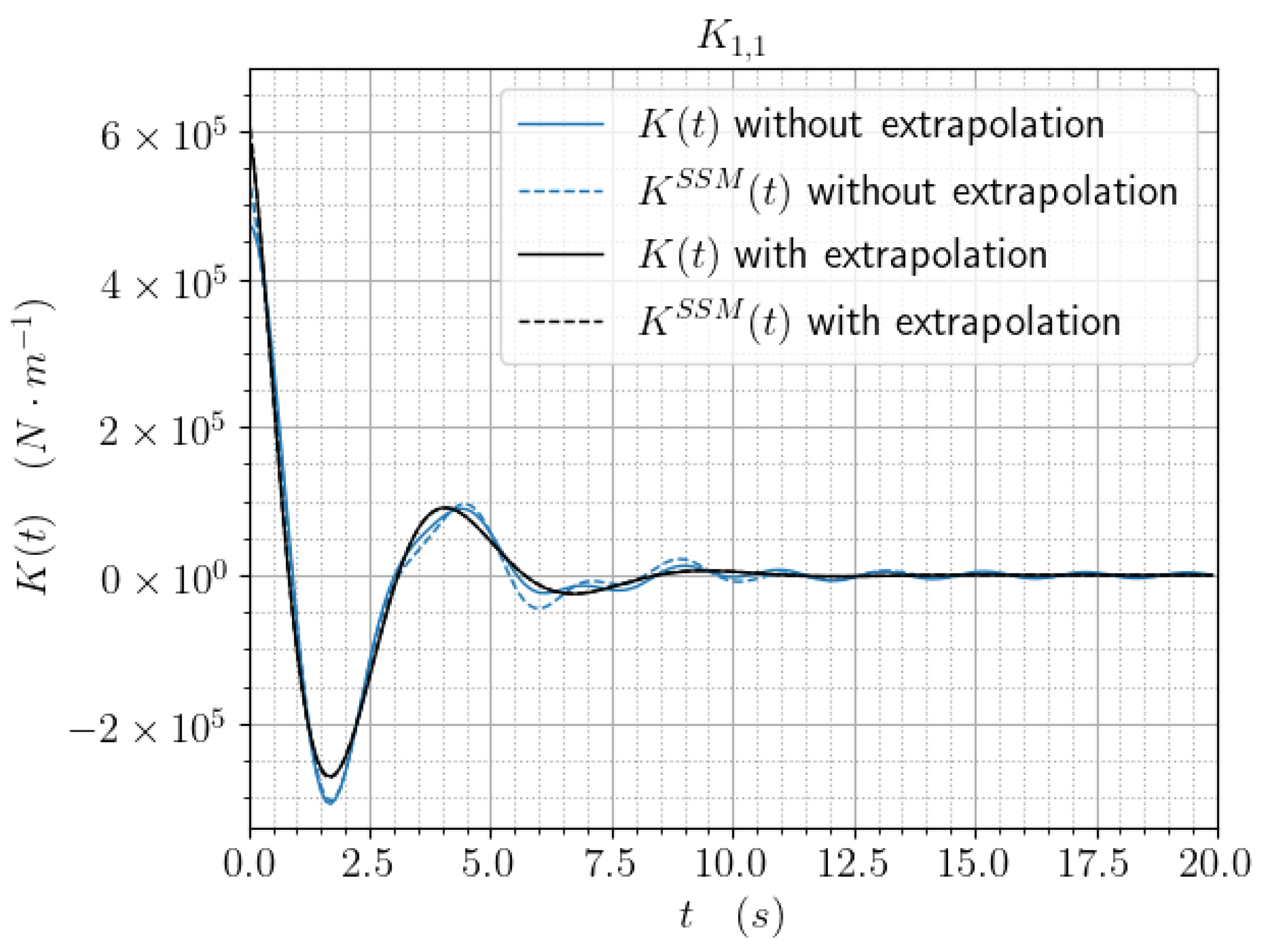
Figure 3 shows the kernel functions obtained with and without extrapolation of the hydrodyamic coefficients for surge motion on the first 20 seconds. A parasitic oscillation appears on the kernel function computed without extrapolation. The pulsation of this parasitic oscillation is the cut-off pulsation of the BEM computation. For this case, the cut off pulsation is 3 rad
. There are significant differences between the two kernel functions due to the loss of accuracy induced by the cut-off of the radiation damping.
Figure 1 shows that the radiation damping is around
at
rad
, which is far from the zero value that this expression is supposed to reach when
.
This section has introduced the bases needed for the presented study. It has also shown the importance of extrapolating the radiation damping to get an accurate evaluation of the kernel function.
The convolution term of Equation (
9) is not convenient for computation and for analysis. This is why it is often approached by a state–space model which is the object of the next section.
3. Classical Approach
This section first presents the formulation of the state–space model using the classical formulation of the kernel function. This formulation is discussed and completed in this section. The so-called classical approach refers to Equation (
8) that gathers both damping and added mass contributions into a single kernel function.
3.1. Formulation for a SDOF System
A way to approach the convolution term is to use the classical state–space representation used by Taghipour [
10] and Kristiansen [
18]. For a system with a single degree of freedom,
where
The expression of the output of the state–space model is given by the following equation:
where
,
,
and
. The order
N of the state–space model is the number of the most significant singular values.
One of the most commonly used algorithms to determine the matrix of the state–space model is the Hankel singular value decomposition (HSVD) introduced by Kung [
14]. A Python version of this algorithm has been developed by the NREL and can be found in the BEMIO package [
19]. A MATLAB version can also be found in WECSIM package [
19]. Perez [
20] details how to calculate the discrete state–space arrays from the Hankel matrix and then how to calculate the continuous state–space arrays using the discrete space state arrays by considering [
21].
In his method, Kung [
14] considers that there is no feedthrough matrix
. As a consequence, the kernel function from the state–space model is reduced to the expression of Equation (
14):
A more general formulation considering the feedthrough term, in the state–space formulation, is detailed by Perez [
20].
3.2. Formulation for a MDOF System (SSM1)
For a system with several degrees of freedom, the formulation is a little bit modified as presented in Equation (15). The state–space matrices are in Equation (15) tensors of the 4th order:
where
,
,
and
. State vector
and each subvector
. With the increase of the size of the model, it is desirable to decrease the order
N without losing accuracy. The data extrapolation of
Section 2.2 helps to apply the HSVD algorithm.
Figure 4 shows the kernel function and the kernel function from the state–space model (Equation (
14)), for
(i.e., only the four greatest singular values are kept to describe the kernel function) with and without extrapolation. It appears that the approximation is closer to the kernel function when extrapolation is used for hydrodynamic coefficients. As a consequence, extrapolating hydrodynamic coefficients lead to a reduction of the needed order of the state–space model.
For each pulsation, between
and
rad
by step of
rad
, a time–domain simulation is conducted, i.e., 300 monochromatic simulations are realized. A Runge–Kutta 4 algorithm (RK4) [
22] is used with a time step of
s on 30 periods. The amplitude of the time–domain response is then analyzed with an FFT algorithm and compared to the reference (Equation (
3)). The same conditions are used for every presented models. For reasons of simplicity, all the models presented in this paper are numbered in the order which they appear in the paper.
The time–domain response is polychromatic because of the transient effect even if the excitation force is monochromatic. Moreover, a ramp function is applied to the excitation force, on the first ten periods, to avoid strong transient flows at the earlier time steps of the simulation. Then, the time–domain response is polychromatic. This is why a convolution formulation is used for monochromatic waves. A similar process is used for experiments in wave tanks when a ramp is applied to the beginning of the wave maker motion.
Figure 5a,b compare this SSM1 model, for different orders of precision (number of singular values kept), to the reference model defined in
Section 2.1. The RAO obtained with the state–space model does not match the reference model RAO, especially for small pulsations and for pulsations around the peaks. After further investigations, it appears that the differences come from the definition of the kernel function
K.
3.3. Improved Formulation (SSM2)
Indeed, Equation (
8) is based on the Ogilvie relation [
15] assessing that
It is a very well-known fact [
23] that
The left term of Equation (
16) behaves differently in
. The function in the integral is reduced to the null function. Then, the left term is zero:
Thus, Equation (
16) becomes Equation (
19)
Writing the real part of Equation (
7), the kernel function can be expressed as follows:
By injecting Equation (
19) in Equation (
20), a partial re-definition of the kernel function appears:
The only difference is the values of
for
. Those values have no impact on
,
and
, but it is not the case of the feedthrough matrix
, which depends on
via the Tustin transform [
20]. It may also be noticed that the values of the integral in Equation (
8) are not changed if the values at
are changed. Moreover, computations deal with discrete time and using Equation (
21) will lead to inaccuracies in numerical integrations involving
, as, for example, Equation (
10). In that case, the definition of Equation (
8) is kept.
Figure 6a,b compare the SSM2 model with the correction of
, for different orders, to the reference model defined in
Section 2.1. The RAO obtained from the state–space model, with the correction of
, perfectly matches the reference model. The maximum error for surge RAO is 0.76 % at its peak (1.14 rad
) for order 20. The maximum error for pitch RAO is 0.78 % at its peak (1.14 rad
) for order 20.
3.4. State–Space Model without Feedthrough Term (SSM3)
Ref. [
24] shows some formulations of the state–space model which do not consider the feedthrough matrix
. For any state–space representation of any system, the feedthrough term is zero unless there is a direct path between the input and the output. Equation (
12) links the input and the output by a convolution term. Thus, it seems relevant to suppose that there is no direct path between the input
and the output
. Moreover,
involves that
is zero by application of the initial value theorem in the Laplace domain [
10,
20].
Then, a state–space model similar to the one proposed in [
24] is obtained. In this paper, another approach is used to determine the matrix of the state–space model using the companion matrix [
25]. A method using Prony’s series, proposed in [
26], also gives a state–space model without feedthrough matrix for a zero forward speed system:
It may be noticed that the improvement of the formulation of , considered in the previous paragraph, does not have any more effect since it only impacts the feedthrough matrix that has just been suppressed.
Figure 7a,b compare this simplified SSM3 model, for different orders, to the reference model defined in section
Section 2.1 The RAO obtained with the simplified state–space model does not perfectly match the reference model. The correspondence is quite good except for peaks. The maximum error for surge RAO is 5% at its peak (1.11 rad
) for order 20. The maximum error for pitch is also 5% at its peak (1.12 rad
) for order 20.
In this section, two different state–space models are tested considering or not the feedthrough matrix
. Two definitions of the kernel function have also been tried. It appears that the best model is the model SSM2 (
Section 3.3), which considers the feedthrough matrix with the improved definition of the kernel function proposed by this paper in Equation (
21).
3.5. Discussion on the Feedthrough Terms
As said in
Section 3.4, there is no reason to have a feedthrough term since there is no direct path between
and
. However,
Section 3.1 has shown that keeping the feedthrough matrix gives better results. This section will focus on the feedthrough matrix.
The classical model, developed in
Section 3.1, gives better results when keeping the feedthrough matrix
with respect to the improved definition of the kernel function (Equation (
21)). An aspect that has not been considered yet is the size of the time vector which is also the size of the discrete kernel function used by the HSVD algorithm. Let us introduce
which is the size of the time vector minus 1. Until now, the time vector’s values have gone from 0 to 100 seconds with
.
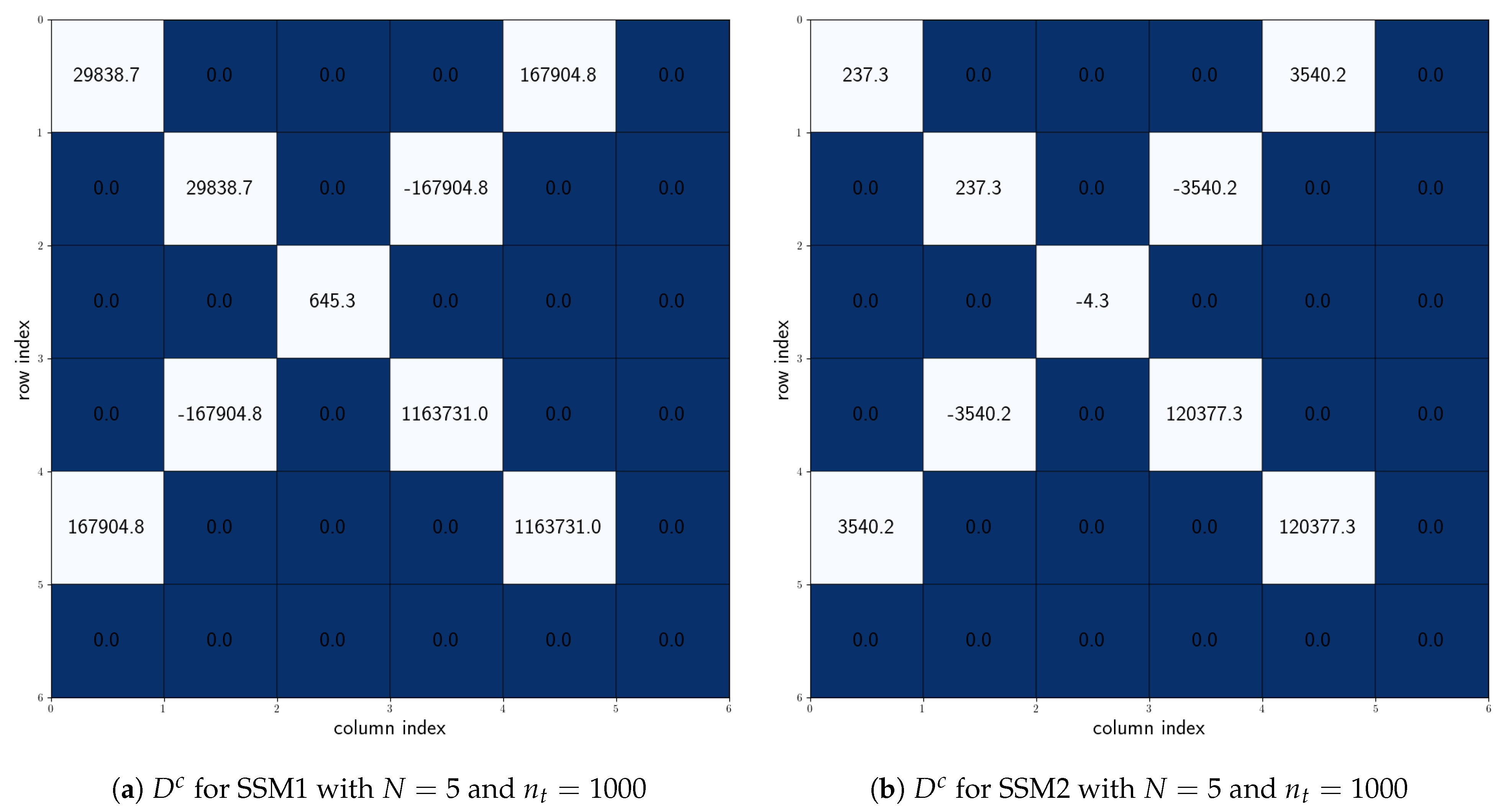
Figure 8 shows the evolution of non-zero values of
when
is increased. It appears that those values tend toward zero when
increases. Performing simulations with the new state–space matrices, for SSM1 and SSM3, gives a response that tends toward the reference RAO. Thus, the feedthrough matrix is a numerical artifact induced by an insufficient number of points in the time vector. Moreover, the accuracy of the other state–space arrays,
,
and
, is improved. Still, increasing the number of points is computationally demanding. Thus, even if it is not physically relevant, the feedthrough term should be kept to increase the accuracy, with a less costly computation, as in the case of a simple cylinder.
3.6. Comparison between SSM and Convolution for Irregular Waves
The RAO obtained with SSM1, SSM2, and SSM3 are the same as reference RAO if the time discretization is fine enough. In this section, the radiation forces obtained by convolution with the state–space radiation forces are compared. To do so, experimental data obtained on a vertical cylinder are used. The characteristics of this cylinder are given in
Table 2. The waves are generated using a Jonswap spectrum with a peak period of 1.9 s and a significant wave height of 10 cm. The natural periods in surge and pitch are close for the moored cylinder. The point is to compare the radiation forces, obtained with SSM and by convolution, for irregular waves knowing the motion in the time domain. The waves spread with an incidence of
so the movement is plan. The used motions, and the corresponding free surface elevation
, are plotted on
Figure 9. Speeds and accelerations are computed, from positions, using cubic splines [
27]. The sampling rate is 100 Hz.
The
jth component of the radiation force evaluated by convolution is given in Equation (29). In addition, the
jth component of the radiation force evaluated with the state–space model is given in Equation (
24). The convolution is computed keeping the experimental sampling rate (100 Hz):
Figure 10 shows the three components of the radiation force evaluated by convolution and with a state–space model. There are significants differences between both methods’ results. After further investigations, it appears that the differences are due to the definition of the kernel function
.
3.7. Kernel Function Definition Completion
As said in
Section 3.3, Equation (
16) is not true for every value of
t in
. Indeed, this relation must be adapted depending on the sign of
t. The case for
was treated in Equation (
19). Using the properties of sine and cosine functions, Equation (
19) can be expressed for any value of
t in
. The corresponding relation is given in Equation (
25):
Injecting Equation (
25) in Equation (
20) leads to the redefinition of the kernel function given in Equation (
26), which is the main original contribution of this paper:
Equation (
26) can be stated in a more compact form, Equation (
27), which underlines the discontinuity of the kernel function in
.
is the sign function:
Figure 11 shows the three components of the radiation force evaluated by convolution, with the new definition of the kernel function (Equation (
27)), and with a state–space model. It appears that the previous differences, seen in
Figure 10, have been corrected by using this new formulation of the kernel function. Indeed, since
, the upper integration limit of the convolution term becomes
t:
Moreover, the system is initially at rest, i.e.,
. Thus, the lower integration limit of the convolution term becomes zero:
Section 3.2 and
Section 3.3 have shown that the feedthrough matrix is not relevant, in terms of accuracy, if the discontinuity of the kernel function in
is not considered, which leads to differences between the obtained RAO and the reference RAO seen in
Figure 5. By correcting
, in
Section 3.3, those differences vanish. However, the feedthrough term is not physically relevant, which is why it has been deleted in
Section 3.4. Removing the term implies a loss of accuracy. To correct it, the time discretization must be refined, which involves a significant increase in computation time for the HSVD algorithm. In addition, since the best model (SSM2) is the one considering the discontinuity of the kernel function, it is legitimate to suspect this discontinuity to be responsible for the loss of accuracy for SSM3. In order to be sure, a new approach, considering continuous functions, will be proposed in this paper.
4. Other Approach
This section first presents the formulation of the state–space model using an original formulation of the kernel function split into two kernel functions. This formulation is validated and linked to the classical one in order to better understand the feedthrough term. In this section, another approach will be considered in order to avoid discontinuity as it is the case with the classical approach.
4.1. Time–Domain Formulation
The start point remains the same, i.e., Equation (
1), but the acceleration and speed terms of the radiation are not gathered, which leads to Equation (
30):
with the continuous kernel functions,
Thanks to Wehausen [
28], it appears relevant to derivate
. After having verified each assumption of the Leibniz integral rule, Ka can be derivated under the integral sign and the following expression appears:
Using the Ogilvie’s relation, Equation (
34) can be expressed
With
The integral of Equation (
37) is introduced
As in [
29], the function
(defined in Equation (
8)) can be approached by Equation (
38) using Prony’s series. Thus, it is also possible for
:
All the kernel functions oscillate around zero. This means that they have no continuous component. As a consequence,
can not have zero value. Then, it is possible to integrate:
Since
, Equation (
34) can be prolongated by continuity
It can be noticed that functions
and
are both symmetrical:
In practice, using Prony’s series, instead of numerical integration, gives more accurate results without having a small time-step, whereas numerical integration (trapeze or Simpson) needs a small time-step to have sufficient accuracy. The algorithm used to interpolate the kernel function with Prony’s series is detailed in [
30]. The Prony’s interpolation of
can also be used for extrapolation in
Section 2.2.
4.2. State–Space Model (SSM4)
Since the radiation force is separated in two parts, there are two state–space models. The first one is for the added mass radiation force and the second is for the damping radiation force:
Figure 12a,b compare this SSM4 model, for different orders, to the reference model defined in
Section 2.1. The RAO obtained with the two combined state–space models does not match the reference model RAO, especially for small pulsations and for pulsations around the peaks. It can be noticed that the gap between the RAO obtained and the reference RAO is half of the gap seen in
Figure 5a,b. Then, it is legitimate to suspect
, and
, to be responsible for those differences. However, in this case, the Kernel function does not take into account the simplification of the first model of
Section 3.2.
4.3. State–Space Model without Feedthrough Term (SSM5)
As it was done for the classical state–space model, where Equation (
22) was written without the feedthrough matrix, the two following systems are obtained:
Figure 13a,b compare this simplified SSM5 model, for different order, to the reference model defined in
Section 2.1. The RAO obtained with the two combined state–space models perfectly match the reference model RAO.
In this section, a model using continuous kernel functions has been presented. The model is actually the combination of two independent state–space models which are both giving a part of the radiation forces. For those two sub-models, the feedthrough arrays
and
are first considered. Then, a model without feedthrough is tried. It appears that the best model is the one where there are no feedthrough arrays, which is the model SSM5 (
Section 4.4).
4.4. Discussion on the Feedthrough Terms
The proposed model, developed in
Section 4, gives better results when deleting the feedthrough matrices
and
. However, in this case, the Kernel function does not take into account the simplification, of the first model of
Section 3.2, in the kernel functions, so a numerical issue can be suspected, as for the classical model.
Figure 14a,b show the evolution of non-zero values of
and
when
is increased. It appears that those values tend toward zero when
increases. Performing simulations with the new state–space matrices, for SSM4, gives a response that tends toward the reference RAO. Thus, the feedthrough matrices are numerical artifacts induced by an insufficient number of points in the time vector. However, contrary to the classical model, the accuracy of the other state–space matrices is not significantly improved since SSM5 is already close to the reference RAO. Thus, the feedthrough terms may be deleted, instead of increasing
, since it gives accurate results with a less costly computation for the HSVD algorithm.
4.5. Comparison between SSM and Convolution for Irregular Waves
As for
Section 3.6, the radiation force obtained by convolution and by state–space modeling will be compared. However, this time, upper integration limits of the convolution term can not be reduced a priori because
and
.
Figure 15 shows a perfect match between both evaluations. Moreover, the obtained results perfectly correspond to the results shown in
Figure 11. Indeed, the radiation force can be expressed by Equation (
46).
According to Equation (
32) and Equation (
34),
Thus, Equation (
46) can be developed to obtain Equation (
48):
For a zero speed system, Equation (
48) is reduced to Equation (
49):
Thus, the upper integration limit of the convolution term becomes t, even if and .
The size of the obtained model is twice as big as the size of the classical model. As a consequence, time domain simulations are more computationally demanding with this model than with the classical one. In the following paragraph, a solution is proposed to reduce this model size.
4.6. Model Reduction
The computation time, for time domain simulations, is directly impacted by the order of the model. Let
N be the order of the classical model. The approach of this section results in two sub-models of order
N, i.e., a model of order
. To reduce this model, the relations between
and
are used. The radiation force can be expressed, according to Equation (
49), as follows:
where
is the output of the state–space model. The
g function can then be introduced:
Which leads to
Equation (
53) is related to the corrected model of
Section 3.3. It might be noticed that the term
disappears If an analytical expression of Kernel function is considered. This is the case for the Prony’s series method [
26], for example, where the kernel function is expressed as a sum of analytical functions that ignore the discontinuity in
. However, since the area under a point is 0,
. However, this is not the case for methods working with a discrete kernel function such as the HSVD method. Indeed, the term
remains and depends on the time discretization. This is why a diminution, of the terms of feedthrough matrix, is observed in
Figure 8 when decreasing the time step.
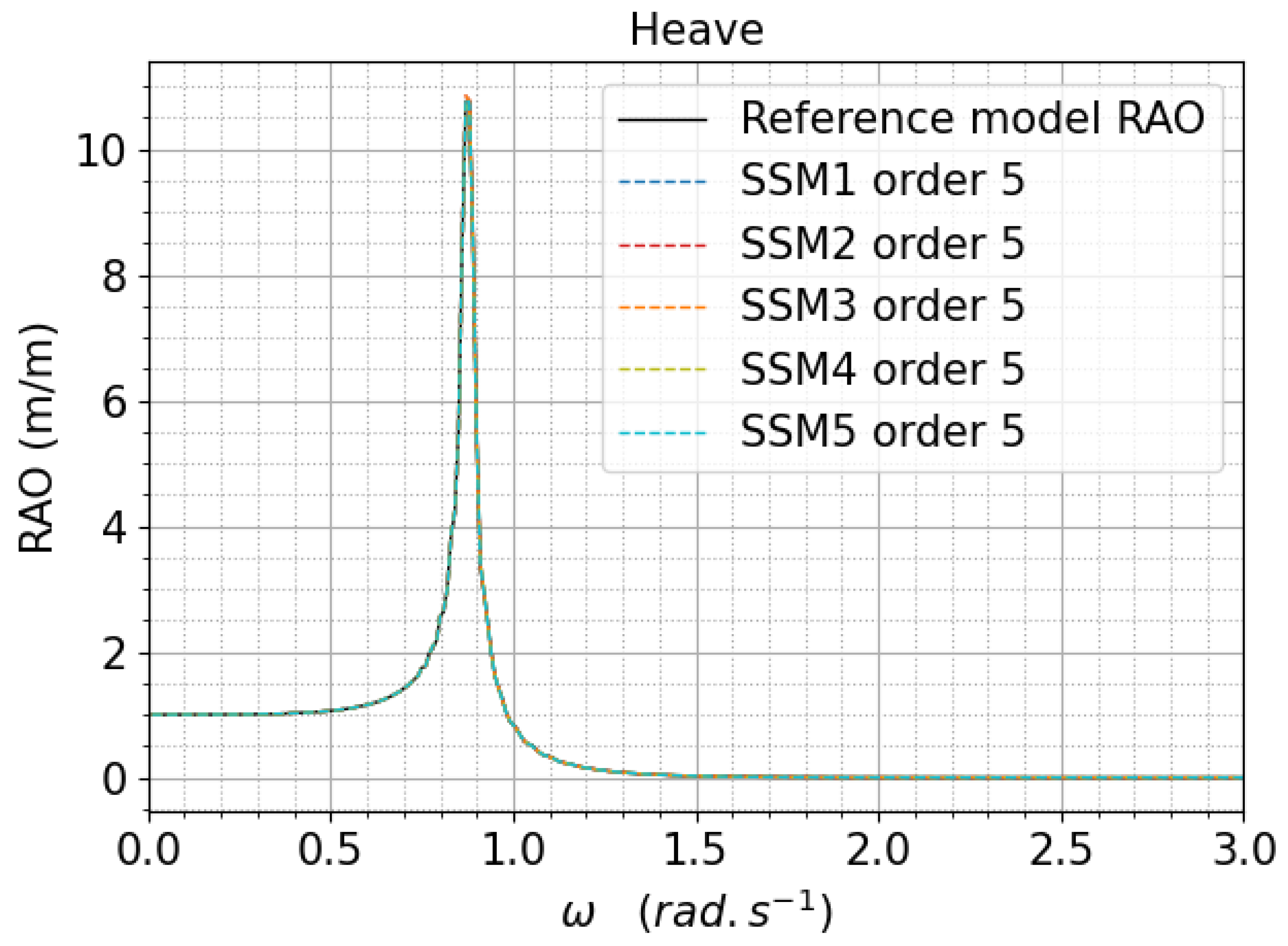
5. Heave Motion
This section deals with the heave motion that is not discussed in the previous sections because of its specific behavior. The heave motion has not been used in this paper because it does not depend on the state–space model’s formulation. The similarity between the reference RAO and the models, SSM1 to SSM5, can be seen in
Figure 16.
Figure 17 shows a significant decrease of the terms in the feedthrough when changing the definition of the kernel function from Equation (
8) to Equation (
21). The heave term is already relatively small with the first definition, so the impacts of the proposed improvement in heave motion are not significant. This fact is due to numerical values and is, a priori, specific to the studied device.
6. Conclusions
The results of diffraction radiation method are expressed in the frequency domain. The radiation force is decomposed into the added mass and the radiation damping, which are both frequency dependent. It is very common to gather the added mass and the radiation damping terms using the notation for complex numbers. At that point, the added mass and the damping can be stated into an equivalent damping. Olgivie’s relations are used to express the kernel function from this equivalent damping. Stating the kernel function in the time–domain requires knowing the asymptotic behavior of the radiation terms in the frequency-domain in order to avoid truncation issues. Indeed, cutting-off radiation damping, before it is close to zero, leads to inaccuracies in the kernel function. Moreover, it is more difficult to approach the kernel function, by a state–space model with a low order, without having converged hydrodynamic coefficients in the first place. Extrapolating radiation terms is a good compromise between computational demand and accuracy since it requires fewer resources than diffraction–radiation computations at high frequency. A comparison between frequency- and time–domain is used for 300 pulsations.
The comparison between the reference RAO and SSM1 shows significant differences. Deleting the feedthrough term, which is a numerical artifact, gives SSM3, which also differs from the reference RAO. Investigations on the definition of the kernel function have shown an omission in its definition interval. Considering a full interval formulation gives SSM2, which perfectly matches the reference RAO. Another way to improve the accuracy of the result is to decrease the time step for SSM3, but this method dramatically increases the computation time of the SVD algorithm. A completed formulation of the kernel function is proposed in this paper and shows two things. First, its causality () does not have to be assumed since it is an intrinsic property of radiation, valid for any device. The second point is the discontinuity in , and this discontinuity leads SSM2 to give better results than other formulations.
Another approach is tried in order to get a better understanding of the the role of the feedthrough term. Without gathering both radiation terms, the time–domain equation has two convolution terms and thus two state–space models. The kernel functions of those convolutions terms are continuous. In addition, contrary to the classical formulation, the feedthrough matrices are simply numerical artifacts to remove.
By linking this other approach to the classical one, it appears that the feedthrough matrix contains the discontinuity of the discrete kernel function. As a consequence, the omission of this discontinuity when stating methods based on a discrete time–domain kernel function, such as HSVD, will lead to a mismatch between frequency- and time–domain results. A computationally demanding solution is to decrease the time step in order to extinguish the term
in Equation (
53). Another solution is to keep the feedthrough term, even if it has no physical meaning, since it informs the state–space model of the discontinuity of the kernel function.
The used cylinder geometry, used in this paper, is very simple and particular. As a consequence, some results are specific to this geometry. The fact that heave motion is not affected by
is, a priori, specific to this geometry. Moreover, the extrapolation of radiation damping will not be so easy for all geometries. The power law, used in
Section 4, will not be relevant for complex geometries. For complex geometries, a different method should be used to extrapolate if possible. Otherwise, computationally demanding calculations will be necessary.
Author Contributions
Conceptualization, R.L.-L.B.; methodology, R.L.-L.B. and M.L.B.; software, R.L.-L.B.; validation, R.L.-L.B., M.L.B., J.-F.C., and M.B.; formal analysis, R.L.-L.B., M.L.B., J.-F.C., and M.B.; investigation, R.L.-L.B.; writing—original draft preparation, R.L.-L.B.; writing—review and editing, R.L.-L.B., M.L.B., J.-F.C., and M.B. All authors have read and agreed to the published version of the manuscript.
Funding
The authors acknowledge the Ph.D. scholarship from Région Bretagne and IFREMER.
Institutional Review Board Statement
Not applicable.
Informed Consent Statement
Not applicable.
Data Availability Statement
Available upon request from the authors.
Acknowledgments
Not applicable.
Conflicts of Interest
The authors declare no conflict of interest.
Nomenclature
| i | unit imaginary number |
| n | number of solids |
| N | order of the state–space model |
| mass matrix |
| added mass |
| infinite frequency added mass |
| radiation damping |
| generalized motion vector in the frequency domain |
| generalized speed vector in the frequency domain |
| generalized acceleration vector in the frequency domain |
| generalized motion vector in the time domain |
| generalized speed vector in the time domain |
| generalized acceleration vector in the time domain |
| state matrix (classical model) |
| input matrix (classical model) |
| output matrix (classical model) |
| feedthrough matrix (classical model) |
| state vector (classical model) |
| state–space output (classical model) |
| kernel function in time domain |
| stiffness matrix |
| incident wave excitation force in the frequency domain |
| incident wave excitation force in the time domain |
| radiation forces in the time domain |
| external forces in the time domain |
| added mass kernel function in time domain |
| radiation damping kernel function in time domain |
| state–space output (other approach) |
| state matrix (other approach) |
| input matrix (other approach) |
| output matrix (other approach) |
| feedthrough matrix (other approach) |
| state vectors (other approach) |
| p, j, k | arrays’ indices |
| t | time |
| pulsation |
| wave length |
| D | cylinder diameter |
| HSVD | Hankel Singular Value Decomposition |
| RAO | Response Amplitude Operator |
| BEM | Boundary Element Method |
| CFD | Computational Fluid Dynamics |
| SSM | state–space model |
| SDOF | Single-Degree-Of-Freedom |
| MDOF | Multi-Degree-Of-Freedom |
References
- Chen, X.B. Hydrodynamics in Offshore and Naval Applications—Part I. In Proceedings of the 6th International Conference on HydroDynamics, The University of Western Australia, Perth, Australia, 24–26 November 2004; p. 28. [Google Scholar]
- Fàbregas Flavià, F.; McNatt, C.; Rongère, F.; Babarit, A.; Clément, A. A numerical tool for the frequency domain simulation of large arrays of identical floating bodies in waves. Ocean. Eng. 2018, 148, 299–311. [Google Scholar] [CrossRef] [Green Version]
- Gourlay, T.; von Graefe, A.; Shigunov, V.; Lataire, E. Comparison of AQWA, GL Rankine, MOSES, OCTOPUS, PDStrip and WAMIT With Model Test Results for Cargo Ship Wave-Induced Motions in Shallow Water. In Proceedings of the ASME 2015 34th International Conference on Ocean, Offshore and Arctic Engineering, St. John’s, NL, Canada, 31 May 2015; American Society of Mechanical Engineers: New York, NY, USA; p. V011T12A006. [Google Scholar] [CrossRef] [Green Version]
- Newman, J.; Sclavounos, P.D. The computation of wave loads on large offshore structures. In Proceedings of the “Boss” Conference, Trondheim, Norway, 1988; pp. 1–18. Available online: http://classify.oclc.org/classify2/ClassifyDemo?wi=19291010 (accessed on 13 July 2021).
- Cummins, W.E. The Impulse Response Function and Ship Motions; Technical Report 1661; David Taylor Model Basin: Washington, DC, USA, 1962. [Google Scholar]
- Yu, Z.; Falnes, J. State-space modelling of dynamic systems in ocean engineering. J. Hydrodyn. 1998, 10, 1–17. [Google Scholar]
- Faedo, N.; Peña-Sanchez, Y.; Ringwood, J.V. Moment-Matching-Based Identification of Wave Energy Converters: The ISWEC Device. IFAC-PapersOnLine 2018, 51, 189–194. [Google Scholar] [CrossRef]
- Roessling, A.; Ringwood, J. Finite order approximations to radiation forces for wave energy applications. In Advances in Renewable Energies Offshore: Proceedings 1st International Conference on Renewable Energies Offshore; CRC Press: London, UK, 2014; Renew: 2014. [Google Scholar]
- Unneland, K. Identification and Order Reduction of Radiation Force Models of Marine Structures. Ph.D. Thesis, Norwegian University of Science and Technology, Trondheim, Norway, 2007. [Google Scholar]
- Taghipour, R.; Perez, T.; Moan, T. Hybrid frequency–time domain models for dynamic response analysis of marine structures. Ocean. Eng. 2008, 35, 685–705. [Google Scholar] [CrossRef]
- Pena-Sanchez, Y.; Faedo, N.; Ringwood, J.V. A Critical Comparison Between Parametric Approximation Methods for Radiation Forces in Wave Energy Systems. In Proceedings of the 29th International Ocean and Polar Engineering Conference, Honolulu, HI, USA, 25–30 June 2019; p. 9. [Google Scholar]
- Phogat, K.S.; Chatterjee, D.; Banavar, R.N. A discrete-time Pontryagin maximum principle on matrix Lie groups. Automatica 2018, 97, 376–391. [Google Scholar] [CrossRef] [Green Version]
- Faedo, N.; Olaya, S.; Ringwood, J.V. Optimal control, MPC and MPC-like algorithms for wave energy systems: An overview. IFAC J. Syst. Control. 2017, 1, 37–56. [Google Scholar] [CrossRef] [Green Version]
- Kung, S. A new identification and model reduction algorithm via singular value decompositions. In Proceedings of the 12th Asilomar Conference on Circuits, Systems and Computers, Pacific Grove, CA, USA, 6–8 November 1978; pp. 705–714, ISBN 9780780351486. [Google Scholar]
- Ogilvie, T. Recent progress toward the understanding and prediction of ship motions. In Proceedings of the The Fifth Symposium on Naval Hydrodynamics, Bergen, Norway, 10–12 September 1964; pp. 3–128. [Google Scholar]
- Bao, W.; Kinoshita, T. Asymptotic solution of wave-radiating damping at high frequency. Appl. Ocean. Res. 1992, 14, 165–173. [Google Scholar] [CrossRef]
- Bruzzoni, P.; Carranza, R.M.; Lacoste, J.R.C.; Crespo, E.A. Kramers/Kronig transforms calculation with a fast convolution algorithm. Electrochim. Acta 2002, 48, 341–347. [Google Scholar] [CrossRef]
- Kristiansen, E.; Hjulstad, S.; Egeland, O. State-space representation of radiation forces in time–domain vessel models. Ocean. Eng. 2005, 32, 2195–2216. [Google Scholar] [CrossRef]
- Wendt, F.; Yu, Y.H.; Nielsen, K.; Ruehl, K.; Bunnik, T.; Touzon, I.; Nam, B.W.; Kim, J.S.; Kim, K.H.; Janson, C.E.; et al. IEA OES Task 10 WEC Modelling Verification and Validation. In Proceedings of the 12th European Wave and Tidal Energy ConferencEuropean Wave and Tidal Energy Conference, Cork, Ireland, 27 August–1 September 2017; p. 8. [Google Scholar]
- Perez, T.; Fossen, T.I. Time- vs. Frequency-domain Identification of Parametric Radiation Force Models for Marine Structures at Zero Speed. Model. Identif. Control. 2008, 29, 1–19. [Google Scholar] [CrossRef] [Green Version]
- Al-Saggaf, U.; Franklin, G. Model reduction via balanced realizations: An extension and frequency weighting techniques. IEEE Trans. Automat. Contr. 1988, 33, 687–692. [Google Scholar] [CrossRef]
- Jia, W.; Lin, L. Fast real-time time-dependent hybrid functional calculations with the parallel transport gauge and the adaptively compressed exchange formulation. Comput. Phys. Commun. 2019, 240, 21–29. [Google Scholar] [CrossRef] [Green Version]
- Perez, T.; Fossen, T.I. Practical aspects of frequency-domain identification of dynamic models of marine structures from hydrodynamic data. Ocean. Eng. 2011, 38, 426–435. [Google Scholar] [CrossRef]
- Yu, Z.; Falnes, J. State-space modelling of a vertical cylinder in heave. Appl. Ocean. Res. 1995, 17, 265–275. [Google Scholar] [CrossRef]
- Eastman, B.; Kim, I.J.; Shader, B.; Vander Meulen, K. Companion matrix patterns. Linear Algebra Appl. 2014, 463, 255–272. [Google Scholar] [CrossRef]
- Duclos, G.; Clement, A.; Chatry, G. Absorption of Outgoing Waves in a numerical wave tank using a self-adaptive boundary condition. Int. J. Offshore Polar Eng. 2001, 11. [Google Scholar] [CrossRef]
- Boor, C.d. A Practical Guide to Splines; Applied Mathematical Sciences; Springer: New York, NY, USA, 1978. [Google Scholar]
- Wehausen, J.V. Initial-value problem for the motion in an undulating sea of a body with fixed equilibrium position. J. Eng. Math. 1967, 1, 1–17. [Google Scholar] [CrossRef]
- Hu, S.H.; Liu, X.L.; Wang, H.G.; Zhang, X.D. Stability Research on Configuration Transformation of the Complex-Surface Cutting Metamorphic Mechanism. Adv. Mater. Res. 2013, 655–657, 421–424. [Google Scholar] [CrossRef]
- Khazaei, J.; Fan, L.; Jiang, W.; Manjure, D. Distributed Prony analysis for real-world PMU data. Electr. Power Syst. Res. 2016, 133, 113–120. [Google Scholar] [CrossRef]
| Publisher’s Note: MDPI stays neutral with regard to jurisdictional claims in published maps and institutional affiliations. |
© 2021 by the authors. Licensee MDPI, Basel, Switzerland. This article is an open access article distributed under the terms and conditions of the Creative Commons Attribution (CC BY) license (https://creativecommons.org/licenses/by/4.0/).


 ,
, 


