Path Planning for Autonomous Ships: A Hybrid Approach Based on Improved APF and Modified VO Methods

Abstract

In this research, a hybrid approach for path planning of autonomous ships that generates both global and local paths, respectively, is proposed. The global path is obtained via an improved artificial potential field (APF) method, which makes up for the shortcoming that the typical APF method easily falls into a local minimum. A modified velocity obstacle (VO) method that incorporates the closest point of approach (CPA) model and the International Regulations for Preventing Collisions at Sea (COLREGS), based on the typical VO method, can be used to get the local path. The contribution of this research is two-fold: (1) improvement of the typical APF and VO methods, making up for previous shortcomings, and integrated COLREGS rules and good seamanship, making the paths obtained more in line with navigation practice; (2) the research included global and local path planning, considering both the safety and maneuverability of the ship in the process of avoiding collision, and studied the whole process of avoiding collision in a relatively entirely way. A case study was then conducted to test the proposed approach in different situations. The results indicate that the proposed approach can find both global and local paths to avoid the target ship.

1. Introduction

Maritime transport plays an indispensable role in international trade. It has the advantages of a large volume of transportation and low freight [1]. However, the losses caused by marine accidents are always enormous, e.g., loss of life, economic and environmental pollution, etc. [2,3]. The research of autonomous ships is considered one of the effective solutions. It is helpful to reduce the number of maritime traffic accidents caused by human factors and also contributes to energy saving and emission reduction [4,5].

Path planning, which is one of the core functions of autonomous navigation, is a significant part of autonomous ships research. How to find the optimal path is the focus of shipping academia and must consider multiple factors, e.g., safety, economy and ship maneuverability, etc. Path planning can be classified into two major categories: global path planning and local path planning [6,7]. The definition of global path planning for autonomous ships is the same as that of mobile robots [8] and unmanned aerial vehicles [9,10]. It provides an optimal path between origin and destination in a known environment and considers more the static environment, such as geographic characteristics, meteorological information, etc. [6,11]. For long voyages, global path planning is particularly important to guide the ship to its destination. The purpose of local path planning is to provide a specific trajectory or series of motions to ensure the moving object has a good obstacle avoidance ability considering the local environment [6,11]. Local paths are more critical in areas where there are many obstacles or ships, such as along the coast or in harbors. In contrast with other industries of transportation, for autonomous ships there may be a mixed manned and unmanned environment for the foreseeable future [12]. To improve the navigation safety and efficiency of autonomous ships, local path planning needs to combine ship maneuverability and the International Regulations for Preventing Collisions at Sea (COLREGS) [5].

Acquiring information related to the surrounding environment and environmental mapping are important issues in an unknown environment [13]. Based on the known surrounding environment, global and local paths that conform to COLREGS rules and good seamanship were be obtained separately in this paper. An improved artificial potential field (APF) method, which makes up for shortcomings of the typical APF method, was used to perform global path planning, and the path planned was more in line with the navigation practice. The local path for avoiding collision was obtained by using the modified velocity obstacle (VO) method, which integrates COLREGS rules and the closest point of approach (CPA) model into the typical VO method. The path obtained satisfied the ship’s characteristic due to the mathematical model group (MMG) motion model and proportion integration differentiation (PID) control model considered in this paper. Compared with the traditional methods, the contribution of this research is two-fold: (1) the modified the typical APF and VO methods, which make up for previous shortcomings, and integrated COLREGS rules and good seamanship, making the paths calculated more in line with navigation practice; (2) the research included global and local path planning, considering both the safety and maneuverability of the ship in the process of avoiding collision, and studied the whole process of avoiding collision in a relatively entirely way.

The contents of the paper are arranged as follows: Section 2 presents a brief literature review concerning global and local path planning methods. Section 3 introduces the methods adopted in this paper. The details of obtaining global and local paths are shown in Section 4, and the case study is implemented in Section 5. Finally, conclusions are drawn in Section 6.

2. Literature Review

2.1. Global Path Planning

Global path planning is an important research topic in the field of transportation. Even the research affects the development of unmanned transportation vehicles to a certain extent. The global methods are suitable for situations where there are only static obstacles and all of the environment information is available beforehand [14]. Among the related literature on the shipping industry, heuristic searching methods and optimization methods are popular [15].

Heuristic searching methods have become very popular in recent years. The inspiration of heuristic searching methods mostly comes from the working mechanism or foraging behavior of kinds of substances or animals in nature, e.g., the A* algorithm [15], the Dijkstra algorithm [16], the genetic algorithm [17], particle swarm optimization [18], etc. The principle of this type of method is to search for a relatively optimal location within a range that is free of danger and generate the optimal path with the lowest total cost (path length, energy consumption, etc.). The advantages of heuristic searching methods are that the convergence speed is fast when finding the shortest-distance path and it’s possible to adjust the influence of factors in the global path by modifying the weight of each factor in the objective function. However, the disadvantages are that the convergence speed of the algorithm is directly proportional to the length of the global path, and the path is not reproducible.

Optimization methods include the use of voronoi diagrams (VD) [19], visibility graphs (VG) [20], grid methods [21], and potential field methods [22]. The principle of VDs and VGs are to build multiple path nodes according to the shape of obstacles in the environment, then use the search algorithm to compare the length of the global path composed of different nodes, and finally obtain the shortest global path from the starting point to the endpoint. Since all of the global paths in the environment are formed by the arrangement and combination of path nodes, the convergence speed of the methods is controlled by the number of path nodes. When there are too many path nodes due to the increase in obstacles, the convergence speed will not meet the required requirements. In grid methods, the environment is discretized into a grid with each square being the same size. Each square is characterized as an obstacle space or a free space based on whether there are any obstacles within the grid [14]. However, the main challenge is that the searching space would grow exponentially with the number of grids. Potential field methods mainly construct a virtual potential field with the endpoint or obstacles as the center, and then obtain the global path by way of gradient descent, such as the APF method [23]. The potential field method is popular mainly due to the low computational load it requires for path generation and can hence produce a global path in real time [20].

Real-time global planning is particularly important for autonomous ships. Through the analysis of the above literature, it can be concluded that the APF method has absolute advantages in convergence speed. The convergence speed of heuristic searching methods and other optimization methods slow down with the increase of the length of the global path or the obstacles in the environment, failing to meet the real-time requirements. However, the typical APF method also has many disadvantages such as easy falling into the local minimum. This paper aimed to make up for the shortcomings in the typical APF method so as to get an improved APF method for global path planning.

2.2. Local Path Planning

In global path planning, only static obstacles or factors of the natural environment require consideration. Different from global path planning, local path planning is applied to navigate dynamic environments where there are moving objects and the relevant information is available only within a limited area [14]. Various devices can be used to obtain the dynamic information, e.g., ultrasonic sensors [24], image sensors [25,26], and automatic identification systems (AIS) [27]. Researchers have different emphases when researching the local path planning under the information that is already available.

Some scholars focus on studying path optimization algorithms, simplifying or ignoring a ship’s characteristics and COLREGS rules. Wang (2021) [28] simplified the MMG model to a first-order differential ship motion model when calculating the local path without considering COLREGS rules. The study focused on using a particle swarm optimization algorithm to obtain the shortest path under various constraints as the optimal local path. Yan (2020) [4] used the anisotropic fast marching method to obtain an optimal local path. However, he did not consider ship maneuverability and COLREGS rules. His research focus was to obtain a smooth local path with the minimum cumulative cost under the condition of multiple objects.

Other scholars have focused on detailed quantification of COLREGS rules and accurate identification of the motion model of the ship, only requiring that the local path is safe and feasible without the need to be optimal. Yang (2019) [29] used the dynamic window (DW) approach and the MMG model to generate local candidate paths and then used the CPA model and COLREGS rules to calculate the risk of each trajectory. Finally, the cost function created was used to measure safety rather than the optimal local path. He (2018) [30] mainly paid attention to the quantitative analysis of COLREGS rules and emphasized that the local path must conform to COLREGS rules and good seamanship. Therefore, a lot of work in his research was dedicated to analyzing COLREGS rules and optimizing the model of ship motion.

Studies that focus on optimization algorithms can achieve a relatively optimal local path, which can contribute to energy conservation and emission reduction on the premise of ensuring safety. However, it is unacceptable to weaken ship maneuverability and ignore COLREGS rules, as the motion state of the ship during sailing is highly nonlinear, and it may lead to a collision if not conforming to the rules. The second type of study carried out is based on adherence to COLREGS rules and characteristics of the ship so the local path obtained is in line with navigation practices. This paper aimed to pay attention to the analysis of COLREGS rules and integrate the rules and CPA model commonly used in navigation into the VO method. Finally, MMG and PID motion models were used to simulate the maneuverability of the ship in the process of navigation.

3. Methodology

3.1. Methodological Overview of the Research

In this paper, a hybrid path planning approach based on improved APF and modified VO methods for autonomous ships is proposed. Path planning is divided into global and local path planning. They have performed alternately during the ship’s voyage. The first step is to find an overall path using the improved APF method. The second step is to make the local adjustment by the modified VO method based on the ship’s characteristics. The methods utilized are elaborated in Section 3.2, Section 3.3, and Section 3.4, respectively, and the details are described in Section 4. The framework of the methodology can be found in Figure 1.

3.2. Artificial Potential Field Method

After the experimental environment is determined, the potential field of the entire environment can be established through the APF method so that the global path from the origin to the destination can be obtained. This section introduces the typical APF method and its pitfalls, as well as provides an initial look at how we can improve it, the details of which are covered in Section 4.2.

The APF method was first proposed by Khatib (1986) [31] and applied to mobile robot avoidance. The basic principle is to establish the attractive and repulsive potential fields with the destination and each obstacle as the center, respectively. The function for the typical APF is shown in Equation (1). $U_{\mathrm{att}}(q)$ and $U_{\mathrm{rep}}(q)$ are attractive potential and repulsive potential fields. $\lambda$ and $\mu$ are gains of fields. $\rho (q-q_{goal})$ is the distance between the ship and the destination at the current time, same as above, $\rho (q-q_{obs})$ is the distance from the ship to each obstacle. ${\rho }_0$ is the range of the repulsive potential field and generally related to the radius of the obstacle.

$$\{\begin{array}{l}{U}_{\mathrm{att}}(q)=\frac{1}{2}\lambda {\rho }^2(q-q_{goal})\\ U_{\mathrm{rep}}(q)=\frac{1}{2}\mu {(\frac{1}{\rho (q,q_{obs})}-\frac{1}{{\rho }_0})}^2,\rho (q,q_{obs})<{\rho }_0\end{array}$$

(1)

The resultant force on the ship is:

$$\{\begin{array}{l}{\overrightarrow{F}}_{att}=-grad\left(U_{att}\right)\\ {\overrightarrow{F}}_{rep}=-grad\left(U_{rep}\right)\\ \overrightarrow{F}={\overrightarrow{F}}_{att}+{\overrightarrow{F}}_{rep}\end{array}$$

(2)

The potential fields established by the typical APF method are shown in Figure 2. Figure 2a is a repulsive potential field centered on the obstacle. It can be known that the closer the obstacle is, the greater the repulsive force will be, while the place outside the potential field is not affected by the repulsive force. Figure 2b is an attractive potential field, the attractive force is greater farther away from the destination, and the force will be close to 0 at the position nearest to the destination.

The APF method is widely used due to its simplicity and convenience [15]. Despite its advantages and various applications, the APF method may suffer from a local minimum and path planned not in line with navigation practices. The main reason for the local minimum is attractive and repulsive forces being in opposite directions at one moment. From that moment on, the ship will sail in the direction of resultant force until it falls into the local minimum. The ship can escape the local minimum by changing the repulsive potential field when it is in the same line with the goal and obstacle; such an idea was adapted from Wang (2020) [22]. The path planned by the seaman on the electronic chart usually consists of straight lines and fewer turning points. In order to reduce some turning points, the Douglas–Peucker (DP) algorithm [32] can be used to compress the path obtained by the APF method. The details of the improved APF method will be introduced in Section 4.2.

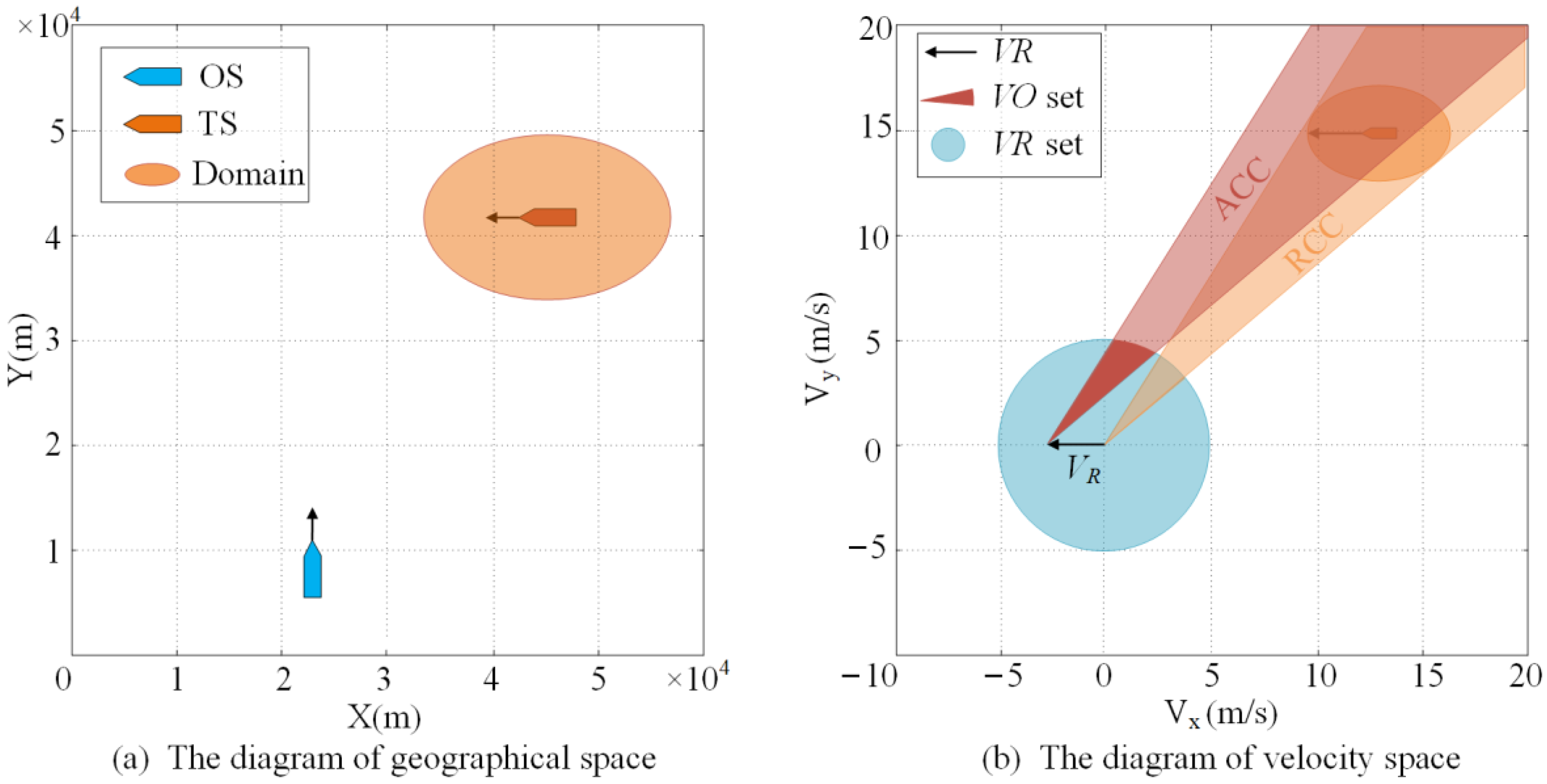
3.3. Velocity Obstacles Method

The VO method can be used to identify dangerous targets and find a direction to avoid them when the ship is sailing along the global path. The basic concept of the VO method was put forward by Fiorini (1998) [33], subsequently, it has been widely applied in many fields. In the shipping industry, the principle of the VO method is to project the motion characteristics between the ship and target from spatial-temporal space to velocity space and obtain the collision area, which is defined as the VO set from the perspective of velocity [6,34].

Assuming that the position and velocity of the ship are $X(t)$ and $V(t)$ at the time $t$, the motion of the ship can be expressed as:

$$P\left(t\right)=\left(X\left(t\right),V\left(t\right)\right)$$

(3)

Among them:

$$X\left(t\right)=\left(x,y\right)$$

(4)

$$V\left(t\right)=\left(v,c\right)$$

(5)

The own ship (OS) and target ship (TS) are $P_O(t)$ and $P_R(t)$, respectively. The relative velocity is defined as:

$$V_{OR}=V_O-V_R$$

(6)

Figure 3a shows the relative position of the OS (the blue ship) and TS (the yellow ship) in geographical space. The yellow area is the ship domain of the TS, denoted by $ConfP(P_R,R)$. Figure 3b is the velocity space of the OS, the blue circle is the velocity reachable (VR) set, and the yellow area RCC is made up of tangents between $ConfP(P_R,R)$ (the domain of TS) and $X_O(t)$ (the center point of VR set). It means the OS will enter the TS’s domain in the future when $V_{OR}$ falls in the RCC. The red area ACC can be obtained by moving the RCC along the $V_R$, it is equivalent to the $V_{OR}$ falls in RCC when $V_o$ falls in the ACC. Finally, the $VO$ set is obtained by finding the intersection of the $VR$ set, and ACC is shown as the crimson area in Figure 3b. There is collision risk between ships when the following condition is satisfied:

$$V_{OR}\in VO$$

(7)

The existence of collision risk between the OS and TS can be determined by judging whether the $V_O$ is within the VO set. However, the VO method cannot be directly applied to autonomous ships. On the one hand, the collision time $T$ can be calculated because the relative velocity $V_{OR}$ and the ship domain $ConfP(P_R,R)$ are known. There should be no collision risk when $T$ is more than Є, which is a time threshold for determining risk. However, it is judged that there is collision risk as long as $T$ exists in the typical VO method. The Є will be transformed into a circle of radius $R_{Є}$ and reflected in the velocity space of the OS to limit the collision time $T$ in this paper. On the other hand, the typical VO method is mainly used to judge collision risk between the OS and TS but cannot give a target course of collision avoidance. This paper will integrate COLREGS rules into the VO method to achieve the purpose of obtaining the target course.

3.4. Ship Motion and Control Models

It is well known that the motion of ships is highly nonlinear, therefore, this paper considered the ship’s characteristics via MMG and PID models. We can get the direction of avoiding collision through the VO method, and a local path can be obtained by combining the MMG and PID models. MMG is one of the models of ship motion simulation. The model was first proposed in Abkowitz (1964) [35] by a research group called the Maneuvering Modeling Group at the Japanese Towing Tank Conference (JTTC). The basic concept of the MMG model is to decompose the hydrodynamics, acting on the hull, propeller, and rudder, respectively, and then comprehensively analyze the interaction between each part so as to build a ship motion model. Compared with other models, the advantages of the MMG model lie in the fact that the hydrodynamic derivatives used in the model have explicit physical meanings, which is convenient for the clear understanding of a ship’s maneuvering motion [36].

As described by Yasukawa (2015) [37], the function of hydrodynamic action on the ship in the MMG model is as follows:

$$\{\begin{array}{l}X=\left(m+m_x\right)\dot{u}-\left(m+m_y\right)v_{m}r-x_{G}m{r}^2\\ Y=\left(m+m_y\right){\dot{v}}_m-\left(m+m_x\right)ur-x_{G}m\dot{r}\\ N_m=\left(I_{z}G+x_G^{2}m+J_z\right)\dot{r}+x_{G}m\left({\dot{v}}_m+ur\right)\end{array}$$

(8)

$X$,$Y$,$N_m$ are the surge force, lateral force, and yaw moment around midship. $m$,$m_x$,$m_y$ are the ship’s mass, added masses of the x-axis direction and y-axis direction. $u$,$v$,$v_m$ are the surge velocity, the lateral velocity at the center of attraction, and lateral velocity at midship. $x_G$ is the longitudinal coordinate of the center of the attractive force of the ship. $I_{z}G$ and $J_z$ are the moment of inertia of the ship and added moment of inertia. The specific hydrodynamic coefficient and solution method can be referred to Yasukawa (2015) [37].

Because the research object of this paper was an autonomous ship, the system of course control should also be considered. This paper adopted the classical PID navigation control system installed on most sea-going ships at present. Since the objective of the study focused more on the decision-making process of path planning, the control method of the autonomous ship was introduced to verify the feasibility of the proposed path planning algorithm. The parameters of the MMG model and PID model adopted in the subsequent experiments in this paper mainly referred to the program modified by Thor I. Fossen [38].

4. Model Design

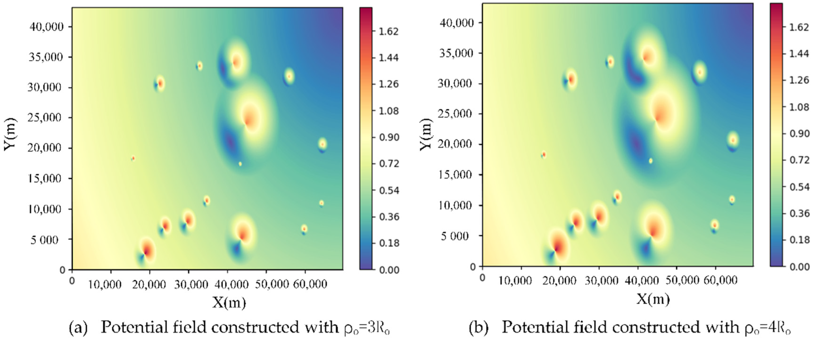
4.1. Map Construction

The first step for path planning is to construct the geographical environment map that includes obstacles and ships. Ships can be added to the geographical map with manual settings. Obstacles can be obtained by downloading the map from OpenStreetMap and extracted via QGIS.

For safety and convenience, the minimum circumscribed circle is used to replace the obstacle in the typical APF method, and the same treatment is also carried out in the improved APF method. In order to facilitate calculation, the point in the lower-left corner of the map is taken as the origin of the Cartesian coordinate system, and then the longitude and latitude information is transformed into fixed coordinate information. After the above steps, the geographical environment constructed is shown in Figure 4.

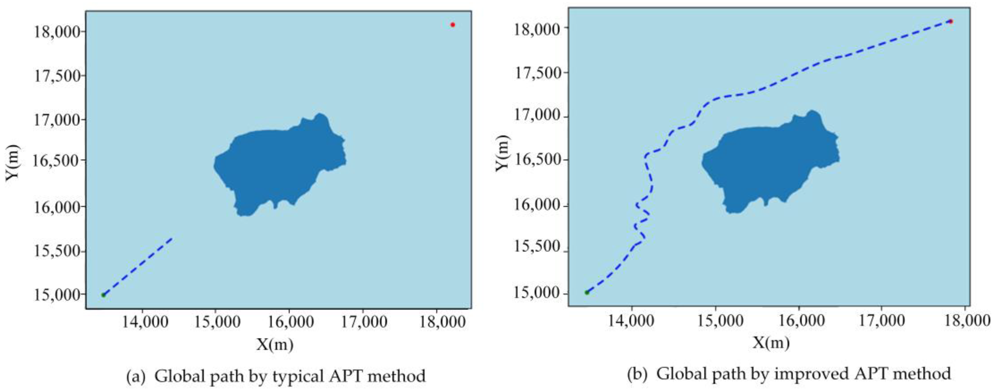
4.2. Global Path Planning with Improved APF Method

The purpose of this subsection is to introduce the improved APF method in detail and display the global path. The shortcomings of the typical APF method are an easy to fall into local optimum and too many turning points in the path obtained. Given the shortcomings of the traditional APF method, the following improvements were made.

The repulsive potential field was changed to avoid a local minimum. An extra force ${\overrightarrow{F}}_{extra}$ can be found to avoid falling into local minimization in which the attractive force ${\overrightarrow{F}}_{att}$ and repulsive force ${\overrightarrow{F}}_{rep}$ are on the same line and in opposite directions, as shown in Figure 5. By finding the minimum circumscribed circle of the obstacle, the center point $q_{obs}$ and radius $R_o$ of the circumscribed circle can be obtained. The circumscribed circle can be marked as $CirP(q_{obs},R_o)$. Two points can be obtained by making two tangent lines to $CirP(q_{obs},R_o)$ from the OS’s position $q$, and each of them can be used as a starting point for generating extra force. As shown in Figure 5, the direction of ${\overrightarrow{F}}_{extra}$ is the tangent line of the circumscribed circle starting from the OS and $\alpha$ is the included angle between ${\overrightarrow{F}}_{extra}$ and ${\overrightarrow{F}}_{att}$. The ${\overrightarrow{F}}_{extra}$ is expressed as follows:

$${\overrightarrow{F}}_{extra}=-grad\left(U_{\mathrm{extra}}(q)\right)=\{\begin{array}{l}-grad\left(\frac{1}{2}\mu {(\frac{1}{\rho (q,q_{\mathrm{extra}})}-\frac{1}{{\rho }_0})}^2\right) ,{\overrightarrow{F}}_{rep}=(-{\overrightarrow{F}}_{att})\\ 0 \hspace{1em}\hspace{1em}\hspace{1em}\hspace{1em}\hspace{1em}\hspace{1em}\hspace{1em}\hspace{1em}\hspace{1em}\hspace{1em},{\overrightarrow{F}}_{rep}\ne (-{\overrightarrow{F}}_{att})\end{array}$$

(9)

In the above Equation (9), $-grad$ represents the opposite direction of the gradient of the extra force, $\rho (q,q_{\mathrm{extra}})$ is the distance from point $q$ to point $q_{\mathrm{extra}}$, $\mu$ is gain of extra potential field, and equal to the gain of the repulsive potential field. The resultant force on the ship is as follows:

$$\overrightarrow{F}=\{\begin{array}{l}{\overrightarrow{F}}_{att}\hspace{1em}\hspace{1em}\hspace{1em}\hspace{1em}\hspace{1em},\rho (q,q_{obs})>{\rho }_0\\ {\overrightarrow{F}}_{rep}+{\overrightarrow{F}}_{att}\hspace{1em}\hspace{1em} ,\rho (q,q_{obs})\le {\rho }_0\\ {\overrightarrow{F}}_{extra}\hspace{1em}\hspace{1em}\hspace{1em}\hspace{1em} ,{\overrightarrow{F}}_{rep}=(-{\overrightarrow{F}}_{att})\end{array}$$

(10)

$\rho (q,q_{obs})$ is the distance from point $q$ to point $q_{obs}$. ${\rho }_0$ is the range of the repulsive potential field and generally related to the radius of the obstacle. When the resultant force on the ship is known, we can set a fixed step size and then continue to move along the direction of the resultant force to obtain the global path. As shown in Figure 6, the destination cannot be reached as shown in Figure 6a because the path falls into a local minimum when using the typical APF method. The APF method used in Figure 6b has been improved according to the above equations so that it can escape the local minimum to reach its destination.

The path obtained through the APF method has many turn points, as shown in Figure 6b. Changing the course frequently will increase the collision risk due to the poor maneuverability of ships. It is necessary to compress the global path using the trajectory compression method. Therefore, this paper adopted the DP algorithm to delete the turning points that only indicate small changes along the path and identified the turning points that follow the navigation practices. The pseudocode of the DP algorithm is shown in Algorithm 1, T is the candidate path that will be processed, function E(T(i), T(1), T(end)) means the shortest distance from the point T(i) to the line consisting of the first point T(1) and last point T(end), and ε which is the threshold of the DP algorithm, determines the level of compression. The DP algorithm is an iterative process until the path reaches the specified degree of compression. With this design, the global path that indicates the main turning points can be obtained with the integration of the APF and DP algorithms, as shown in Figure 7.

Algorithm 1. The pseudocode of the DP: pls(T,ε)
1	end = len(T)
2	dmax = 0
3	imax = 0
4	for i in range(2,end):
5	d = E(T(i), T(1), T(end))
6	If d > ε:
7	imax = i
8	dmax = d
9	if dmax > ε:
10	A = DP(T(1,imax), ε)
11	B = DP(T(imax,end), ε)
12	else:
13	return T(1,end)

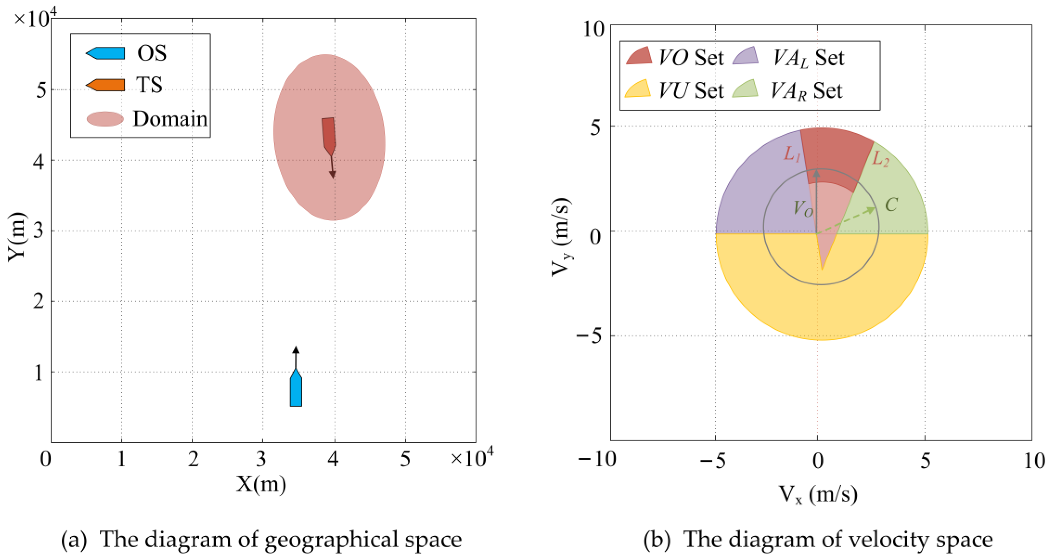
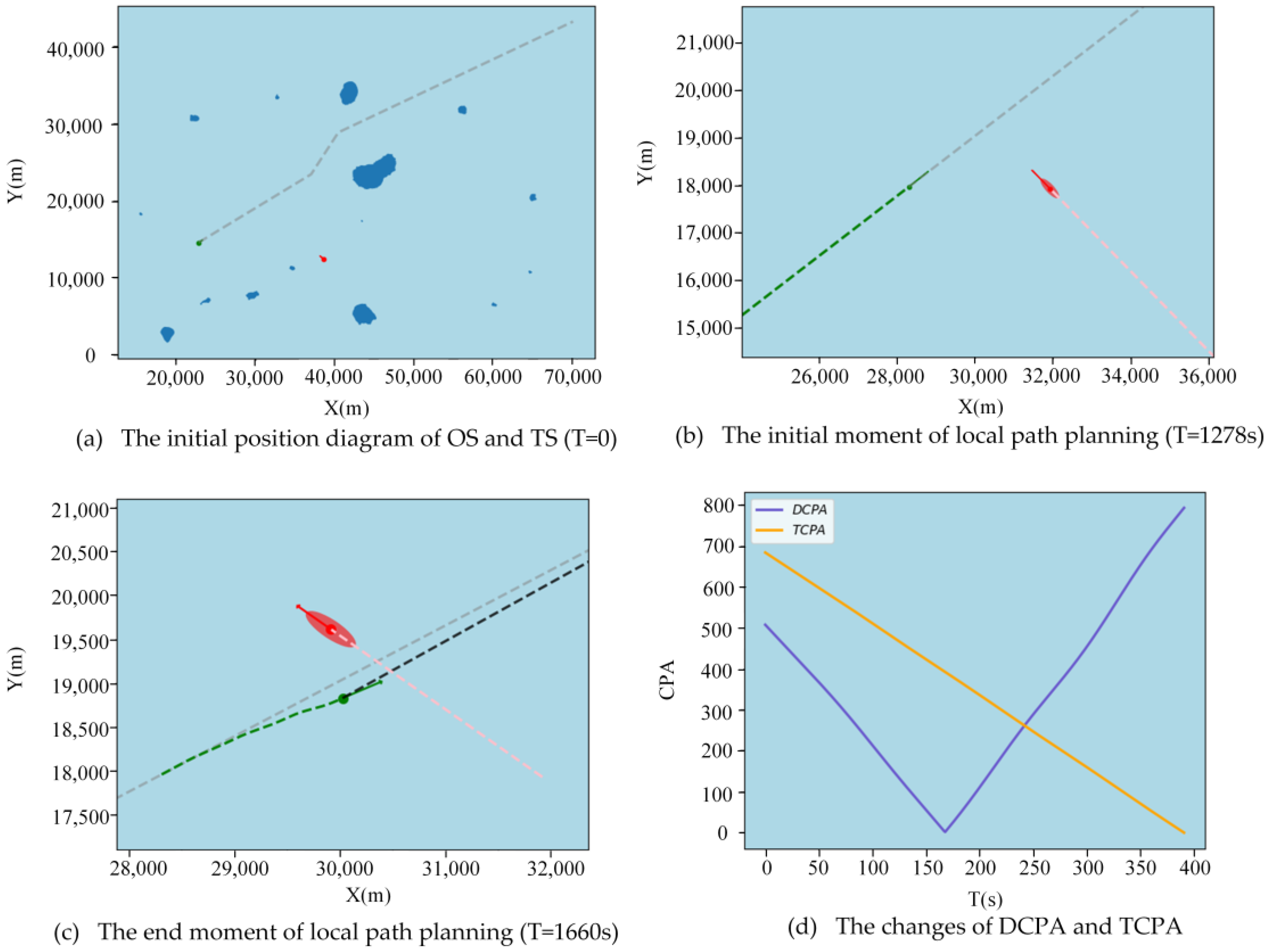
4.3. Local Path Planning with Modified VO Method

The global path cannot be directly utilized in the navigation process of autonomous ships as it does not provide detailed information on how to avoid collision. Therefore, detailed path planning, which is local path planning, should be performed. Local path planning is the process of identifying dangerous targets and avoiding them while sailing along the global path. This section will describe the details of the modified VO method and demonstrate its use to obtain a local path. The process of local path planning is divided into three stages: (1) identifying the collision risk, (2) calculating the direction of collision avoidance, and (3) obtaining the local path. We will introduce each stage herein.

Stage 1: Identifying the Collision Risk

The typical VO method can identify the collision risk from the perspective of the spatial dimension, but it can only calculate the probability of risk occurrence and ignore the urgency of risk. Therefore, we will set a time threshold to limit the collision time in which the ship enters the domain of the target ship and integrate it into the velocity space of the VO method after algebraic conversion. In navigation practice, seamen usually take CPA as the basis for judging collision risk between vessels. The algebraic method of solving DCPA and TCPA is as follows:

If the distance between the two vessels at time t is $D^{\left(t\right)}$:

$$\begin{array}{ll}{\left(D^{\left(t\right)}\right)}^2& ={\left[\left(x_R-x_O\right)+\left(v_R\cdot \sin c_R-v_O\cdot \sin c_O\right)\cdot t\right]}^2\\ & +{\left[\left(y_R-y_O\right)+\left(v_R\cdot \cos c_R-v_O\cdot \cos c_O\right)\cdot t\right]}^2\end{array}$$

(11)

If the above Equation (11) is substituted as follows:

$$\{\begin{array}{l}\Delta x=\left(x_R-x_O\right)\\ \Delta y=\left(y_R-y_O\right)\\ \Delta u=\left(v_R\cdot \sin c_R-v_O\cdot \sin c_O\right)\\ \Delta v=\left(v_R\cdot \cos c_R-v_O\cdot \cos c_O\right)\end{array}$$

(12)

Equation (12) above is simplified as:

$${\left(D^{\left(\mathrm{t}\right)}\right)}^2={\left(\Delta x+\Delta u\cdot t\right)}^2+{\left(\Delta y+\Delta v\cdot t\right)}^2$$

(13)

Take the derivative of Equation (13) with respect to t, and set the derivative equal to zero:

$$t=-\left(\Delta x\cdot \Delta u+\Delta y\cdot \Delta v\right)/\left(\Delta u^2+\Delta v^2\right)$$

(14)

TCPA is the t in the above Equation (14), and by replacing t in Equation (11), DCPA can be calculated. Now, assume that TCPA is equal to Є as the time threshold of collision. The Є will be transformed into a circle of radius $R_{Є}$, as shown in Figure 8. The $R_{Є}$ can be obtained as follows:

$$\alpha =\Delta x\left(v_O\cdot \sin c_O-\sin c_R\right)+\Delta y\left(v_O\cdot \cos c_O-\cos c_R\right)$$

(15)

$$\beta =\frac{\alpha }{Є}+2v_O\cdot \sin \left(c_R+c_O\right)$$

(16)

$$\{\begin{array}{l}{R}_{Є}=\sqrt{\frac{{\beta }^2}{4}-V_O^2}\pm \frac{\beta }{2}\\ 0\le R_{Є}\le V_{\max }\end{array}$$

(17)

where $V_{\max }$ represents the maximum velocity of OS.

As shown in Figure 8, the original VO set obtained by the typical VO method is divided into VO set1 and VO set2. This means the TCPA of two vessels will be less than threshold Є when the OS’s velocity falls in VO set1 such as V₁. Therefore, the VO set is equal to VO set1 when the time threshold is Є. There is no collision risk when velocity is in the VO set2. The risk of collision exists when the OS’s velocity satisfies the following equation:

$$V_O\in VO \mathrm{S}et1$$

(18)

Stage 2: Calculating the Direction of Collision Avoidance

The risk of collision between the two vessels already can be determined through the first stage. In this stage, we introduce how to calculate the direction of collision avoidance. This study had the following constraints on avoidance actions:

(1) Only consider avoiding the dangerous ship by changing direction since ships generally sail at constant speeds at sea.

(2) The feasible range of the direction change of the OS is restricted from 90° port to 90° starboard because using a U-turn or near U-turn to avoid collision will increase the risk of collision with other ships.

(3) The velocity reachable set of the OS will be divided into multiple sets, which set is used for avoidance is determined by COLREGS rules.

(4) According to COLREGS rules, a succession of small alterations of course and/or speed should be avoided; this paper takes the center of the avoidance set as the direction of collision avoidance.

(5) Only consider the situation where the OS is the give-way ship because the stand-on ship should maintain course and speed.

As shown in Figure 9, the velocity reachable set of the OS can be divided into VA_L set (purple area), VA_R set (green area), VU set (yellow area), and VO set (red area). VA_L set and VA_R set mean that the OS will turn left or turn right to avoid the collision. VU set will not be used as a standby avoidance area because of constraint (1).

Assuming that there is a risk of collision between the OS and TS, the OS will turn right to avoid the collision, denoted by the circle with radius $V_O$ as $ConfP(P_o,V_O)$ shown as the gray circle in Figure 9.

C₁ to C₂ is the turn set where the OS can take a right turn to avoid the collision, and the C₁ can be obtained as follows:

$$C_1=L2\oplus ConfP\left(P_o,V_O\right)$$

(19)

C₂ is equal to 90 because the feasible range of the avoidance course of the OS is restricted from 90° port to 90° starboard. The direction of collision avoidance can be obtained as follows:

$$C=\frac{C_1+C_2}{2}$$

(20)

According to rule 14 of the COLREGS rules, each vessel shall pass on the port side of the other when two vessels form a head-on situation. The OS will take the turn right to avoid the collision when the OS’s velocity falls in the VO set in the head-on situation, as shown in Figure 10. Figure 10a is the geographic space of the relative positions of the TS and OS in the head-on situation, and Figure 10b is the velocity space of the OS.

The crossing situation is shown in Figure 11. According to article 15 of the COLREGS rules, the vessel that has the other on her starboard side shall keep out of the way and shall avoid passing by the bow of the TS. Therefore, we will take avoidance action and pass by the stern of the TS when approaching on the starboard side, just as shown in Figure 11b.

The overtaking situation is shown in Figure 12. In accordance with article 13 of the COLREGS rules, this vessel shall be a give-way vessel when it is an overtaking vessel. But whether we should avoid from the left or the right in overtaking situations is not clear in the COLREGS rules. Therefore, we will compare the areas of VA_R set and VA_L set to determine which side has the greater avoidance space, shown as follows:

$$\{\begin{array}{l}C=C_R,\hspace{1em}\hspace{1em}\frac{{\mathrm{S}}_{{\mathrm{VA}}_{\mathrm{R}}}}{{\mathrm{S}}_{\mathrm{VAL}}}\ge 1\\ C=C_L,\hspace{1em}\hspace{1em}\frac{{\mathrm{S}}_{{\mathrm{VA}}_{\mathrm{R}}}}{{\mathrm{S}}_{\mathrm{VAL}}}<1\end{array}$$

(21)

Stage 3: Obtaining the Local Path

The direction of collision avoidance has been calculated through the above stages, and a local path conforming to ship maneuverability can be obtained by bringing the direction into the MMG and PID models. As shown in Figure 13, The red ellipse is the ship domain of the TS, and the green dotted line is the planned local path. The path is feasible because it takes COLREGS rules and ship characteristics into consideration. The endpoint of the local path is set to the point where TCPA is equal to 0 in this study.

5. Case Study

5.1. Case Design

In this section, a case study on path planning with the improved APF and modified VO methods is illustrated. To conduct the case study, an area was randomly chosen. Information was about the selected area is shown in

Table 1. Configuration of the geoinformation.

Item	Configuration
Boundary:	Latitude: 10.9391° N to 11.2667° N Longitude: 120.71° E to121.1543° E
Start point:	120.762° E/11.071° N
End point:	121.191° E/11.328° N
Origin of coordinate:	120.71° E/10.9391° N

. The obstacles in the selected area will be replaced by minimum circumscribed circles in Section 5.2 to construct the experimental scene. Two comparative experiments between the typical APF method and the improved APF method are described in Section 5.3 and prove that the improved APF method is better than the classical APF method in global path planning.

As shown in

Table 2. Configuration of the ship information.

Ship	Location	Speed (m/s)	Course (°)	Situation
OS	120.762° E/11.071° N	5	57
TS1	120.872° E/11.138° N	5	237	Head-on
TS2	120.905° E/11.051° N	6.7	167	Crossing
TS3	120.825° E/11.109° N	2	57	Overtaking

, in order to verify the feasibility of the modified VO method in different encounter situations, three ships were set up in this case study, and each TS constituted a different encounter situation from the OS. Three groups of experiments will be described in Section 5.4 for obtaining local paths in the different encounter situations.

5.2. Map Construction

Information about the case region is shown in Table 1. After downloading the vector map from OpenStreetMap and extracting it through QGIS, the information about the obstacles within the range was obtained. After converting the geographic coordinate system to a Cartesian coordinate system, the minimum circumscribed circles used to replace the obstacles are shown in

Table 3. Configuration of the minimum circumscribed circles.

Circles	Location (m)	Ro(m)	Circles	Location (m)	Ro (m)
Cir01	(15,703, 18,214)	208	Cir09	(43,259, 17,334)	148
Cir02	(18,838, 2589)	1037	Cir10	(43,597, 5022)	1525
Cir03	(22,404, 30,503)	572	Cir11	(44,764, 23,965)	2960
Cir04	(23,747, 6842)	713	Cir12	(55,805, 31,632)	578
Cir05	(29,629, 7694)	834	Cir13	(59,791, 6447)	348
Cir06	(32,730, 33,453)	338	Cir14	(64,252, 10,445)	18
Cir07	(34,584, 11,164)	373	Cir15	(64,276, 10,743)	235
Cir08	(41,623, 33,910)	1589	Cir16	(64,508, 20,377)	482

. The map selected is shown in Figure 14a, and the geographical environment constructed is shown in Figure 14b.

5.3. Global Path Planning

This section mainly describes two comparative experiments between the typical APF method and the improved APF method. The parameters of the typical and improved APF methods are shown in

Table 4. The parameters of the typical and improved APF methods.

Item	Start Point (m)	End Point (m)	λ	μ	${\mathit{\rho }}_0$	ε (m)	Step (m)
Typical APF	(28,419, 3016)	(53,046, 39,336)	1	1 × 105	3Ro/4Ro	/	200
Improved APF	(28,419, 3016)	(53,046, 39,336)	1	1 × 105	3Ro/4Ro	500	200

. λ and μ are gains of attractive potential and repulsive potential fields, the ratios of λ to μ will vary depending on the range of the environment. ${\rho }_0$ is the effective range of the repulsive potential field, which takes 3 and 4 times the radius of the obstacle, respectively. ε is the threshold of the DP algorithm, which determines the level of compression. The step size of APF is 200 m.

After the environmental data (shown in Table 3) and the parameters of the APF method (shown in Table 4) were known, the potential field map of the whole environment could be obtained. The potential field constructed by the APF method had changed with the range of the repulsion field ${\rho }_0$ change. Figure 15 a,b show the potential fields when ${\rho }_0$ is 3 times and 4 times the radius $R_o$ of the obstacle. The numbers on the right of each image indicate the addition of the vectors after the attractive and repulsive forces are normalized, respectively.

The following shows the use of the typical APF and improved APF methods, respectively, for global path planning under the above environmental conditions. As shown in Figure 16, the global paths planned by the typical APF method and improved APF method do not fall into a local minimum when ${\rho }_o=3R_o$. But the typical APF method falls into the local minimum when ${\rho }_o=4R_o$, while the improved APF method escapes from the local minimum, which proves that the improved APF method proposed in this paper is better than the typical APF method when dealing with local optimal problems.

From the above results, it can be seen that the improved APF method can avoid falling into a local minimum. Next, we compare the two methods from the perspective of the number of turn points and distance of the global path. As shown in Figure 17, the number of turning points and the distance of the path were greatly reduced when the effective range of the repulsive potential field ${\rho }_o$ equaled 4 times the radius of the obstacle, which is because the typical APF method fell into a local minimum.

As shown in Figure 17a, the improved APF method greatly reduced the number of turn points in the global path, making the global path conform to navigation practices. But the distance of the global path obtained with the improved APF was slightly less than that of the typical APF method, as shown in Figure 17b. In a nutshell, the improved APF method proposed in this paper can effectively make up for the local minimum of the typical APF method, and the global path obtained is more suitable for navigation practices.

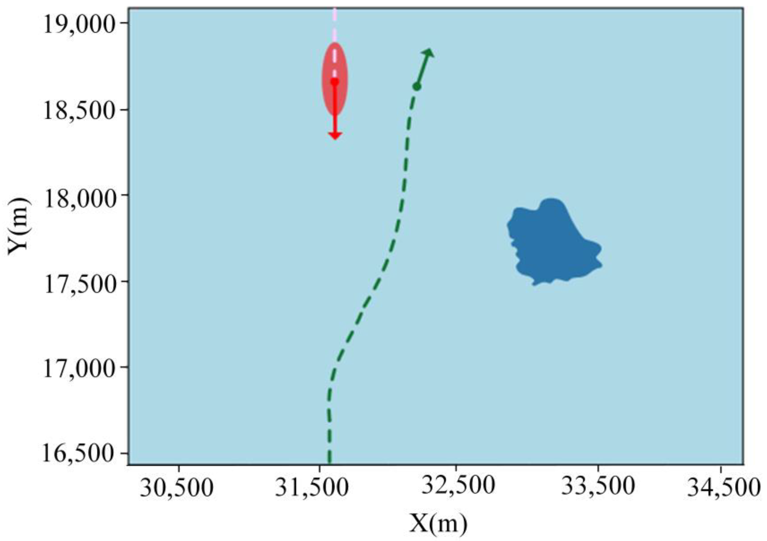
5.4. Local Path Planning

As shown in Table 2, we set up three target ships, each of which constituted a different encounter situation from the own ship and had a risk of collision. We used the modified VO method proposed in this paper to obtain the local paths for these different situations to prove the feasibility of the method.

Figure 18, Figure 19 and Figure 20 show the local avoidance process in head-on, crossing, and overtaking situations, respectively. Figure 18a, Figure 19a, and Figure 20a show the initial position diagrams of the OS (green) and TS (red), the gray dotted line is the global path obtained through the improved APF method. Figure 18b, Figure 19b, and Figure 20b show the initial moment of local path planning, that is, the first time the velocity of the OS falls within the VO set calculated by the modified VO model, and the green dotted line is the track of the OS and the red is the TS. Figure 18c, Figure 19c, and Figure 20c show the end moment of the local path planning in which the DCPA between the OS and TS is less than zero. The red ellipse is the ship domain of the TS, and the black dotted line is the global path after quadratic planning. Figure 18d, Figure 19d, and Figure 20d show the change of DCPA and TCPA in the process of local avoidance.

Figure 18 shows the local path planning under the head-on situation. There was no risk of collision between the OS and TS before 1023 s, so both ships sailing followed the planned route. The OS took a right turn to avoid the collision at 1023 s to 1458 s. In the whole local avoidance process, DCPA decreased first and then increased slightly, while TCPA kept decreasing until less than 0.

Figure 19 and Figure 20 show crossing situations and overtaking situations, respectively. In the crossing situation, the OS avoids collision by passing through the stern of the TS, while in the overtaking situation, the OS made a left turn to overtake from the port side of TS, both of which meet the requirements of the COLREGS rules. In the process of local avoidance, both TCPA showed a downward trend until less than 0, while the change of DCPA was different. In the crossing situation, TCPA first decreased and then increased because the two vessels first approached and then moved away, while in the overtaking situation, the two vessels kept getting closer, so DCPA showed a downward trend.

6. Conclusions

A hybrid path planning approach based on improved APF and modified VO methods for autonomous ships is proposed in this paper. The improved APF method corrects the shortcoming that typical the APF method will fall into the local minimum, and the turning point of the planned global path is smaller, which is more in line with navigation practices. When solving local path planning, this paper introduced a modified VO method that integrates COLREGS rules and the CPA model into the typical VO method, which can obtain local paths under different situations.

The geographical environment of the simulation experiment in this paper was constructed by extracting and processing the selected vector map data. Through comparative experiments, it was verified that the improved APF method is better than the typical APF method in dealing with the local minimum, and the global path produced is more in line with navigation practices. In addition, three encounter situations were set up to verify the feasibility of using the modified VO method to obtain local paths. The experimental results show that the local path obtained by this method can avoid target ships successfully, and the collision avoidance action is in accordance with COLREGS rules. In conclusion, the proposed method can provide a reference for future research on the path planning of autonomous ships.

However, the approach proposed in this paper still has some shortcomings. Before building the environment, we needed to download the vector map from other channels and carry out path planning after data processing, so we could meet the real-time requirements for the time being. The problem of path tracking was also not considered in this paper. After the local path planning, whether to sail according to the original global path or according to the second planned path and how to make the ship sail along the global path were not discussed in this paper. The authors will address the above shortcomings in subsequent research.

References

1. Chen, P.F.; Huang, Y.M.; Papadimitriou, E.; Mou, J.M.; van Gelder, P.H.A.J.M. An improved time discretized non-linear velocity obstacle method for multi-ship encounter detection. Ocean Eng. 2020, 196, 106718. [Google Scholar] [CrossRef]
2. He, J.; Hao, Y.; Wang, X.Q. An interpretable aid decision-making model for flag state control ship detention based on SMOTE and XGBoost. J. Mar. Sci. Eng. 2021, 9, 156. [Google Scholar] [CrossRef]
3. Li, M.X.; Mou, J.M.; He, Y.X.; Chen, L.Y.; Huang, Y.M. A rule-aware time-varying conflict risk measure for MASS considering maritime practice. Reliab. Eng. Syst. Saf. 2021, 215, 107816. [Google Scholar] [CrossRef]
4. Li, M.X.; Mou, J.M.; Chen, L.Y.; Huang, Y.M.; Chen, P.F. Comparison between the collision avoidance decision-making in theoretical research and navigation practices. Ocean Eng. 2021, 228, 108881. [Google Scholar] [CrossRef]
5. Yan, X.P.; Wang, S.W.; Ma, F.; Liu, Y.C.; Wang, J. A novel path planning approach for smart cargo ships based on anisotropic fast marching. Expert Syst. Appl. 2020, 159, 113558. [Google Scholar] [CrossRef]
6. Chen, P.F.; Huang, Y.M.; Eleonora, P.; Mou, J.M.; van Gelder, P.H.A.J.M. Global path planning for autonomous ship: A hybrid approach of fast marching square and velocity obstacles methods. Ocean Eng. 2020, 214, 107793. [Google Scholar] [CrossRef]
7. Marin-Plaza, P.; Hussein, A.; Martin, D.; Escalera, A.D.L. Global and local path planning study in a ROS-based research platform for autonomous vehicles. J. Adv. Transp. 2018, 2018, 6392697. [Google Scholar] [CrossRef]
8. Sarkar, R.; Barman, D.; Chowdhury, N. Domain knowledge based genetic algorithms for mobile robot path planning having single and multiple targets. J. King Saud Univ. Comput. Inf. Sci. 2020. [Google Scholar] [CrossRef]
9. Yu, X.B.; Li, C.L.; Yen, G.G. A knee-guided differential evolution algorithm for unmanned aerial vehicle path planning in disaster management. Appl. Soft Comput. 2021, 98, 106857. [Google Scholar] [CrossRef]
10. Aggarwal, S.; Kumar, N. Path planning techniques for unmanned aerial vehicles: A review, solutions, and challenges. Comput. Commun. 2020, 149, 270–299. [Google Scholar] [CrossRef]
11. Lyu, D.S.; Chen, Z.W.; Cai, Z.S.; Piao, S.H. Robot path planning by leveraging the graph-encoded floyd algorithm. Future Gener. Comput. Syst. 2021, 122, 204–208. [Google Scholar] [CrossRef]
12. Mou, J.M.; Li, M.X.; Hu, W.X.; Zhang, X.H.; Gong, S.; Chen, P.F.; Huang, Y.X. Mechanism of dynamic automatic collision avoidance and the optimal route in multi-ship encounter situations. J. Mar. Sci. Technol. 2020, 26. [Google Scholar] [CrossRef]
13. Premachandra, C.; Murakami, M.; Gohara, R.; Ninomiya, T.; Kato, K. Improving landmark detection accuracy for self-localization through baseboard recognition. Int. J. Mach. Learn. Cybern. 2017, 8, 1815–1826. [Google Scholar] [CrossRef]
14. Xie, L.; Xue, S.F.; Zhang, J.F.; Zhang, M.Y.; Tian, W.L.; Haugen, S. A path planning approach based on multi-direction A* algorithm for ships navigating within wind farm waters. Ocean Eng. 2019, 184, 311–322. [Google Scholar] [CrossRef]
15. Singh, Y.G.; Sharma, S.; Sutton, R.; Hatton, D.; Khan, A. A constrained A* approach towards optimal path planning for an unmanned surface vehicle in a maritime environment containing dynamic obstacles and ocean currents. Ocean Eng. 2018, 169, 187–201. [Google Scholar] [CrossRef] [Green Version]
16. Topaj, A.G.; Tarovik, O.V.; Bakharev, A.A.; Kondratenko, A.A. Optimal ice routing of a ship with icebreaker assistance. Appl. Ocean Res. 2019, 86, 177–187. [Google Scholar] [CrossRef]
17. Guo, H.; Mao, Z.Y.; Ding, W.J.; Liu, P.L. Optimal search path planning for unmanned surface vehicle based on an improved genetic algorithm. Comput. Electr. Eng. 2019, 79, 106467. [Google Scholar] [CrossRef]
18. Lim, H.S.; Fan, S.S.; Chin, H.K.H.; Chai, S.H.; Bose, N.; Kim, E. Constrained path planning of autonomous underwater vehicle using selectively-hybridized particle swarm optimization algorithms. IFAC-Pap. 2019, 52, 315–322. [Google Scholar] [CrossRef]
19. Candeloro, M.; Lekkas, A.M.; Sørensen, A.J. A voronoi-diagram-based dynamic path-planning system for underactuated marine vessels. Control Eng. Pract. 2017, 61, 41–54. [Google Scholar] [CrossRef]
20. Niu, H.L.; Savvaris, A.; Tsourdos, A.; Ji, Z. Voronoi-visibility roadmap-based path planning algorithm for unmanned Surface vehicles. J. Navig. 2019, 72, 850–874. [Google Scholar] [CrossRef]
21. Chang, K.Y.; Jan, G.E.; Su, C.M.; Parberry, L. Optimal interceptions on two-dimensional grids with obstacles. J. Navig. 2008, 61, 31–43. [Google Scholar] [CrossRef]
22. Wang, D.; Wang, P.; Zhang, X.; Guo, X.; Shu, Y.; Tian, X. An obstacle avoidance strategy for the wave glider based on the improved artificial potential field and collision prediction model. Ocean Eng. 2020, 206, 107356. [Google Scholar] [CrossRef]
23. Shin, Y.; Kim, E. Hybrid path planning using positioning risk and artificial potential fields. Aerosp. Sci. Technol. 2021, 112, 106640. [Google Scholar] [CrossRef]
24. Nakajima, K.; Premachandra, C.; Kato, K. 3D environment mapping and self-position estimation by a small flying robot mounted with a movable ultrasonic range sensor. J. Electr. Syst. Inf. Technol. 2017, 4, 289–298. [Google Scholar] [CrossRef]
25. Demirhan, M.; Premachandra, C. Development of an automated camera-based drone landing system. IEEE Access 2020, 8, 202111–202121. [Google Scholar] [CrossRef]
26. Premachandra, C.; Thanh, D.N.H.; Kimura, T.; Kawanaka, H. A study on hovering control of small aerial robot by sensing existing floor features. IEEE/CAA J. Autom. Sin. 2020, 7, 1016–1025. [Google Scholar] [CrossRef]
27. Guo, S.Q.; Mou, J.M.; Chen, L.Y.; Chen, P.F. Improved kinematic interpolation for AIS trajectory reconstruction. Ocean Eng. 2021, 234, 109256. [Google Scholar] [CrossRef]
28. Wang, X.Y.; Feng, K.; Wang, G.; Wang, Q.Z. Local path optimization method for unmanned ship based on particle swarm acceleration calculation and dynamic optimal control. Appl. Ocean Res. 2021, 110, 102588. [Google Scholar] [CrossRef]
29. Yang, R.W.; Xu, J.S.; Wang, X.; Zhou, Q. Parallel trajectory planning for shipborne Autonomous collision avoidance system. Appl. Ocean Res. 2019, 91, 101875. [Google Scholar] [CrossRef]
30. He, Y.X.; Jin, Y.; Huang, L.W.; Xiong, Y.; Chen, P.F.; Mou, J.M. Quantitative analysis of COLREG rules and seamanship for autonomous collision avoidance at open sea. Ocean Eng. 2017, 140, 281–291. [Google Scholar] [CrossRef]
31. Khatib, O. Real-time obstacle avoidance for manipulators and mobile robots. Int. J. Robot. Res. 1986, 5, 90–98. [Google Scholar] [CrossRef]
32. De Vries, G.K.D.; Van Someren, M. Machine learning for vessel trajectories using compression, alignments and domain knowledge. Expert Syst. Appl. 2012, 39, 13426–13439. [Google Scholar] [CrossRef]
33. Fiorini, P.; Shiller, Z. Motion planning in dynamic environments using velocity obstacles International. J. Robot. Res. 1998, 17, 760–772. [Google Scholar] [CrossRef]
34. Chen, P.F.; Li, M.X.; Mou, J.M. A velocity obstacle-based real-time regional ship collision risk analysis method. J. Mar. Sci. Eng. 2021, 9, 428. [Google Scholar] [CrossRef]
35. Abkowitz, M.A. Lectures on Ship Hydrodynamics–Steering and Maneuverability; Report Hy-5; Hydro–og Aeordynamisk Laboratorium: Lyngby, Denmark, 1964. [Google Scholar]
36. Zhang, C.L.; Liu, X.J.; Wan, D.C.; Wang, J.B. Experimental and numerical investigations of advancing speed effects on hydrodynamic derivatives in MMG model, part I: Xvv,Yv,Nv. Ocean Eng. 2019, 179, 67–75. [Google Scholar] [CrossRef]
37. Yasukawa, H.; Yoshimura, Y. Introduction of MMG standard method for ship maneuvering predictions. J. Mar. Sci. Technol. 2015, 20, 37–52. [Google Scholar] [CrossRef] [Green Version]
38. Fossen, T.I. Handbook of Marine Craft Hydrodynamics and Motion Control, 1st ed.; Wiley: Hoboken, NJ, USA, 2011. [Google Scholar]
Figure 1. Flowchart of the research methodology.
Jmse 09 00761 g001
Figure 2. The potential field as constructed via the APF method.
Jmse 09 00761 g002
Figure 3. The diagram of the VO method.
Jmse 09 00761 g003
Figure 4. Example of map constructed.
Jmse 09 00761 g004
Figure 5. The diagram of the improved repulsive potential field.
Jmse 09 00761 g005
Figure 6. Example of global paths by typical and improved AFP methods.
Jmse 09 00761 g006
Figure 7. Example of global paths before and after compression.
Jmse 09 00761 g007
Figure 8. The diagram of VO set by the modified VO method.
Jmse 09 00761 g008
Figure 9. The diagram of the modified VO method.
Jmse 09 00761 g009
Figure 10. The direction of collision avoidance in a head-on situation.
Jmse 09 00761 g010
Figure 11. The direction of collision avoiding in a crossing situation.
Jmse 09 00761 g011
Figure 12. The direction of collision avoidance in an overtaking situation.
Jmse 09 00761 g012
Figure 13. The diagram of the local path.
Jmse 09 00761 g013
Figure 14. Constructed environment map.
Jmse 09 00761 g014
Figure 15. The potential field constructed with the improved APF method.
Jmse 09 00761 g015
Figure 16. The global paths with the typical APF and improved APF methods.
Jmse 09 00761 g016
Figure 17. The comparison of the turn points and distance.
Jmse 09 00761 g017
Figure 18. The local path planning during the head-on situation.
Jmse 09 00761 g018
Figure 19. The local path planning during the crossing situation.
Jmse 09 00761 g019
Figure 20. The local path planning during the overtaking situation.
Jmse 09 00761 g020