Numerical Study on Interaction between Submarine Landslides and a Monopile Using CFD Techniques

Abstract

Offshore installations with pile foundations in shallow water are vulnerable to submarine landslides, which cause serious damage to engineering facilities, loss of life, and loss of money. Due to a shortage of real observation data and the difficulty of reproduction, we lack insight into the interaction behavior between submarine landslides and monopiles. This study capitalized on ANSYS Fluent 20.0 to develop a three-dimensional biphasic (water and slurry) numerical model. This CFD model was used to analyze the interaction between a monopile and submarine landslides at different flow heights. The velocities of submarine landslides were from low to high values. Two modes of interactional forces acting on the monopile are proposed, which are (i) interaction force with peak value and (ii) interaction force without peak value. The influence of flow height and velocity on interaction forces was investigated. Results show that the effect of the flow heights on the interaction force is significant at low velocity stage, while the peak force representing a hazard level of the pile was non-negligible under high flow velocity and low flow height conditions, which should be considered in a future study. The related mechanisms are revealed with a hybrid model considering different components of the force.

1. Introduction

With the increasing exploitation of offshore resources, many offshore installations have been put into use, such as fixed platforms, submarine pipelines, and other subsea facilities [1]. These installations may be exposed to the devastating threats of submarine landslides, which are a common and frequent marine geohazard [2,3]. Submarine landslides may be triggered by many factors [4], such as volcanoes and earthquakes, waves, dissociation of hydrate methane, and so on. Among them, storm surge is a very possible trigger mechanism in shallow water area [5,6,7]. Under the influence of wave dynamic loading of the storm surge, seabed instability may happen in this area [8]. When the seabed becomes unstable, submarine landslides can gradually disintegrate into fluidized debris flows [9], with velocity up to 20 m/s [10,11,12,13], which have the potential to severely damage structures along the paths. This type of hazard usually causes injury or loss of life and imposes significant additional project costs for mitigating their effects [14,15,16]. In shallow water areas, piles are widely used as foundation for engineering structures [1,17,18]. To ensure the safety of design and operation of offshore structures with pile foundations, estimating the potential interaction force between submarine debris flows and a monopile is of great research significance and practical value for marine engineers.

Recently, a large number of studies on submarine landslide–structure interaction have been carried out. Among them, the interaction between the submarine landslides and pipelines have particularly attracted researchers’ attention. In these studies, the major focus is the debris flow stage of submarine landslides, which has the potential for catastrophic disasters to seafloor structures. For the debris flow stage, fluid mechanics principles seems to be more appropriate [10,19,20]. Based on these theoretical principles, flume tests were performed to estimate the interaction force acting on pipelines, which lays the foundation in this research field [21]. Then CFD analyses [22] were conducted to complement the flume tests results. The data of CFD calculations combined with the results from the flume tests are meant to propose the relationship between the drag force coefficient and Reynolds number. Next, some researchers extended the previous works to study the normal and longitudinal interaction forces at different impact angles of submarine debris flows [23,24,25]. Afterwards, more factors on the drag force, such as suspension height [26,27,28], temperature of submarine debris flows [29], shape of the pipeline [30,31,32], strain-softening effects on soil strength [33], were also considered. In addition, some studies [34,35] used the material point method to investigate impact forces on pipelines, while an explanation of the mechanism of peak force was provided by [36,37].

It should be noted that previous studies mainly focused on the interaction force acting on pipelines, which is different from that acting on a pile. Feng et al. [38] launched a small number of flume tests to investigate the interaction force acting on a monopile at moderate flow velocities (0.38–0.94 m/s) through preliminary research. However, due to the limitation of the Feng’s experiment, tests in high-speed and low-speed movement of submarine landslides were not considered. Moreover, in offshore environments, flow heights of submarine debris flow have a remarkable influence on the force acting on a monopile, and the effect of flow heights has not been discussed in the flume tests. The understanding of the interaction processes and underlying mechanism is still inadequate due to insufficient data.

In this paper, a three-dimensional biphasic (slurry and water) numerical model using ANSYS Fluent 20.0 was developed. This model, based on the Herschel–Bulkley rheology, was used to investigate the interaction between submarine debris flows and a monopile. Firstly, the numerical model was verified by the results of a flume test. Then, a large number of simulations were carried out and two models of interaction force are summarized. The effects of flow velocities and flow heights on interaction forces on the monopile are also discussed. A qualitative variation law of the interaction force is proposed and the mechanism underlying is revealed through a hybrid model considering different components of the force. In addition, the difference between the peak and the stable drag coefficients is discussed to estimate the influence of the peak value, which is highly harmful for a monopile.

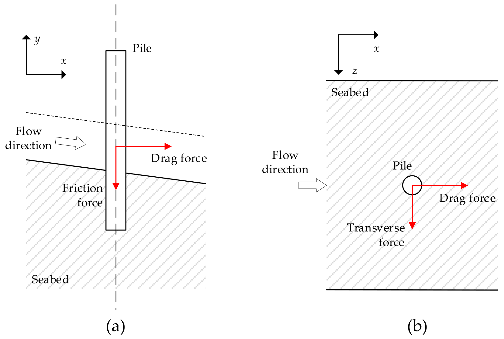
2. Interaction Model

In shallow water areas, after the seabed failure is triggered by large waves, submarine landslides may flow downslope. In this process, the submarine landslide body may evolve into submarine debris flows, which have greater influence and larger potential damage for marine structures. The present research mainly focus on the submarine debris flow stage, where the landslide body material may be considered as a fully remolded viscous fluid [9,39]. The interaction force between submarine debris flows and the monopile plays a vital role in the safety of offshore installations. In this study, due to the complexity of the interaction force in the underwater environment, the simulation just focuses on the force acting on the monopile. The monopile was fixed on the seabed slope whose surface was a rough wall boundary. Moreover, it is assumed that the monopile does not deform when interacting with submarine debris flows, as shown in Figure 1. This is therefore an upper bound of the loading scenario; that is, the estimation of the interaction force is relatively safe.

The interaction force of submarine debris flows acting on a monopile is divided into three components: drag force (normal), friction force (axis), and transverse force (lateral). The primary concern in this study is the drag force, which represents the most detrimental load. For the fluidized debris flow stage, the drag force exerted by the submarine debris flows and water on the monopile was calculated in the simulations using the fluid dynamics method, which is simpler and more popular [40],. Therefore, the drag force coefficient, C_D, is defined in the same way as that in Zakeri et al. [24].

$$C_D=\frac{F_D}{\frac{1}{2}\rho U_{\infty }^{2}A}=\frac{F_D}{\frac{1}{2}\rho U_{\infty }^{2}DH}$$

(1)

where C_D, ρ and D are the drag force coefficient, the density of a submarine debris flows, and the diameter of a monopile, respectively. A is the normal projected frontal areas of a monopile. H is the flow height of submarine debris flows. U_∞ is the approaching velocity of the submarine debris flows head, which was taken as the flow velocity of submarine debris flows. This is because when hydroplaning occurs, the submarine debris flows head advances as a plug flow with a uniform velocity profile [24]. F_D is the measured total drag force. For the Reynolds number of the submarine debris flows (Re_{non-Newtonian}), the definition, with τ as the shear stress of the submarine debris flows, is given by Equation (2).

$$R{e}_{non-Newtonian}=\frac{\rho U_{\infty }^2}{\tau }$$

(2)

3. Numerical Research Methods

3.1. General

Currently, many numerical methods, which can deal with large deformation problems, are available for simulating the post-failure runout of submarine landslides. Such numerical methods include: the coupled Eulerian–Lagrangian method (CEL) [41], mesh-based large-deformation finite element analysis (LDFE) [42], meshless material point method (MPM) [35], smoothed particle hydrodynamics (SPH) [43,44], computational fluid dynamics with the discrete element method (CFD-DEM) [45], and so on. Among them, computational fluid dynamics (CFD) is one of the most widely used numerical methods [46,47,48,49,50]. The validity of a numerical method for calculating the impact of submarine debris flows on pipelines has been successfully demonstrated by using CFD [22,23,24,36,51]. The CFD software ANSYS Fluent 20.0 (Ansys student 2020 R2 (Built-in license valid until 7/31/21).) was employed in this study, which is a general-purpose CFD software that includes solver based on the finite volume method (FVM) for unstructured meshes.

The submarine debris flows constitutes an incompressible biphasic (slurry and water) flow regime. As such, the Eulerian multiphase model is used to simulate the constant-speed fluidized submarine debris flows interacting with a monopile. In the numerical model, conservation equations of mass and Navier–Stokes equations method are discretized using the FVM. They are solved separately for each phase. The interphase coupling is achieved through the shared pressure and interphase exchange coefficients. A general descriptions of the theory and associated formulations regarding Eulerian multiphase model used to analyze the result can be found in the ANSYS Fluent Theory Guide [52].

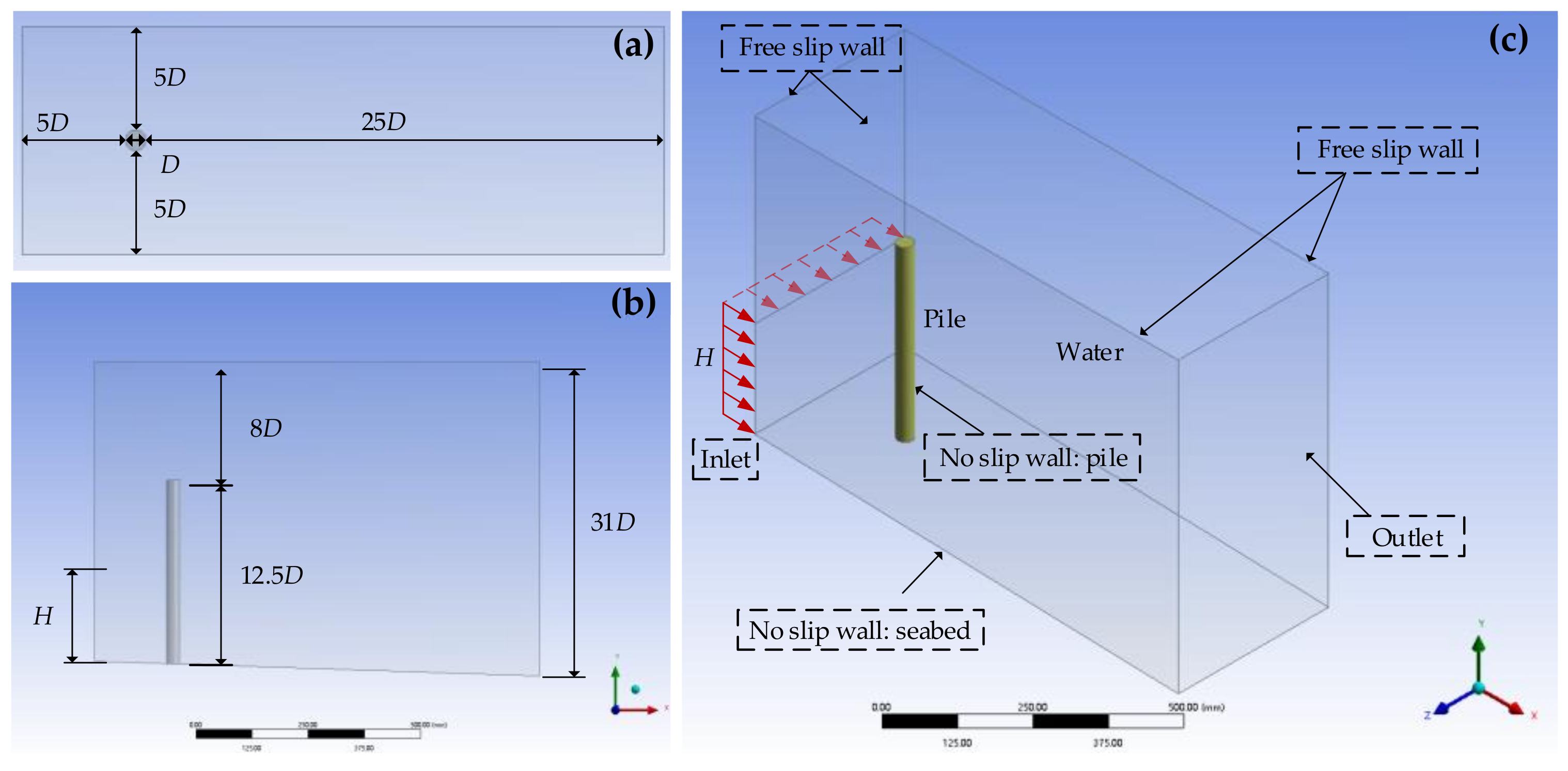
3.2. CFD Model Setup

Feng’s experimental data [38] were complemented using a similar CFD model by simulating mudflow entering the domain full of water at various flow velocities and heights. Parameters of submarine debris flows in the numerical model was strictly within the applicable range, which does not affect the fundamental understanding of the qualitative variation law and mechanism underlying [36,53]. The numerical model used to simulate the submarine debris flows-pile interaction is shown in Figure 2. The pile diameter (D) used in the simulations was 32 mm. The domain is 11D wide, 31D long, and the maximum height is 31D at the shallowest point (i.e., at the outlet). The slope angle of seabed is set as 4 degree. Figure 2b shows the pile is 12.5D high, whose top surface is 8D away from the top boundary of the domain. The monopile was more than 5D away from all the boundaries of the domain, which was found through sensitivity studies to be sufficient to eliminate boundary effects.

Both the monopile and seabed surfaces were modeled as rough no slip boundary conditions with the equivalent sand-grain roughness, k_s, of 1.6 × 10⁻⁶ m [54] and 12.5 × 10⁻⁶ m [38], respectively. The submarine debris flows of different flow heights (H) entered from the left side of the domain, with a constant velocity parallel to the seabed, as depicted in Figure 2c. The top and both sides of the domain as well as the wall above the inlet were modeled as free-slip wall boundary condition, which reduces the computation time required to compute the water flow field on these surfaces without affecting the submarine debris flows [24]. The outlet was modeled as outflow boundary condition.

The domain is discretized into unstructured meshes using the ANSYS Meshing module, as shown in Figure 3. The average maximum mesh size was 3.5 × 10⁻² m. Since submarine debris flow-pile interaction is of main interest for the study of fluid–structure interaction, meshes around the monopile were refined to a maximum mesh size of 0.01 m. The inflation boundary of five layers with growth rate of 1.2 was set at the pile edge. The maximum mesh size on the monopile surface was 2.5 × 10⁻³ m and gradually increased to 0.01 m within the 3D outward radial distance. Through the mesh sensitivity analysis, a mesh of 390,000 magnitude was confirmed for the calculation to balance the computational efficiency and accuracy, as shown in Figure 4.

The domains were set up for two-phase flow. The Herschel–Bulkley rheological properties of the submarine debris flows in the flume experiments given in

Table 1. Composition and rheological properties of submarine debris flows adapted from Feng et al. [38].

Submarine Landslide	Mass Fraction (%)			Herschel–Bulkley Rheological Model				Density (kg/m3)
	Clay	Water	Sand	τy (Pa)	K (Pa·sn)	n	R2
15% Clay	15	50	35	0.50	1.50	0.42	0.987	1763
20% Clay	20	45	35	1.80	1.40	0.54	0.976	1774
25% Clay	25	40	35	3.70	1.20	0.60	0.979	1788
30% Clay	30	35	35	5.90	0.90	0.87	0.986	1796

Note: the Herschel–Bulkley model is expressed with τ = τ_y + Kγⁿ. τ is the shear stress, τ_y is the yield stress, K is the consistency index, n is the flow behavior index and γ is the shear rate.

and standard properties of water were used in the simulations, respectively. Turbulence generated in the two-phase flow was simulated using the κ-ω model. The difference between two-phase flow velocities produces phase interaction at the contact surface. The phase interaction was set as drag coefficient. The total time of simulation was 3–10 s (related to mud velocity), and the time step was 0.0005 s. The transient formulation and spatial discretization were taken as the second order form.

3.3. Comparison and Validation

To verify the validity and reliability of the numerical calculations, various operating conditions of Feng’s study [38] were simulated. Figure 5 shows the comparison between the current calculations and previous results. Generally speaking, the current drag force coefficients are quite similar to the results obtained in the flume tests. The simulation yielded higher drag force coefficients than that in the experiment at low Re_{non-Newtonian}. The reason for this discrepancy is that the mudflow slightly slip on some parts of the pile in the flume experiment, whereas no slippage is allowed in the numerical simulation. As for high Re_{non-Newtonian}, the numerical results are lower than the experimental data. This may be due to the large discreteness of experimental results [30].

4. Results and Discussion

4.1. Load Characteristic of the Pile

The simulations were extended to include the full range of flow velocities. The effect of different flow heights on the drag force was systematically studied. The rheological parameters and the seabed slope utilized in all of the simulations were the same as the ones used in the flume experiments. The ranges of submarine debris flow parameters used in the simulations are shown in

Table 2. Ranges of submarine debris flow parameters used in simulation.

Parameter	Value
Rheological model	Submarine debris flow of 20% clay in Table 1
Flow height, H	D, 3D, 5D, 7D, 9D
Flow velocity of the inlet, U∞	0.1, 0.15, 0.2, 0.25, 0.3, 0.35, 0.4, 0.45, 0.5, 0.6, 0.75, 1, 1.25, 1.5, 1.75, 2, 2.5 m/s

. A total of 85 CFD simulations were conducted.

Figure 6 shows a typical loading response imposed by submarine debris flows on the monopile. For low U_∞ and H, no peak drag force is observed. When U_∞ and H increase, the peak value appears. Two typical models can be summarized from all the simulations conducted, which are model 1 (high U_∞, H) with a peak drag force value and model 2 (low U_∞, H) without a peak drag force value. We take submarine debris flows with U_∞ = 0.3 m/s, H = D (see curve model 2 in Figure 6) and U_∞ = 1.25 m/s, H = 5D (see curve model 1 in Figure 6) as two examples to illustrate both models. For model 1, the drag force increases with time sharply up to point A₁ and then decreases to a negative value. Then the value quickly rises to a peak at point C₁, and afterwards gradually declines until it reaches a stable value at point D₁. For model 2, the stage before point B₂ is similar to model 1. After point B₂, the drag force gradually increases to a stable value at point C₂.

The formation mechanism of the models is explained as follows. At point A₁ and A₂, the landslide body with a certain initial velocity enters the domain from the inlet and pushes the seawater in front so that the originally stationary seawater begins to accelerate to a higher velocity and first impacts the monopile, causing a sharp increase of the force [31]. As the landslide moves forward, the left end and right ends of the pile can be divided into upstream and downstream zones. For model 1, before the debris flows touch the monopile, strong vortices form upstream of the pile, resulting in a negative pressure zone. This slows down the growth of the drag force before point B₁, as shown in Figure 7a. After the landslide body gradually comes into contact with the monopile, the pressure difference between the positive pressure zone and the negative pressure zone increases and the drag force gradually increases to its peak value, as shown in Figure 7b. As more of the landslide body engulfs the monopile, the negative pressure zone becomes narrower. The drag force decreases to the stable value, as shown in Figure 7c. For model 2, since the velocity and flow height are lower, it takes longer for the landslide body to meet with the monopile at point B₂ and the drag force is smaller than that of model 1, as shown in Figure 7d. It can be seen from Figure 7e that drag force increases to the stable immediately after point B2 because the pressure difference between the upstream and downstream zones is negligible. Generally, in addition to the velocity of submarine debris flows, the flow height influences the drag force acting on the monopile. Therefore, it is necessary to perform a detailed analysis to reveal the underlying law and mechanism.

4.2. Influence of the Submarine Debris Flow Heights

Considering the different flow heights (H), the computed drag force was analyzed utilizing the same method as described in Section 2. Figure 8 shows the relationship between C_D and Re_{non-Newtonian} at different H. The peak drag force coefficient (C_D-P) and the stable drag force coefficient (C_D-S) decrease with Re. A critical Reynolds number (Re_c = 165.5, U_∞ = 1 m/s) is observed. The overall trend at low Reynolds number stage (Re_{non-Newtonian} < Re_c) and high Reynolds number stage (Re_{non-Newtonian} > Re_c) are different.

Figure 9a shows that at the lower Reynolds number stage (Re_{non-Newtonian} < Re_c), C_D-P increases with H and reaches the maximum value at H = 9D. C_D-P remains almost constant and the gradient of C_D-P equals to zero, when Re_{non-Newtonian} = Re_c. When Re_{non-Newtonian} > Re_c, C_D-P decreases with H to a minimum at H = 9D. Referring to Figure 9b, C_D-S gives a similar trend as that of C_D-P at the lower Reynolds number stage (Re_{non-Newtonian} < Re_c). However, C_D-S for the full range of heights remains the same after Re_{non-Newtonian} is greater than Re_c. In addition, the gradient of C_D along with H when Re_{non-Newtonian} < Re_c is greater than that of higher Re_{non-Newtonian}, and when Re_{non-Newtonian} > Re_c, the gradient of C_D is much smaller than that of the lower Reynolds number range. In short, the effect of H on C_D is significant at the lower Reynolds number stage (Re_{non-Newtonian} < Re_c).

According to the formation mechanism [35], the drag force is composed of the differential pressure inertia force, the viscous strength force and the static pressure force. The viscous strength force is closely related to the roughness of the monopile surface and the debris flows movement within the boundary layer. However, since the same flow model is used in this study and the roughness of the monopile is consistent in all simulations, the contribution of the viscous strength force is not considered. For low Re_{non-Newtonian} conditions, the static pressure force closely related to the flow height (H) is dominant. Therefore, the drag force increases with H. For high Re_{non-Newtonian} conditions, the static pressure force is negligible, hence the differential pressure inertia force, which is due to the separated region of the monopile, is considered [30]. Figure 10 compares the mud volume fraction and pressure distribution of the same submarine debris flow with the same high impacting velocity at the time of the peak drag force. At this moment, the shape of the downstream zone for H = D is significantly different from those for H = 5D and 9D, resulting in the different separated region. The separated region has a direct influence on the negative pressure zone, which leads to the variation of the differential pressure inertia force.

To understand the quantitative variation of the drag coefficients, the maximum rate of change of C_D (β) with different H is obtained, as shown in Figure 11. When Re_{non-Newtonian} < Re_c, β of C_D-P is greater than that of C_D-S. The maximums of C_D-S and C_D-P are 54% and 91%, respectively. Basically, the influence of H on C_D-P is greater than C_D-S, and the difference between C_D-P and C_D-S should be elaborated.

4.3. Influence of Peak and Stable Drag Force Coefficients

Figure 12 shows the variation of the residual of drag force coefficients (R) with respect to Re_{non-Newtonian}. The overall trend shows that R decreases with Re_{non-Newtonian} until it reaches a critical value at Re_C = 165.5, and then begins to increase. For H = D, when Re_{non-Newtonian} < 20, R is close to 1, indicating that the influence of H is negligible, which is consistent with the law of model 2. The focus in this study falls within the low Re_{non-Newtonian} range (Re_{non-Newtonian} < Re_c) because of the significant impact on C_D. When Re_{non-Newtonian} < 100, a greater H of submarine debris flow corresponds to a greater R, which means a greater gap between the peak drag force and the stable drag force. However, considering the flow height (H), the variation law of R in the middle Re range (100 < Re_{non-Newtonian} < 250) is opposite that in the lower Re range (Re_{non-Newtonian} < 100). For the middle Re, the minimum (R = 0.638) appears at H = D, which the means peak drag force is more significant with higher Re_{non-Newtonian} and lower H. In a previous study [38], due to the limitation of the tests, the stable drag force, which lasts a relatively long period, was selected to analyze the drag force. However, the present study shows the peak drag force is significant and highly harmful for the pile.

5. Conclusions

In this paper, the interaction force between submarine debris flows and a monopile was systematically analyzed with computational fluid dynamics (CFD). To complement flume experiment data, flow velocities of the submarine debris flows were varied in the range of 0.1–2.5 m/s. Moreover, the effect of the flow height was carefully investigated. The main conclusions are as follows.

(1)

The numerical results agreed well with the experimental results. Therefore, such a CFD method may be utilized to investigate the interaction between the submarine debris flows and a monopile with similar settings.

(2)

The typical load characteristics of the drag force acting on the monopile were analyzed. Two modes of the drag force were proposed. The flow velocity and the flow height of submarine debris flows were found to have an influence on the mode of the drag force. The underlying mechanism was revealed using a hybrid model combining the effects resulting from submarine debris flows differential pressure inertia force, viscous strength force and static pressure force.

(3)

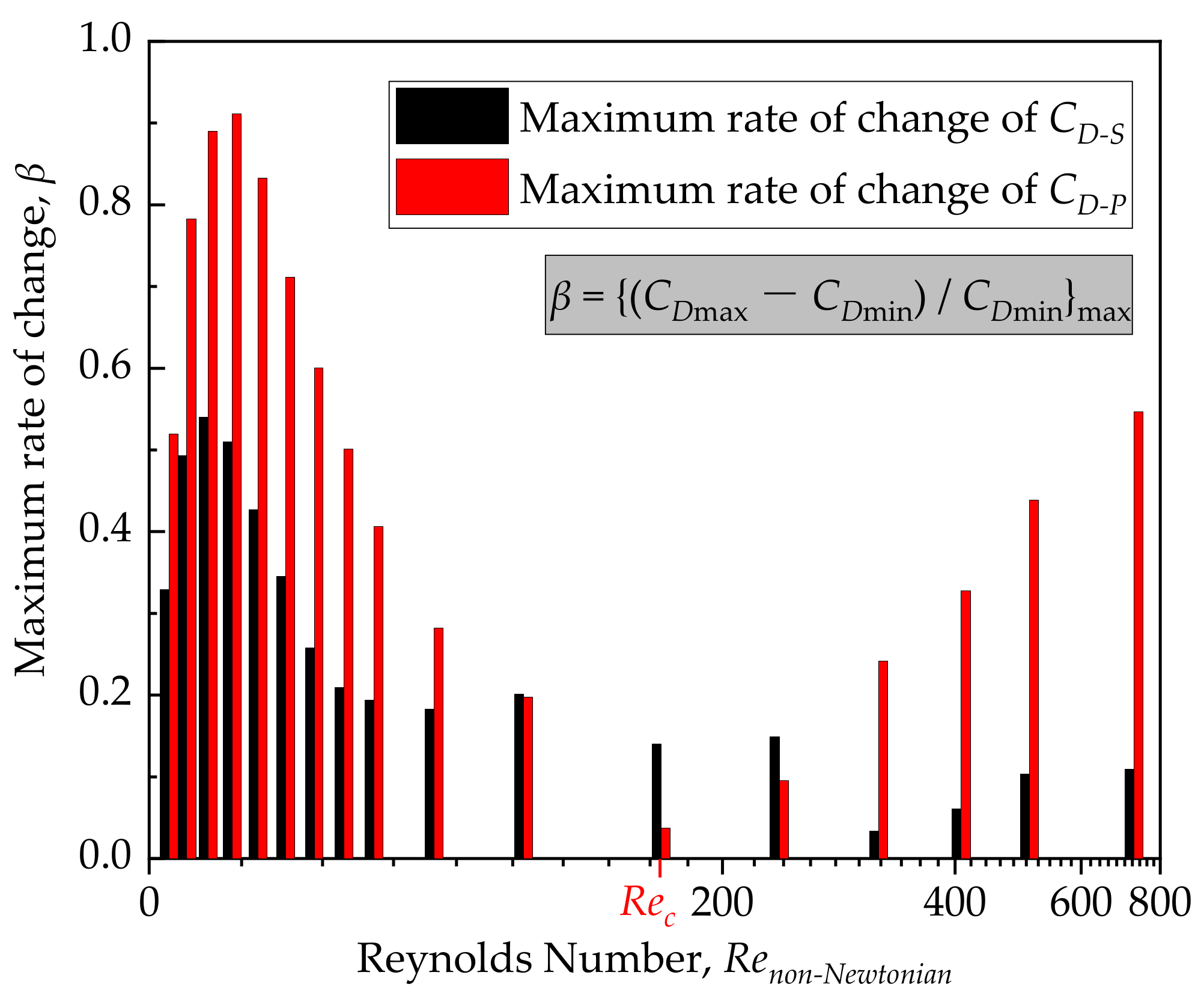
For low Reynolds number (Re_{non-Newtonian} < Re_c), the flow height of the submarine debris flows (H) has a non-negligible influence on C_D, which should be a major consideration in future studies. Moreover, the influence of H on C_D-P and C_D-S is different. The maximum rates of change of C_D-S and C_D-P with respect to different H can reach up to 54% and 91%, respectively.

(4)

The gap between C_D-P and C_D-S changes with Re and H. The maximum gap appears at Re_c = 165.5 and H = D in this study. That is, in engineering design, the peak value, which represents the hazard level of the monopile, may also need to be considered.

The discussion on the interaction force in this study is preliminary, and some issues need to be addressed further. Due to the complexity of the marine geological environment, a simplified interaction model is adopted to estimate the interaction force, which is relatively conservative and limited. Some factors, such as the deformation of the monopile, the interaction between the seabed sediment and the monopile, as well as the applicability of parameters, have not been considered. To obtain a more comprehensive interaction model, additional physical model tests and large-scale simulations need to be performed in the future.

References

1. Randolph, M.; Gourvenec, S. Offshore Geotechnical Engineering; CRC Press: Boca Raton, FL, USA, 2017. [Google Scholar]
2. Bea, R. How sea floor slides affect offshore structures. Oil Gas J. 1971, 69, 88–92. [Google Scholar]
3. Su, C.C.; Tseng, J.Y.; Hsu, H.H.; Chiang, C.S.; Yu, H.S.; Lin, S.; Liu, J.T. Records of submarine natural hazards off SW Taiwan. Geol. Soc. Lond. Spec. Publ. 2012, 361, 41–60. [Google Scholar] [CrossRef]
4. Hance, J.J. Development of a Database and Assessment of Seafloor Slope Stability Based on Published Literature; University of Texas at Austin: Austin, TX, USA, 2003. [Google Scholar]
5. Colella, A.; Prior, D. Coarse-Grained Deltas; John Wiley & Sons: Hoboken, NJ, USA, 2009; Volume 27. [Google Scholar]
6. Silver, M.; Dugan, B. The influence of clay content on submarine slope failure: Insights from laboratory experiments and numerical models. Geol. Soc. Lond. Spec. Publ. 2020, 500, 301–309. [Google Scholar] [CrossRef] [Green Version]
7. Prior, D.; Suhayda, J.; Lu, N.; Bornhold, B.; Keller, G.; Wiseman, W.; Wright, L.; Yang, Z. Storm wave reactivation of a submarine landslide. Nature 1989, 341, 47–50. [Google Scholar] [CrossRef]
8. Zhang, M.; Huang, Y.; Bao, Y. The mechanism of shallow submarine landslides triggered by storm surge. Nat. Hazards 2016, 81, 1373–1383. [Google Scholar] [CrossRef]
9. Coleman, J.M.; Prior, D.B.; Garrison, L.E. Submarine landslides in the Mississippi River delta. In Proceedings of the Offshore Technology Conference, Houston, TX, USA, 7–10 May 1978. [Google Scholar]
10. Norem, H.; Locat, J.; Schieldrop, B. An approach to the physics and the modeling of submarine flowslides. Mar. Georesour. Geotechnol. 1990, 9, 93–111. [Google Scholar] [CrossRef]
11. Zeng, J.; Lowe, D.R.; Prior, D.B.; Wiseman, W.J., Jr.; Bornhold, B.D. Flow properties of turbidity currents in Bute Inlet, British Columbia. Sedimentology 1991, 38, 975–996. [Google Scholar] [CrossRef]
12. Dong, Y. Runout of Submarine Landslides and Their Impact on Subsea Infrastructure Using Material Point Method. Ph.D. Thesis, The University of Western Australia, Perth, WA, Australia, 2017. [Google Scholar]
13. Dengler, A.; Wilde, P.; Noda, E.; Normark, W. Turbidity currents generated by Hurricane Iwa. Geo Mar. Lett. 1984, 4, 5–11. [Google Scholar] [CrossRef]
14. Cornforth, D.H.; Lowell, J.A. The 1994 submarine slope failure at Skagway, Alaska. In Proceedings of the Landslides, Trondheim, Norway, 17 June 1996; pp. 527–532. [Google Scholar]
15. Nodine, M.C.; Gilbert, R.B.; Kiureghian, S.G.W.; Cheon, J.Y.; Wrzyszczynski, M.; Coyne, M.; Ward, E. Impact of hurricane-induced mudslides on pipelines. In Proceedings of the Offshore Technology Conference, Houston, TX, USA, 30 April–3 May 2007. [Google Scholar]
16. Bea, R.G.; Wright, S.G.; Sircar, P.; Niedoroda, A.W. Wave-induced slides in south pass block 70, Mississippi Delta. J. Geotech. Eng. 1983, 109, 619–644. [Google Scholar] [CrossRef]
17. Dou, J.; Chen, J.; Zhang, Z.-J. Influence of large-diameter pipe pile driving on surrounding marine soils and adjacent submarine pipelines. Mar. Georesour. Geotechnol. 2021, 39, 15–33. [Google Scholar] [CrossRef]
18. Zhang, Q.; Zhou, X.L.; Wang, J.H.; Guo, J.J. Wave-induced seabed response around an offshore pile foundation platform. Ocean Eng. 2017, 130, 567–582. [Google Scholar] [CrossRef]
19. Brückl, E.; Scheidegger, A.E. Application of the theory of plasticity to slow mud flows. Geotechnique 1973, 23, 101–107. [Google Scholar] [CrossRef]
20. Zakeri, A. Review of state-of-the-art: Drag forces on submarine pipelines and piles caused by landslide or debris flow impact. J. Offshore Mech. Arct. Eng. 2009, 131, 014001. [Google Scholar] [CrossRef]
21. Zakeri, A.; Høeg, K.; Nadim, F. Submarine debris flow impact on pipelines—Part I: Experimental investigation. Coast. Eng. 2008, 55, 1209–1218. [Google Scholar] [CrossRef]
22. Zakeri, A.; Høeg, K.; Nadim, F. Submarine debris flow impact on pipelines—Part II: Numerical analysis. Coast. Eng. 2009, 56, 1–10. [Google Scholar] [CrossRef]
23. Liu, J.; Tian, J.; Yi, P. Impact forces of submarine landslides on offshore pipelines. Ocean Eng. 2015, 95, 116–127. [Google Scholar] [CrossRef]
24. Zakeri, A. Submarine debris flow impact on suspended (free-span) pipelines: Normal and longitudinal drag forces. Ocean Eng. 2009, 36, 489–499. [Google Scholar] [CrossRef]
25. Wang, Z.; Zhang, Y.; Yu, L.; Yang, Q. Centrifuge modelling of active pipeline-soil loading under different impact angle in soft clay. Appl. Ocean Res. 2020, 98, 102129. [Google Scholar] [CrossRef]
26. Fan, N.; Fauzan, S.; Zhang, W.C.; Nian, T.K.; Randolph, M. Effect of pipeline-seabed gaps on the vertical forces of a pipeline induced by submarine slide impact. Ocean Eng. 2021, 221, 108506. [Google Scholar] [CrossRef]
27. Guo, X.S.; Zheng, D.F.; Nian, T.K.; Yin, P. Effect of different span heights on the pipeline impact forces induced by deep-sea landslides. Appl. Ocean Res. 2019, 87, 38–46. [Google Scholar] [CrossRef]
28. Zhang, Y.; Wang, Z.; Yang, Q.; Wang, H. Numerical analysis of the impact forces exerted by submarine landslides on pipelines. Appl. Ocean Res. 2019, 92, 101936. [Google Scholar] [CrossRef]
29. Guo, X.S.; Nian, T.K.; Wang, Z.T.; Zhao, W.; Fan, N.; Jiao, H.B. Low-temperature rheological behavior of submarine mudflows. J. Waterw. Port Coast. Ocean Eng. 2020, 146, 04019043. [Google Scholar] [CrossRef]
30. Fan, N.; Nian, T.K.; Jiao, H.B.; Jia, Y.G. Interaction between submarine landslides and suspended pipelines with a streamlined contour. Mar. Georesour. Geotechnol. 2018, 36, 652–662. [Google Scholar] [CrossRef]
31. Guo, X.S.; Nian, T.K.; Fan, N.; Jia, Y.G. Optimization design of a honeycomb-hole submarine pipeline under a hydrodynamic landslide impact. Mar. Georesour. Geotechnol. 2020, 1–16. [Google Scholar] [CrossRef]
32. Perez-Gruszkiewicz, S.E. Reducing underwater-slide impact forces on pipelines by streamlining. J. Waterw. Port Coast. Ocean Eng. 2012, 138, 142–148. [Google Scholar] [CrossRef]
33. Dutta, S.; Hawlader, B. Pipeline–soil–water interaction modelling for submarine landslide impact on suspended offshore pipelines. Géotechnique 2019, 69, 29–41. [Google Scholar] [CrossRef]
34. Dong, Y.; Wang, D.; Randolph, M. Quantification of impact forces on fixed mudmats from submarine landslides using the material point method. Appl. Ocean Res. 2020, 102, 102227. [Google Scholar] [CrossRef]
35. Dong, Y.; Wang, D.; Randolph, M. Investigation of impact forces on pipeline by submarine landslide using material point method. Ocean Eng. 2017, 146, 21–28. [Google Scholar] [CrossRef]
36. Qian, X.; Xu, J.; Bai, Y.; Das, H.S. Formation and estimation of peak impact force on suspended pipelines due to submarine debris flow. Ocean Eng. 2020, 195, 106695. [Google Scholar] [CrossRef]
37. Sahdi, F.; Gaudin, C.; Tom, J.G.; Tong, F. Mechanisms of soil flow during submarine slide-pipe impact. Ocean Eng. 2019, 186, 106079. [Google Scholar] [CrossRef]
38. Feng, B.; Sun, H.L.; Qiang, C.Y.; Dong, P.X.; Li, S. Experimental study of submarine landslide impact on offshore wind power piles. Ocean Eng. 2019, 37, 114–121. (In Chinese) [Google Scholar]
39. Elverhoi, A.; Breien, H.; De Blasio, F.V.; Harbitz, C.B.; Pagliardi, M. Submarine landslides and the importance of the initial sediment composition for run-out length and final deposit. Ocean Dyn. 2010, 60, 1027–1046. [Google Scholar] [CrossRef] [Green Version]
40. White, F.M.; Corfield, I. Viscous Fluid Flow; McGraw-Hill: New York, NY, USA, 2006; Volume 3. [Google Scholar]
41. Dey, R.; Hawlader, B.; Phillips, R.; Soga, K. Modeling of large-deformation behaviour of marine sensitive clays and its application to submarine slope stability analysis. Can. Geotech. J. 2016, 53, 1138–1155. [Google Scholar] [CrossRef] [Green Version]
42. Wang, D.; Randolph, M.; White, D. A dynamic large deformation finite element method based on mesh regeneration. Comput. Geotech. 2013, 54, 192–201. [Google Scholar] [CrossRef]
43. Shi, C.; An, Y.; Wu, Q.; Liu, Q.; Cao, Z. Numerical simulation of landslide-generated waves using a soil–water coupling smoothed particle hydrodynamics model. Adv. Water Resour. 2016, 92, 130–141. [Google Scholar] [CrossRef] [Green Version]
44. Pastor, M.; Blanc, T.; Haddad, B.; Petrone, S.; Morles, M.S.; Drempetic, V.; Issler, D.; Crosta, G.; Cascini, L.; Sorbino, G. Application of a SPH depth-integrated model to landslide run-out analysis. Landslides 2014, 11, 793–812. [Google Scholar] [CrossRef] [Green Version]
45. Jiang, M.; Sun, C.; Crosta, G.B.; Zhang, W. A study of submarine steep slope failures triggered by thermal dissociation of methane hydrates using a coupled CFD-DEM approach. Eng. Geol. 2015, 190, 1–16. [Google Scholar] [CrossRef]
46. Si, P.; Shi, H.; Yu, X. A general numerical model for surface waves generated by granular material intruding into a water body. Coast. Eng. 2018, 142, 42–51. [Google Scholar] [CrossRef]
47. Lee, C.H.; Huang, Z. Multi-phase flow simulation of impulsive waves generated by a sub-aerial granular landslide on an erodible slope. Landslides 2021, 18, 881–895. [Google Scholar] [CrossRef]
48. Ma, G.; Kirby, J.T.; Shi, F. Numerical simulation of tsunami waves generated by deformable submarine landslides. Ocean Model. 2013, 69, 146–165. [Google Scholar] [CrossRef]
49. Zhang, Y.; Lu, X.; Zhang, X.; Li, P. Numerical simulation on flow characteristics of large-scale submarine mudflow. Appl. Ocean Res. 2021, 108, 102524. [Google Scholar] [CrossRef]
50. Romano, A.; Lara, J.; Barajas, G.; Di Paolo, B.; Bellotti, G.; Di Risio, M.; Losada, I.; De Girolamo, P. Tsunamis Generated by Submerged Landslides: Numerical Analysis of the Near-Field Wave Characteristics. J. Geophys. Res. Ocean. 2020, 125, e2020JC016157. [Google Scholar] [CrossRef]
51. Zakeri, A.; Hawlader, B. Drag forces caused by submarine glide block or out-runner block impact on suspended (free-span) pipelines—Numerical analysis. Ocean Eng. 2013, 67, 89–99. [Google Scholar] [CrossRef]
52. Ansys, I. ANSYS Fluent Theory Guide; Ansys. Inc.: Canonsburg, PA, USA, 2020. [Google Scholar]
53. Guo, X.S.; Nian, T.K.; Zheng, D.F.; Yin, P. A methodology for designing test models of the impact of submarine debris flows on pipelines based on Reynolds criterion. Ocean Eng. 2018, 166, 226–231. [Google Scholar] [CrossRef]
54. Elger, D.F.; LeBret, B.A.; Crowe, C.T.; Roberson, J.A. Engineering Fluid Mechanics; John Wiley & Sons: Hoboken, NJ, USA, 2020. [Google Scholar]
Figure 1. Interaction forces between submarine debris flows and a monopile. (a) Side view; (b) Top view.
Jmse 09 00736 g001
Figure 2. Geometric model and boundary settings. (a) Top view; (b) side view; (c) aerial view.
Jmse 09 00736 g002
Figure 3. The mesh of the model.
Jmse 09 00736 g003
Figure 4. Mesh sensitivity analysis results.
Jmse 09 00736 g004
Figure 5. Comparison between current calculations and previous experimental results.
Jmse 09 00736 g005
Figure 6. Typical drag force-time curves. (a) High velocity condition; (b) low velocity condition.
Jmse 09 00736 g006
Figure 7. Submarine landslide volume fraction and pressure distribution cloud mapping. (a) Point B1 in model 1. (b) Point C1 in model 1. (c) Point D1 in model 1. (d) Point B2 in model 2. (e) Point C2 in model 2.
Jmse 09 00736 g007
Figure 8. Relationship between CD and Renon-Newtonian at different H. (a) The peak value; and (b) the stable value.
Jmse 09 00736 g008
Figure 9. Relationship between CD and H/D considering different Renon-Newtonian (U). (a) Peak drag force coefficient; and (b) stable drag force coefficient.
Jmse 09 00736 g009
Figure 10. Volume fraction and pressure distribution diagram of submarine debris flow under different flow heights (H) conditions at the peak moment. (a) U = 1.75 m/s, H = D; (b) U = 1.75 m/s, H = 5D; and (c) U = 1.75 m/s, H = 9D.
Jmse 09 00736 g010
Figure 11. Relationship between the maximum drag force coefficient rate of change (β) and Renon-Newtonian considering different H.
Jmse 09 00736 g011
Figure 12. Relationship between residual of drag force coefficient (R) and Renon-Newtonian.
Jmse 09 00736 g012