Article

An Approach to Determine Optimal Bow Configuration of Polar Ships under Combined Ice and Calm-Water Conditions

1
College of Shipbuilding Engineering, Harbin Engineering University, Harbin 150001, China
2
Department of Mechanical and Structural Engineering and Materials Science, University of Stavanger, NO-4036 Stavanger, Norway
3
School of Naval Architecture and Ocean Engineering, Jiangsu University of Science and Technology, Zhenjiang 212003, China
*
Author to whom correspondence should be addressed.
J. Mar. Sci. Eng. 2021, 9(6), 680; https://doi.org/10.3390/jmse9060680
Submission received: 9 June 2021 / Accepted: 17 June 2021 / Published: 21 June 2021
(This article belongs to the Special Issue Ship Dynamics and Hydrodynamics)

Abstract

:
Selecting an optimal bow configuration is critical to the preliminary design of polar ships. This paper proposes an approach to determine the optimal bow of polar ships based on present numerical simulation and available published experimental studies. Unlike conventional methods, the present approach integrates both ice resistance and calm-water resistance with the navigating time. A numerical simulation method of an icebreaking vessel going straight ahead in level ice is developed using SPH (smoothed particle hydrodynamics) numerical technique of LS-DYNA. The present numerical results for the ice resistance in level ice are in satisfactory agreement with the available published experimental data. The bow configurations with superior icebreaking capability are obtained by analyzing the sensitivities due to the buttock angle γ, the frame angle β and the waterline angle α. The calm-water resistance is calculated using FVM (finite volume method). Finally, an overall resistance index devised from the ship resistance in ice/water weighted by their corresponding weighted navigation time is proposed. The present approach can be used for evaluating the integrated resistance performance of the polar ships operating in both a water route and ice route.

1. Introduction

The bow configuration of a polar ship is determined by a basic idea, i.e., the minimum power to move forward in the ice. From the design point of view, level ice resistance is also one of the most significant factors. There are many cases of polar ships with self-icebreaking ability sailing in level ice, for example, PUGNAX (polar deck carrier) [1], MV Xue Long (polar scientific research vessel) and MV Xue Long II. At the current stage of polar exploration, this kind of ship sailing in level ice is also considered as an important condition. The primary requirement for these polar ships is a good performance in level ice. Good performance means low ice resistance, high propulsive efficiency and guaranteed continuity in icebreaking [2]. Some researches [3,4,5] suggested that ice resistance is the main contribution to the total resistance in level ice. Apart from the ice properties and the power of polar ships, the ice resistance is significantly influenced by the bow configurations. In the evolution of the bow configuration, the frame angle has been increasing, while the waterline angle has decreased, and the buttock angle has reduced from about 30° to 20° in the early years [6]. From the perspective of ship–ice interaction, a description about the changes of the bow angles is explained below. When the ship is operating in ice region, the ice is crushed at the stem post of the bow. The buttock angle has been reduced because a smaller buttock angle induces more bending moment and less horizontal force. The waterline angle mainly affects the crushed ice-pushing capability of the bow. The decrease in waterline angle leads to the decrease in longitudinal crushed ice force. However, the bow needs more contact area and extrusion force to bend the ice with the decrease in frame angle. Therefore, the purpose of these changes of the bow angles is to achieve a superior icebreaking capability of a polar ship. It seems that the bow configurations of modern polar ships are quite similar. The ice resistance may nevertheless show notable differences. Consequently, all the changes of the bow configuration aim to obtain a superior icebreaking capability of polar ships navigating in ice region.
Several methods for ice resistance prediction have been proposed, which take into account the influence of geometric variations of the hull. In practical ship design, empirical or semi-empirical prediction methods may be applied to estimate the resistance in the preliminary design phase. Erceg and Ehlers [7] reviewed six semi-empirical level ice resistance prediction methods (Vance [8]; Lewis et al. [9]; Zahn and Phillips [10]; Keinonen [11,12]; Lindqvist [13]; Riska et al. [14]). Ice resistances of four ships with different sizes were calculated and compared based on the six semi-empirical prediction methods. The methods show significant discrepancies for larger ships, with differences in the predicted ice resistance as large as 100–200%. In the study of Lindström [15], most of the relevant ice parameters and hull configurations including the bow angles were regarded in the ice resistance prediction. Based on the study of Lindqvist [13], Riska et al. [14] proposed a formula for calculating the level ice resistance. This formula takes into account the particulars of the ship and the ice thickness. The empirical coefficients are derived from full-scale tests performed in the Baltic Sea. Jeong [16] decomposed the ice resistance into ice buoyancy resistance, ice-clearing resistance and icebreaking resistance. Using the component method, Jeong [16] conducted an ice model test of MOERI standard icebreaker model, and non-dimensional coefficients in ice resistance prediction formula are obtained based on the data of model test. Lubbad and Løset [17] established new analytical closed-form solutions to represent the icebreaking process of ship–ice interaction in real-time. These works have offered good insights into the method of estimating the ship performance accounting for ship–ice interaction.
Because the experimental research can reveal real physical effects of ship–ice interaction, some detailed analyses have been carried out to study the bow configurations based on the full-scale experiment as well as the ice model tests. Varges [18] investigated the bow shape of an icebreaker based on the full-scale experiment. The vessel of concern was the Soviet polar icebreaker MUDYUG, which was built in 1972 and given a new Thyssen/Waas forebody in 1986. The conventional angled bow was replaced with a form more resembling a sled. The sleigh-shaped bow has better performance and less vibration in the icebreaking process. Based on the ice model test results of HSVA’s database from 1996 to 2014, Myland and Ehlers [19] focused in particular on the icebreaking patterns in level ice with regard to relevant hull shape parameters. The ship models with similar scales were chosen for analysis, so as to have model ice conditions, model speed values and ship model dimensions in the same range.
More recently, numerical simulations, e.g., discrete element method (DEM) and finite element method (FEM), have been widely used to analyze the influence of ship hull forms on the ice performance. Lu et al. [20] applied FEM to calculate the ice load acting on conical structures colliding with level ice. The mesh size dependency of the bending failure of level ice was eliminated by taking into account the random spatial distribution of material properties. Wang and Zou [21] used FEM to investigate the effects of the wedge stem and the shovel stem on the damage of the ice layer and the resistance during the icebreaking process. The result of wedge-shaped bow and scoop bow in the process of icebreaking were compared, and some suggestions for the design of icebreaker hull lines were given. Li et al. [22] estimated the ice load acting on the shoulder and midship of a polar ship by applying the extended finite element method (XFEM). Long et al. [23] adopted DEM with the bond and failure model to simulate the breaking process of sea ice colliding with a conical structure and vertical pile. The results showed that the bending failure occurs as the ice cover moves upward or downward, depending on the water level. Wang et al. [24] combined an elastoplastic softening constitutive model with cohesive element method (CEM) to simulate the continuous icebreaking process in level ice. This method captured well the main features, including the local crushing and the bending failure, of the ship–ice interactions.
In the past few years, the smoothed particle hydrodynamics (SPH) method has been used to effectively model large deformation and failure behavior of solids, including ice. Das and Ehlers [25] carried out a numerical simulation of crushing and bending failure of ice using SPH. In their study, the numerical bending results for force, displacement and failure time were compared with earlier simulations of in situ four-point bending test results and finite element simulations. The crushing failure was compared with experiments conducted by Häusler [26], and it was found that the SPH approach was in good agreement with the experiment. Furthermore, the SPH method is extended so as to simulate the actual behavior of sea ice as ships progress through level ice. Zhang et al. [27] reported that the SPH results agreed well with the experimental data of three-point bending test. This implies that the present SPH model can produce accurate results for simulating the ice failure problem. Zhang et al. [27] also showed a good agreement between the results of the SPH and the experimental data for the ice–ship interaction. They indicated that the numerical accuracy and stability of SPH were satisfactory.
Usually, polar ships also navigate in water ways, but the calm-water performance is ignored in the researches above. Especially for polar ships converted from the merchant vessel, which, most of the time, are operated in both water ways and ice regions. It is necessary to conduct integrated analyses that account for the resistance both in ice and in water. However, the literature on the optimization of bow configuration of polar ships navigating in combined routes is limited. Polach et al. [28] proposed a method which includes the ship performance evaluation based on ship merit factor (SMF). This method combined SMF with a route-specific ship and allows one to compare the technical and economic performance of ships operating in open water and ice. The performance of different ship designs that operated along the route Rotterdam to Yokohama through the Suez Canal and the Northern Sea Route was studied.
This study aims at devising an approach to determine the optimal bow of polar ships operating in both water route and ice route. In the paper, a numerical simulation of an icebreaking vessel going straight ahead in level ice is performed using the SPH numerical technique. The present numerical results are compared with the experimental data by Zhou et al. [29]. A polar research vessel, MV Xue Long, is used as a reference ship to demonstrate the usage of the proposed approach. Comparative analyses are carried out to evaluate the sensitivities of the buttock angle γ, the frame angle β and the waterline angle α on the icebreaking capability. Integrated numerical simulations are conducted to study the icebreaking capability and calm-water performance of the polar ship with different bow configurations. An overall resistance index Cr is proposed to determine the optimal bow configuration of polar ships navigating in a combined route.

2. Validation of Ice Material Model

According to the mechanical properties of ice, the constitutive model of ice is established using the SPH method. The numerical model is validated by comparing the results with the experiment by Kim et al. [30]. Furthermore, a ship–ice–water interaction model is proposed for the simulation of a ship moving in level ice. The present numerical results for the icebreaking patterns and the ice resistance are then compared with the experimental data by Zhou et al. [29].

2.1. Verification of Ice Material Model

During the process of deformation to failure of ice, the ductile–brittle transition occurs due to the effect of the loading rate. The behavior of ice at high strain rates (greater than 10−3 s−1) is similar to the linear elastic material with brittle failure [31]. The material model takes into account high strain rates and is widely used to model the dynamic behavior of ice including elastic deformation and brittle fracture. Strain rate (s−1) is the change in strain of a material with respect to time. In this study, the strain rate effect was transformed to the strain effect included in the material model. An isotropic elastic-plastic material model with a von Mises yield surface was used in the numerical simulation.
The von Mises yield condition is given by:
ϕ = J 2 σ y 2 3
where the second stress invariant, J2, is defined in terms of the deviatoric stress components as
J 2 = 1 2 s i j s i j
and the yield stress, σ y , is a function of the effective plastic strain, ε e f f p , and the plastic hardening modulus, Ep:
σ y = σ 0 + E p ε e f f p
Pressure is given by the expression
p n + 1 = K ( 1 V n + 1 1 )
where n is the number of time steps, K is the bulk modulus, and V is the relative volume defined as the ratio of the current volume over the initial volume.
When an element reaches the plasticity phase under the action of compression, it follows the yield surface until failure. An element is removed by erosion if the pressure surpasses the failure pressure. Meanwhile, failure by element erosion is activated if the equivalent plastic strain reaches the plastic failure strain. The values including plastic failure strain and failure pressure for the cone-shaped ice were also used in the ice sheet simulations. When the ice breaks, compression failure acquirement is met, as shown in Table 1.
In order to verify the accuracy of the above constitutive model of ice, a numerical simulation was carried out on the compressive cone-shaped ice experiments [30]. The models of cone-shaped ice and steel plate for the present numerical simulation are shown in Figure 1a. The SPH method is used to simulate the cone-shaped ice with a diameter of 100 mm and a cone angle of 120 degrees. In the bottom plane of the numerical cone-shaped ice, the movement of SPH particles is constrained to six degrees of freedom to simulate the ice fixed on the experimental device. A rigid body is used to simulate the steel plate. The cone-shaped ice is vertically compressed by the steel plate at the speed of 1 mm/s and 100 mm/s. The brittle fracture was observed in the numerical calculations, as shown in Figure 1b,c.
Figure 2a gives the convergence tests on compression force, in which N is the total particle number. Three particle numbers of 27,974; 37,196 and 51,192 are tested in the compressive cone-shaped ice. The relative error Erf is defined as the errors between experimental results [30] and SPH results, which are calculated by:
E r f = i = 1 n ( f i f 0 i ) 2 / i = 1 n f 0 i 2
where fi is the compression force of SPH with different particle numbers at t = ti; and f0 is the compression force of experimental data at t = ti. The results of Figure 2a indicate that the errors of the compression force decrease with the increasing particle number and demonstrate a roughly first-order convergence ratio. Therefore, 37,196 particles are deemed adequate for the simulation of ice cone. The force-displacement curves of the numerical simulation at the compression speed of 1 mm/s and 100 mm/s are presented in Figure 2b,c. Numerical results are compared with the experimental data [30]. It is found that, in both the high-speed loading and the low-speed loading, the ice force increases with the displacement. As shown in Figure 2b,c, the force pattern is captured by the numerical simulation with satisfactory accuracy. The numerical method agrees better with the experiment in the amplitude of ice force for lower loading speeds. It also can be seen that more fluctuations are present in the solution for higher loading speed. When the ice is broken to a certain length, the ice force does not increase but decrease due to the unloading of the pressure. In Figure 2b,c, the strain rate is 10−2 s−1 for v = 1 mm/s, and 1 s−1 for v = 100 mm/s. Both fall into the range of high strain rates (>10−3 s−1), where the ice has the behavior as brittle materials. Moreover, the same cut-off stress value is used in the present numerical ice model. In fact, the cut-off stress decreases slightly with the increase in loading speed in the brittle range. This is why the peak contact forces are somewhat close (35 and 38 kN, respectively), and the present numerical method shows a little overestimation of the amplitude for a higher loading speed. The comparisons show that the present numerical ice model can give a similar trend of the compression process of ice with that of the experiment, although there are some differences in details.

2.2. Description of Model Test

Zhou et al. [29] conducted a series of ice resistance tests where the model of an icebreaking vessel, MT Uikku, was towed in an ice basin. A scale model of 1:31.6 was built without any appendices such as rudders and propellers. The full-scale primary dimensions of MT Uikku are given in Table 2. The model was towed with the carriage to simulate the ice–hull interaction process. In the model tests, the ice drift angle and the hull heading angle were constant at 0°. The ice force was measured and digitally sampled on a computer and recorded as an analogue signal as a back-up. The measured data were sampled at a frequency of 107 Hz. The test program and measured ice properties are summarized in Table 3, where hi is ice thickness; σb and σc are bending strength and compressive strength of ice; Ei is the elastic modulus of ice; and Vi is ship speed.

2.3. Numerical Simulation

A finite element ship model of the MT Uikku is created in the numerical simulation. The ship form parameters are presented in Table 2. The icebreaking pattern and the ice resistance are investigated regardless of the response of ship structures. Therefore, only the hull of the ship is established and simplified to a rigid body in the present numerical simulation. The model is going straight ahead in the x-direction at predefined constant speeds. Based on the SPH numerical technique of LS-DYNA hydrocode, the problem of a ship moving in level ice is simulated. The dimensions of domain are 600 m × 150 m × 75 m. The level ice floats on water, and its two long sides are constrained in the x-direction.
In the mathematical description of fluid, the equation of state describes the relationship between volume deformation and pressure. The null material is used to describe the water flow. The Gruneisen equation is adopted to describe the state of water. The parameters used in the numerical simulation are shown in Table 1. The force data are sampled every 0.01 s. Figure 3 shows the typical configuration of the numerical model applied to calculate the ice resistance.

2.4. Comparisons and Discussions of Results

Numerical simulations are performed to simulate the Test 1 and Test 2 in Table 3. Figure 4 shows the icebreaking stress and the icebreaking pattern in the numerical simulation of Test 2. As shown in Figure 4a, the stress is generated by the deformation of the ice, which mainly occurs in the contact area between ice and hull. A concentrated area of high stress is present near the bow, and larger ice pieces are observed in the bow and shoulder area. As the hull goes straight ahead in level ice, the open channel is generated in Figure 4b. As can be seen in Figure 4a,b, the width of the channel is approximately equal to the beam of the model ship. The icebreaking patterns obtained in the present numerical simulation is similar to that in Zhou et al. [29].
Figure 5a gives the convergence tests on ice resistance, in which M is the total particle number. Three particle numbers of 210,555; 262,709 and 307,601 are tested in the icebreaking simulations. The relative error Err is defined as the errors between experimental results [29] and SPH results, which are calculated by:
E r r = | r 0 r | / r 0
where r is the ice resistance of SPH with different particle numbers from t = 0 s to t = 30 s, r0 is the ice resistance of experimental data from t = 0 s to t = 30 s. The results of Figure 5a indicate that the errors of the ice resistance decrease with the increasing particle number and demonstrate a roughly first-order convergence ratio. Hence, 262,709 particles are deemed adequate for the simulation of icebreaking. Time histories of ice forces in the longitudinal direction of Test 1 and Test 2 (Table 3) from the present simulation and the experiment [29] are presented in Figure 5b,c. Since the ice resistance commonly refers to the time average of all longitudinal forces due to ice acting on the ship, a comparison of results in a quantitative way is conducted. The mean values of the ice forces at the steady stage are also presented in Figure 5b,c. The differences between numerical results and model test data are identified to a certain extent. The ice force fluctuates during the icebreaking process while the force is never zero. This is because that there are always multiple ice contacts along the hull as the ship moves forward. These contacts are a series of events during the process, and the ice forces are the summation of all the contact forces. In addition, ice submergence resistance is a significant contribution. Some previous numerical simulation, e.g., [3], shows that submersion plays a significant role even at slow speed. The existence of submersion is also one of the reasons that the time history of ice forces rarely drops to zero. The mean values of the present simulation results for the ice forces, i.e., ice resistance, approach those of the experimental data from [29]. The fluctuation amplitudes of the simulated ice force are slightly higher than those of the experimental results. Figure 4b shows that the pieces of large ice cusps generated in the present numerical simulation are more than those observed in the experiment [29]. Data processing methods in Wang et al. [24] are referenced in Figure 5b,c. In order to eliminate the noise from the results, the numerical force curves are plotted by processing the original data through the filter used in the experiment. Higher fluctuation amplitudes of calculated ice resistance have been reduced. The results of the present numerical simulations are in better agreement with the experimental data. The ice resistances of numerical simulations and experiments are denoted by Ri num and Ri exp in Table 4, respectively. The standard deviations (StDev) of Ri num are 156 kN for Test 1 and 99 kN for Test 2. The standard deviations of ice resistance versus the mean value (CV) for Ri num are 0.31 for Test 1 and 0.16 for Test 2. The relative errors (Er) between Ri num and Ri exp are 9.04% for Test 1 and 10.56% for Test 2. Although this observation indicates that the present numerical simulation cannot capture all the details of the broken ice floes around the hull, the approach adopted here, as shown in the comparative analyses above, is appropriate for evaluating the ice resistance performance. Thus, the present approach can serve as a tool to study the bow configuration of the polar ship.

3. Approach to Determine the Optimal Bow Configuration of Polar Ships

Based on the dimensions of MV Xue Long, a full-scale hull model is established. The full-scale model is taken as the master model. Nine hull models are created with different bow configurations so as to analyze the icebreaking capability. Then, the models are moved in the calm water (without ice) at a speed of 15 knots. The workflow of the approach is shown in Figure 6.

3.1. Ship Model and Bow Configuration Parameters

An icebreaking scientific research vessel, MV Xue Long, is modeled for the present study. MV Xue Long is an icebreaking research vessel owned by the Polar Research Institute of China. It was built at the Kherson Shipyard in Ukraine in 1993. It started as an icebreaking cargo and supply ship designed for the Russian Arctic. It was then converted from an Arctic cargo ship to a polar research and resupplying vessel by the mid-1990s. The ice class of MV Xue Long, assigned by the China Classification Society (CCS), is B1 [32].
The primary dimensions of MV Xue Long are presented in Table 5. As the present study focuses on the bow configuration instead of the structural response, the ship is modeled as a rigid body without any hull structures. The finite element model of the hull is shown in Figure 7. The bow configuration can be characterized by the buttock angle γ, the frame angle β and the waterline angle α [33], as illustrated in Figure 8.

3.2. Schemes of Bow Configuration

An analysis is conducted to analyze the effect of γ on the icebreaking capability, which is done by varying γ with α and β being fixed. In the simulations, the ship model is going straight ahead in level ice (hice = 0.5 m). The speed the ship can attain in level ice is calculated based on the present numerical simulation. The ice resistance equals the extra thrust available at different power levels and speeds. The net thrust curves used in the analysis are based on the theoretical calculation given by Equation (7) [34] and are considered as a preliminary curve. The average longitudinal speed the ship achieves in the designated ice conditions is determined from the intersection of the net thrust curve and the ice resistance curve.
T n e t = T B [ 1 1 3 u v o w 2 3 ( u v o w ) 2 ]
where TB is the bollard pull; u is the initial ship speed; and vow is the maximum calm-water speed.
Figure 9a shows the effect of γ on the average longitudinal ship speed. It can be seen that the relationship between the longitudinal ship speed in the continuous icebreaking process and γ is approximately a downward curve. The main reason is that a small γ induces a large bending moment and a small horizontal force. The effects of α and β on the average longitudinal ship speed are also analyzed using in the same manner. Figure 9b shows the average longitudinal ship speed for α = 17°, 21°, 25°, 29° and 33° with γ fixed to 23° and β to 53°. It is observed that the longitudinal ship speed decreases slightly with α increases. The reason is that the longitudinal crushed ice force Fx increases with α and results in the decrease in the longitudinal ship speed, as shown in Figure 9d. Unlike γ and α, β has a non-monotonic effect on the longitudinal ship speed when γ is fixed to 23° and α to 25°, as shown in Figure 9c. A fluctuating pattern of the influence of β on the average longitudinal speed is observed. However, the difference between the maximum and the minimum ship speed is less than 4%. It suggests that β has little effect on the total ice resistance and the ship speed.
To determine the optimal bow configuration, schemes of combinations of α, γ and β are obtained using the orthogonal design method [35]. A comprehensive research with three factors (α, γ and β) at three levels (i.e., three values of each factor) requires twenty-seven different cases. By using the orthogonal design method, there are only nine non-repetitive cases. As shown in Figure 10, the nine cases are evenly distributed in the entire research domain. The bow configuration schemes and parameters used in the orthogonal design are listed in Table 6.

3.3. Sensitivity of the Icebreaking Capability to the Bow Configuration Parameters

Sensitivity studies are carried out to analyze the influence of bow configurations on the icebreaking capability. Analysis of variance is employed to identify the critical affecting factor in the significance tests. The variance of the test results originates from the test errors and the variations of different factors:
S T = Q T P
where ST denotes the total variance of the test results. QT is the sum of squares of the indicators, and P is the revised value.
Q T = k = 1 n x k 2
P = 1 n ( k = 1 n x k ) 2
where n is the total number of tests, and xk is the indicator for each test.
The variance of each factor can be expressed as
S A = Q A P
where
Q A = 1 a i = 1 n a K i 2
K i = j = 1 a x i j
where Ki denotes the sum of test results for factor A at level i. a is the number of tests for each level, and xij is the indicator of j-th test for factor A at level i.
Taking the ice resistance as the indicator of the icebreaking capability, Table 6 presents the variance analysis results for the significance test, where T is the sum of indicators. The variance of factors at three levels are ranked in the order of Sγ, Sβ, and Sα.
The total variance of the test results ST = QT P = 110,800, and the variance of the test error SE = ST   Sα   Sγ   Sβ = 2400. Table 7 shows the significance test results of the effects of α, γ and β on the ice resistance, where d.f. denotes the degrees of freedom. The total d.f. of the test fT = n  1 = 8, the d.f. of each factor fA = na  1 = 2, and the d.f. of the test error fE = fT   fα   fγ   fβ = 2.
F is defined as the mean squared deviation (Mean Sq.) of each factor divided by the mean squared deviation of test error, which represents the magnitude of the sensitivity of each factor to the test results. Here, the F values of α, γ and β are 1.70, 40.5 and 3.01, respectively. Compared with the F-critical value, i.e., F0.05(2, 2) = 19.0, which is obtained by a joint hypotheses test, the F value of γ is greater, indicating that γ has a significant effect on the test results. In other words, γ is the most important factor to the ice resistance, marked with *. In contrast, the F values of α and β are much less than 19.0, suggesting that the effect of α and β on the ice resistance is insignificant. Therefore, the bow configurations from Case 1, Case 4 and Case 7 have an excellent icebreaking capability, which is achieved with the minimum value of γ (i.e., γ = 22°).

3.4. Integrated Evaluation Based on the Resistance Performance

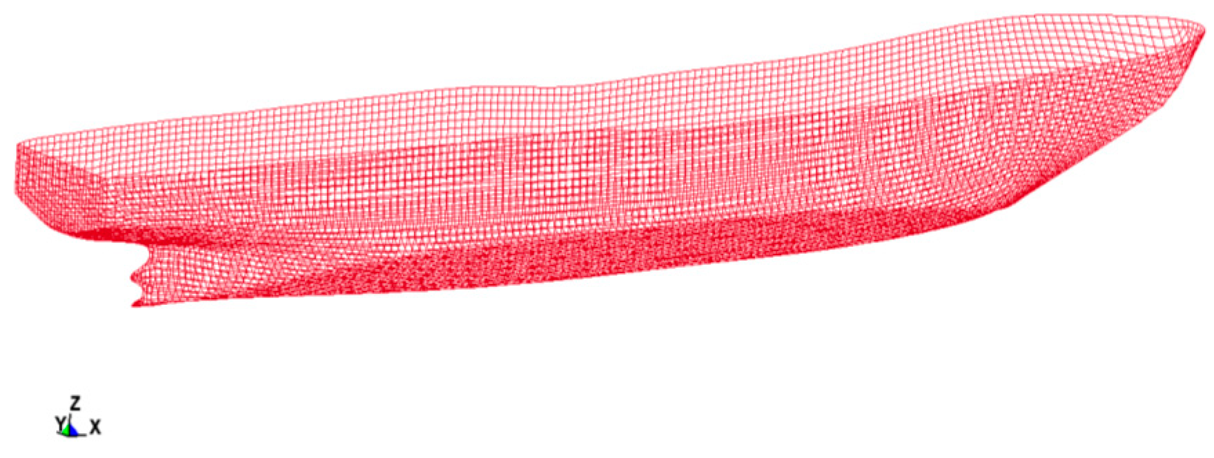
For polar ships sailing in both water and ice regions, it is economically beneficial to consider both water resistance and ice resistance by using a typical route for conceptual design. In the present study, the calm-water resistance of Case 1, Case 4 and Case 7 is calculated using the FVM-based commercial code of STAR-CCM+. The fluid domain and mesh of the present numerical model are shown in Figure 11a. The ship speed is 15 knots for the estimation of calm water resistance, which represents the design speed during operation. A grid convergence study and time-step study are performed in order to verify the present numerical model. Table 8 indicates the grid information and the resulting average calm-water resistance. Three grid numbers of 1,357,071; 3,088,921, and 4,401,879 are tested, respectively. Figure 11b shows the plot of average calm-water resistance with varying grid numbers. As the grid number increases, the average calm-water resistances approach an asymptotic infinite-grid number value. Three simulations (coarse, medium and fine) are completed with a constant refinement ratio r = 2. The order of convergence, p, is calculated using:
p = ln [ ( 193.875 188.520 ) / 188.520 188.385 ] / ln ( 2 ) = 5.31
Richardson extrapolation is performed to predict an estimate of the value of the average calm-water resistance at infinite grid number,
f n = 188.385 + ( 188.385 188.520 ) / ( 2 5.31 1 ) = 188.382 ( kN )
This value is also plotted on Figure 11b. The grid convergence index for the fine grid solution can now be computed. A factor of safety of FS = 1.25 is used since three grids were used to estimate the average calm-water resistance. The grid convergence index (GCI) for the medium and fine refinement levels is:
G C I 23 = 1.25 | ( 188.520 188.385 ) / 188.385 | / ( 2 5.31 1 ) 100 % = 0.002316 %
The grid convergence index (GCI) for the coarse and medium refinement levels is:
G C I 12 = 1.25 | ( 193.875 188.520 ) / 188.520 | / ( 2 5.31 1 ) 100 % = 0.091826 %
Grids are ensured in the asymptotic range of convergence by checking:
0.091826 % / ( 2 5.31 0.002316 % ) = 0.99938
which is approximately one and indicates that the solution is well within the asymptotic range of convergence. Therefore, 3,088,921 grids are sufficient to produce accurate results, which are used to calculate the calm-water resistance.
For the time-step convergence study, the time step is selected based on the numerical simulations in which a variety of Courant numbers, C = 0.075, 0.1, 0.25, and 0.5 are carried out. The Courant number describes the relationship between the time step and the space step. Intuitively speaking, the Courant number is the number of grids that a fluid particle can pass through in a time step. As shown in Figure 11c, when the Courant numbers of 0.075 and 0.1, the calm-water resistance obtained with Courant number being 0.075 and 0.1 is insignificant. Therefore, the Courant number C of 0.1 is used in this present study.
Figure 12 shows the time histories of the calm-water resistance for Case 1, Case 4 and Case 7. The calm-water resistance amplitude in the stable range, from 80 to 200 s, is used to calculate the mean value, i.e., the average calm-water resistance. Comparison of the numerical results shows that Case 7 has the maximum calm-water resistance. As can be seen in Table 6, Case 7 has the fullest bow, corresponding to the largest α and β, resulting in the maximum calm-water resistance. Results for the average calm-water resistance (Rwater) and the ice resistance (Rice) are presented in Table 9. It was found that the average calm-water resistance for Case 4 is about 3.87% larger than Case 1, and the average calm-water resistance for Case 7 is 4.79% larger than Case 4. The ice resistance for Case 4 is 3.35% smaller than for Case 1, and the ice resistance for Case 7 is 8.09% smaller than for Case 4. Rwater and Rice are significantly influenced by the bow configuration. The present results indicate that full bows are favorable for the performance in the ice but not beneficial to the performance in the calm-water. In addition, Table 9 shows that total resistance in the ice region is more than four times higher than in water region, because it is assumed that the ship speed is fixed to 15 knots in the water route and the invariant ice thickness is 0.5 m in the ice region. In this case, the ice resistance is approximately four times higher than the water resistance. However, the speed changes when the ship navigates along the ice routes according to the ice condition, such as the variety of ice thickness. In addition, the ship probably does not sail at the same speed in the water region. Therefore, the ratio of the ice resistance to the water resistance is not constant.
In most ice regions, the ship speed changes when a ship navigates along the ice routes according to the ice condition, such as the variety of ice thickness. If the ship captain wants to achieve a certain speed in the ice region, the ship needs to overcome resistance in ice. For that purpose, propeller must provide sufficient thrust, i.e., the ship engine is selected based on this. Ship probably does not sail at the same speed in ice region and in region without ice due to significantly different total resistances. In this case, the entire route of a polar ship should be divided by different segments based on ship speed from the harbor to the ice region. Thus, an overall resistance index Cr comprising the ship resistance and the corresponding weighted navigation time is proposed as follows,
C r = i = 1 m k w a t e r i R w a t e r i + j = 1 n k i c e j R i c e j
where kwater i and kice j are the weight factors of the i-th route segment in the water region and the j-th route segment in the ice region, respectively; Rwater i and Rice j are the resistance of the i-th route segment in the water region and the j-th route segment in the ice region, correspondingly.
In the present study, Cr is calculated by only one uniform water segment and one uniform ice segment. It is assumed that the speeds of a polar ship in calm water and in level ice are both constant. For MV Xue Long, the weighted factor kwater is assumed to be 0.8, and kice is 0.2. Cr of Case 1, Case 4 and Case 7 is shown in Table 9, where Cr of Case 7 is the smallest. Therefore, Case 7 is selected as the optimal bow configuration for overall performance in both water and ice. It should be noted that kwater and kice are consistent with the actual navigation time of the polar ship of concern. For example, in August 2017, the Russian icebreaking LNG carrier Christophe de Margerie [36] passed through the Northern Sea Route (NSR) in six days and completed the entire 19-day journey from Hammerfest, Norway, to Boryeong, South Korea. In this case, kwater = 0.68 and kice = 0.32 can be used according to the article posted by Rachael [36]. The present method can be used to improve and optimize the bow configuration by assessing the resistance performance. The optimal route of a polar ship from the harbor to the ice region can also be studied using Equation (14). For the operation of vessels in the different routes, the mileage is considered in kwater and kice.

4. Conclusions

An approach to determine the optimal bow of polar ships based on present numerical simulation and available published experimental studies was proposed. In order to validate the constitutive model of ice, numerical simulations were performed using SPH, and the results were compared with the experiment by Kim et al. [21]. Then, a ship–ice–water interaction model was proposed for the simulation of a ship moving in level ice. The present numerical results for the ice resistance in level ice were in satisfactory agreement with the experimental data by Zhou et al. [20]. This method was then used to analyze the ice resistance of a polar ships with various bow configuration parameters, including the buttock angle γ, the frame angle β and the waterline angle α. Sensitivity analyses of the ice resistance to these parameters were evaluated by performing the analysis of variance. It was found that the effect of γ on the ice resistance is much more significant than that of α and β; thus, small γ values are desirable.
To assess the overall resistance performance of a ship that is operated in both ice and waters regions, the resistance in water was calculated using the FVM-based method. Then, an overall resistance index Cr devised from the ship resistance in ice/water weighted by their corresponding weighted navigation time was proposed. The formula to calculate the index takes a simple form but is particularly useful in practice as the resistances and weights can be easily obtained. Since the bow geometry is the most important factor to the overall resistance performance, the proposed formula provides a convenient approach to determine the optimal bow configuration of polar ships. A polar research vessel, MV Xue Long, was used as a reference ship to demonstrate the usage of the proposed formula. In most cases, the entire route of a polar ship should be divided by different segments based on ship speed from the harbor to the ice region. In the present study, Cr was calculated by one uniform water segment and one uniform ice segment. It was assumed that the speeds of a polar ship in calm water and in level ice are both constant. More calculations by Equation (14) are needed when the route is divided by different segments based on ship speed. In addition, the present approach is applied to the evaluation based on the resistance performance of polar ships moving in level ice, which is a typical condition for polar ships with self-icebreaking ability. For merchant polar ships that may be operated in pack ice, improvement and validation of the approach shall be made for the desired accuracy.

Author Contributions

Conceptualization and methodology, H.L., Y.F. and M.C.O.; software, validation and formal analysis, Y.F. and X.Z.; investigation, H.L., Y.F., M.C.O. and L.Z.; resources, H.L., M.C.O. and L.Z.; writing—original draft preparation, H.L. and Y.F.; writing—review and editing, H.L., Y.F., M.C.O., X.Z. and L.Z.; visualization, H.L., Y.F. and X.Z.; supervision, H.L. and M.C.O.; project administration and funding acquisition, H.L. All authors have read and agreed to the published version of the manuscript.

Funding

This research was funded by National Natural Science Foundation of China, grant number 52071110.

Institutional Review Board Statement

Not applicable.

Informed Consent Statement

Not applicable.

Data Availability Statement

Not applicable.

Acknowledgments

The authors would like to acknowledgment College of Shipbuilding Engineering, Harbin Engineering University in purchasing and supporting the use of LS-DYNA and STAR-CCM+ software. The authors would also like to thank X. Q. Zhou in Harbin Engineering University for his discussions and suggestions.

Conflicts of Interest

The authors declare no conflict of interest.

References

  1. van Lievenoogen, R.; Hovilainen, M.; Ville, V. AUDAX and PUGNAX, Unique PC-3 Class Heavy Transport Vessels Designed for Module Transportation for LNG Liquefaction Projects in Arctic Remote Locations. In Proceedings of the OTC Arctic Technology Conference, Houston, TX, USA, 5–7 November 2018. [Google Scholar]
  2. Myland, D.; Ehlers, S. Theoretical investigation on ice resistance prediction methods for ships in level ice. In Proceedings of the 33rd International Conference on Ocean, Offshore and Arctic Engineering, OMAE 2014-23304, San Francisco, CA, USA, 8–13 June 2014. [Google Scholar]
  3. Valanto, P. On the cause and distribution of resistance forces on ship hulls moving in level ice. In Proceedings of the 16th International Conference on Port and Ocean Engineering Conference under Arctic Conditions, POAC’01, Ottawa, ON, Canada, 12–17 August 2001. [Google Scholar]
  4. Puntigliano, F. Experimental and Numerical Research on the Interaction between Ice Floes and a Ship’s Hull during Icebreaking. Ph.D. Dissertation, Technical University Hamburg-Harburg, TUHH, Hamburg, Germany, 2003. [Google Scholar]
  5. Riska, K. Ship-Ice Interaction in Ship Design: Theory and Practice; Cold Regions Science and Marine Technology: Amsterdam, The Netherlands, 2006; p. 15. [Google Scholar]
  6. Dicke, R.A. An empirical review of the design and performance of icebreakers. Mar. Technol. 1989, 4, 145–159. [Google Scholar]
  7. Erceg, S.; Ehlers, S. Semi-empirical level ice resistance prediction methods. Ship Technol. Res. 2017, 64, 1–14. [Google Scholar] [CrossRef]
  8. Vance, G.P. Analysis of the Performance of a 140-Ft Great Lakes Icebreaker: USCGC Katmai Bay; Report No. 80-8; Army CRREL: Hanover, NH, USA, 1980. [Google Scholar]
  9. Lewis, J.W.; Debord, F.W.; Bulat, V.A. Resistance and propulsion of iceworthy ships. Trans. Soc. Nav. Archit. Mar. Eng. 1982, 90, 249–276. [Google Scholar]
  10. Zahn, P.B.; Phillips, L. Towed Resistance Trials in Ice of the USCGC Mobile Bay (WTGB103); Transport Canada, Transportation Development Centre: Montreal, QC, Canada, 1987. [Google Scholar]
  11. Keinonen, A.J.; Browne, R.P.; Revill, C.R. Icebreaker Design Synthesis-Phase 2-Analysis of Contemporary Icebreaker Performance; Report for Transportation Development Centre, Transport Canada, TP 10923E; AKAC Inc.: Victoria, BC, Canada, September 1991. [Google Scholar]
  12. Keinonen, A.J.; Browne, R.P.; Revill, C.R.; Reynolds, A. Icebreaker Characteristics Synthesis; Report for Transportation Development Centre, Transport Canada, TP 12812E; AKAC Inc.: Victoria, BC, Canada, July 1996. [Google Scholar]
  13. Lindqvist, G. A straightforward method for calculation of ice resistance of ships. In Proceedings of the 10th International Conference on Port and Ocean Engineering under Arctic Conditions, POAC’89, Lulea, Sweden, 12–16 June 1989; pp. 722–735. [Google Scholar]
  14. Riska, K.; Wilhelmson, M.; Englund, K.; Leiviskä, T. Performance of Merchant Vessels in the Baltic; Research report no 52; Winter Navigation Research Board: Norrkoping, Sweden; Helsinki University of Technology, Ship Laboratory: Espoo, Finland, 1998. [Google Scholar]
  15. Lindström, C.-A. Numerical estimation of ice forces acting on inclined structures and ships in level ice. In Proceedings of the 22nd International Offshore Technology Conference, OTC 6445, Houston, TX, USA, 7–10 May 1990. [Google Scholar]
  16. Jeong, S.Y.; Lee, C.J.; Cho, S.R. Ice Resistance Prediction for Standard Icebreaker Model Ship. In Proceedings of the Twentieth (2010) International Offshore and Polar Engineering Conference, Beijing, China, 20–25 June 2010; pp. 1300–1304. [Google Scholar]
  17. Lubbad, R.; Løset, S. A numerical model for real-time simulation of ship-ice interaction. Cold Reg. Sci. Technol. 2011, 65, 111–127. [Google Scholar] [CrossRef] [Green Version]
  18. Varges, G. Advances in icebreaker design-the conversion of the soviet polar icebreaker MUDYUG into a Thyssen/Waas ship. Schiff und Hafen 1987, 39, 11. [Google Scholar]
  19. Myland, D.; Ehlers, S. Influence of bow design on ice breaking resistance. Ocean Eng. 2016, 119, 217–232. [Google Scholar] [CrossRef]
  20. Lu, W.; Løset, S.; Lubbad, R. Simulating ice-sloping structure interactions with the cohesive element method. J. Offshore Mech. Arct. Eng. 2014, 136, 031501. [Google Scholar] [CrossRef] [Green Version]
  21. Wang, J.; Zou, Z. Ship’s structural response during its collision with level ice based on nonlinear finite element method. J. Vib. Shock 2015, 34, 125–130. [Google Scholar]
  22. Li, F.; Korgesaar, M.; Kujala, P.; Goerlandt, F. Finite element based meta-modeling of ship-ice interaction at shoulder and midship areas for performance simulation. Mar. Struct. 2020, 71, 102736. [Google Scholar] [CrossRef]
  23. Long, X.; Liu, S.; Ji, S. Breaking characteristics of ice cover and dynamic ice load on upward-downward conical structure based on DEM simulations. Comput. Part. Mech. 2020, 1, 1–17. [Google Scholar] [CrossRef]
  24. Wang, F.; Li, Z.; Zou, Z.; Song, M.; Wang, Y. Study of continuous icebreaking process with cohesive element method. Brodogradnja Teor. I praksa Brodogr. I Pomor. Teh. 2019, 70, 93–114. [Google Scholar] [CrossRef]
  25. Das, J.; Ehlers, S. Numerical Simulation of Crushing and Bending Failure of Ice Using SPH. In Proceedings of the ASME 2015 34th International Conference on Ocean, Offshore and Arctic Engineering, Volume 8: Ian Jordaan Honoring Symposium on Ice Engineering, St. John’s, NL, Canada, 31 May–5 June 2015; p. V008T07A019. [Google Scholar]
  26. Häusler, F.U. Multiaxial compressive strength tests on saline ice with brush-type loading platens. In Proceedings of the IAHR. International Association for Hydraulic Research. International Symposium on Ice, Quebec, QC, Canada, 27–31 July 1981; Volume 2, pp. 526–539. [Google Scholar]
  27. Zhang, N.; Zheng, X.; Ma, Q.; Hu, Z. A numerical study on ice failure process and ice-ship interactions by Smoothed Particle Hydrodynamics. Int. J. Nav. Archit. Ocean Eng. 2019, 11, 796–808. [Google Scholar] [CrossRef]
  28. Polach, R.; Ehlers, S.; Erikstad, S. A Decision-based Design Approach for Ships Operating in Open Water and Ice. J. Ship Prod. Des. 2015, 30, 209–219. [Google Scholar] [CrossRef]
  29. Zhou, L.; Riska, K.; und Polach, R.V.B.; Moan, T.; Su, B. Experiments on level ice loading on an icebreaking tanker with different ice drift angles. Cold Reg. Sci. Technol. 2013, 85, 79–93. [Google Scholar] [CrossRef]
  30. Kim, H.; Daley, C.; Colbourne, B. A numerical model for ice crushing on concave surfaces. Ocean Eng. 2015, 106, 289–297. [Google Scholar] [CrossRef]
  31. Schulson, E.M. Brittle failure of ice. Eng. Fract. Mech. 2001, 68, 1839–1887. [Google Scholar] [CrossRef]
  32. Chinese Arctic and Antarctic Administration. A Brief Introduction of R/V Xuelong. 2012. Available online: http://www.chinare.gov.cn/en/index.html?pid=stations&st=xuelong (accessed on 20 May 2021).
  33. International Association of Classification Societies (IACS). Requirements Concerning POLAR CLASS; IACS: London, UK, 2016. [Google Scholar]
  34. Bertram, V. Practical Ship Hydrodynamics; Butterworth-Heinemann: Oxford, UK, 2000. [Google Scholar]
  35. Logothetis, N.; Haigh, A. Characterising and optimising multi-response processes by the Taguchi method. Qual. Reliab. Eng. Int. 1988, 4, 159–169. [Google Scholar] [CrossRef]
  36. Rachael, G. The Complexities of Arctic Maritime Traffic. Center for Circumpolar Security Studies. Available online: https://www.thearcticinstitute.org/complexities-arctic-maritime-traffic/?cn-reloaded=1 (accessed on 30 January 2018).
Figure 1. The compressive cone-shaped ice, where (a) is the present numerical models of the cone-shaped ice and the steel plate; and the brittle fracture of the ice cone in the numerical simulation at different time (compression speed v = 100 mm/s): (b) t = 0.04 s; and (c) t = 0.08 s (contours of plastic strain).
Jmse 09 00680 g001
Figure 2. Convergence tests of force by different compression speed (a), and comparisons of the force-displacement curves at different compression speed (b) v = 1 mm/s and (c) v = 100 mm/s.
Jmse 09 00680 g002
Figure 3. A typical configuration of the present numerical model.
Jmse 09 00680 g003
Figure 4. Icebreaking pattern of the present numerical simulation, where (a) is the stress distribution of level ice and (b) is the open channel in the icebreaking process (contours of plastic strain).
Jmse 09 00680 g004
Figure 5. Convergence tests of ice resistance (a) and comparisons of longitudinal force between experiments and simulations, where (b) is the result of Test 1 and (c) is the result of Test 2, respectively.
Jmse 09 00680 g005
Figure 6. General workflow for the approach to determine the optimal bow configuration.
Jmse 09 00680 g006
Figure 7. The numerical model used as a reference ship in the icebreaking simulations.
Jmse 09 00680 g007
Figure 8. Definition of bow configuration parameters, where (a) is α, (b) is γ and (c) is β, respectively.
Jmse 09 00680 g008
Figure 9. Average longitudinal ship speeds at different bow configuration parameters with (a) fixed α = 25° and β = 53°, (b) fixed γ = 23° and β = 53° and (c) fixed γ = 23° and α = 25°, respectively, and (d) illustrates the ice forces on the stem side.
Jmse 09 00680 g009
Figure 10. Distribution of the nine cases.
Jmse 09 00680 g010
Figure 11. Numerical model and convergence study in the calculation of calm-water resistance, where (a) is the fluid domain extents and grid partition, (b) is the relationship of grid numbers to the average calm–water resistance and (c) is the time-step convergence study of the numerical calculations carried out with the Courant numbers, where C = 0.075, 0.1, 0.25, and 0.5, respectively.
Jmse 09 00680 g011
Figure 12. Calm-water resistance of Case 1, Case 4 and Case 7.
Jmse 09 00680 g012
Table 1. The parameters used in the numerical simulation.
MaterialsItemsValues
Cone-shaped iceMass density920 kg/m3
Yield stress2.12 MPa
Shear modulus2.20 GPa
Plastic failure strain0.35
Failure pressure−4 MPa
Ice sheetMass density906 kg/m3
Thickness0.77 m/0.76 m
Bending strength724 kPa/844 kPa
Compressive strength1748 kPa/2192 kPa
Elastic modulus929 MPa/984 MPa
WaterMass density998 kg/m3
Acoustic velocity1650 m/s
Cut-off pressure10 N/m2
Dynamic viscosity coefficient1.0 × 10−3 N·s/m2
Volume correction1.39
Gruneisen gamma0.49
Internal energy0.25 Kg/m2s2
Table 2. Full-scale primary dimensions of MT Uikku.
ItemsValues
Length150 m
Length of parallel65 m
Breadth21 m
Tested draft9.50 m
Table 3. Test matrix with the model speed and ice properties.
Test No.hi (m)σb (kPa)σc (kPa)Ei (MPa)Vi (m/s)
10.7772417489290.2
20.7684421929840.5
Table 4. Ice resistances of numerical simulations and experiments.
Test No.Ri num (kN)StDev of Ri num (kN)CV of Ri numRi exp (kN)Er
15031560.315539.04%
2618990.1669110.56%
Table 5. Primary dimensions of MV Xue Long.
ItemsValues
Length overall167.0 m
Length between perpendiculars147.2 m
Breadth22.6 m
Draught9.0 m
Displacement21,025 tons
Deadweight8759 tons
Propulsion power13.2 MW
Bollard pull1650 kN
Maximum calm-water speed.18 knots
Table 6. Analysis of variance for the ice resistance.
CaseαγβIndicator (kN)
124°22°52°895
224°24°54°945
324°26°56°1065
426°22°54°865
526°24°56°1025
626°26°52°1155
728°22°56°795
828°24°52°1025
928°26°54°1095
K1290525553075T = 8865
K2304529952905T2 = 78,588,225
K3291533152885P = 8,732,025
K128,439,0256,528,0259,455,625QT = 8,842,825
K229,272,0258,970,0258,439,025
K328,497,22510,989,2258,323,225
QA8,736,091.67882,9091.678,739,291.67
SA4066.6797,066.677266.67
Table 7. Significance test of the bow configuration parameters to the ice resistance.
SourceαγβError
Sum Sq.4066.6797,066.677266.672400
d.f.2222
Mean Sq.2033.3348,533.333633.331200
F Value1.7040.50 *3.01
F0.05(2,2)19.0019.0019.00
F0.01(2,2)99.0199.0199.01
Note: * is the significant factor affecting the indicator.
Table 8. Grid information and the resulting average calm-water resistance.
GridGrid NumberAverage Calm-Water Resistance (kN)
Coarse (3)1,357,071193.875
Medium (2)3,088,921188.520
Fine (1)4,401,879188.385
Table 9. Cr of the polar ship navigating in a combined route.
CaseRice (N)Rwater (N)kicekwaterCr (N)
18.95 × 1051.81 × 1050.20.83.24 × 105
48.65 × 1051.88 × 1050.20.83.23 × 105
77.95 × 1051.97 × 1050.20.83.17 × 105
Publisher’s Note: MDPI stays neutral with regard to jurisdictional claims in published maps and institutional affiliations.

