Article

Inversion of the Degradation Coefficient of Petroleum Hydrocarbon Pollutants in Laizhou Bay

1
Physical Oceanography Laboratory, Qingdao Collaborative Innovation Center of Marine Science and Technology (CIMST), Ocean University of China, Qingdao 266100, China
2
Qingdao National Laboratory for Marine Science and Technology, Qingdao 266100, China
3
National Marine Environment Monitoring Center, Dalian 116023, China
*
Authors to whom correspondence should be addressed.
J. Mar. Sci. Eng. 2021, 9(6), 655; https://doi.org/10.3390/jmse9060655
Submission received: 28 May 2021 / Revised: 9 June 2021 / Accepted: 10 June 2021 / Published: 13 June 2021
(This article belongs to the Special Issue Monitoring and Modelling of Coastal Environment)

Abstract

:
When petroleum hydrocarbon pollutants enter the ocean, besides the migration under hydrodynamic constraints, their degradation due to environmental conditions also occurs. However, available observations are usually spatiotemporally disperse, which makes it difficult to study the degradation characteristics of pollutants. In this paper, a model of transport and degradation is used to estimate the degradation coefficient of petroleum hydrocarbon pollutants with the adjoint method. Firstly, the results of a comprehensive physical–chemical–biological test of the degradation of petroleum hydrocarbon pollutants in Laizhou Bay provide a reference for setting the degradation coefficient on the time scale. In ideal twin experiments, the mean absolute errors between observations and simulation results obtain an obvious reduction, and the given distributions can be inverted effectively, demonstrating the feasibility of the model. In a practical experiment, the actual distribution of petroleum hydrocarbon pollutants in Laizhou Bay is simulated, and the simulation results are in good agreement with the observed ones. Meanwhile, the spatial distribution of the degradation coefficient is inverted, making the simulation results closer to the actual observations.

1. Introduction

With the increase in the coastal population and the continued expansion of marine development, the amount of pollutants discharged into the sea from land-based sources keeps growing. The related coastal economic activities and the emission of coastal wastewater runoff bring terrible disasters to the local ecological environment and marine life [1,2,3]. Meanwhile, with the development of activities such as the exploration of offshore oil, the construction and use of offshore platforms, and marine transportation, the risk of marine oil spill events will follow. The spilled oil that drifts to the coast under the action of wind, waves, and currents may directly affect the economic benefits of the coastal aquaculture industry and reduce the leisure and entertainment value of the beach to varying degrees. The toxic organic matter formed by the dissolution and emulsification of oil may then cause the death of fish, shrimp, plankton, and benthic marine organisms [4]. To promote the green and healthy development of the coastal economy, it is of great importance to study the diffusion process of marine petroleum pollutants; moreover, the use of a mathematical model is considered to be the most direct and effective method to do this [5].
In addition to the diffusion of petroleum pollutants under the effect of hydrodynamic conditions, these pollutants will degrade gradually due to the influence of physical, chemical, and environmental factors, including species of microorganism-degrading bacteria, environmental temperatures, environmental wind oxidation, and photodegradation [6]. Whether or not the whole degradation process is considered directly affects the simulation results of the model. The question of how to realize the combination of the degradation process of petroleum pollutants and the physical diffusion model has attracted researchers’ attention. Chen et al. [7] constructed a diffusion model for an oil slick on the water surface under the combined action of the tide, wind, and waves, which simulated the diffusion, drift, and degradation processes of the oil slick on the water surface. Wang et al. [8] adopted the Lagrange random walk method and extended the two-dimensional model of oil film transport to a three-dimensional model, in which the hydrodynamic effects (currents, waves, etc.), physicochemical processes (evaporation, dissolution, emulsification, etc.), and biological processes (adsorption, degradation, etc.) were considered. With this model, the collision and oil spill in the Bohai Sea were studied. Zhao et al. [9] constructed a convective diffusion model of pollutants containing the degradation process, and the simulation results of the model were in good agreement with the observed data.
The adjoint method has been widely used in oceanography due to its advantages in the organic combination of the model and observed data. Zhao et al. [10] point out that the determination of initial conditions in the model is as important as the inversion of ecological parameters for the simulation results, and the adjoint method could provide a good way of making this determination. Li et al. [11] used the adjoint method and an independent point scheme to verify that the application of space–time-varying parameters in the marine ecosystem dynamics model could significantly reduce the simulation error. Then, the feasibility of inverting specific parameters in the model was proved. Wang et al. [12] applied the adjoint method to the pollutant transport model and carried out an inversion study of the initial distribution of pollutants by assimilating the observed data from conventional monitoring stations in the Bohai Sea. Their simulation results were in good agreement with the observed data to a certain extent, but the degradation process of pollutants was not considered in their model.
As one of the three bays in the Bohai Sea, Laizhou Bay is located in the northwest of Shandong Peninsula and is an important mariculture zone in the north of China. Due to the accumulation of sediment from rivers, the water depth of Laizhou Bay remains mostly within 10 m, and the deepest part of the western bay is about 18 m. Along the coast, there are many rivers, such as the Yellow River, the Xiaoqing River, the Jiaolai River, and the Yu River, that flow into the bay, and oil pipelines are widespread in this bay. With the rapid development of the economy along the coast and the exploitation of offshore oil and gas fields, large quantities of petroleum hydrocarbon pollutants have been discharged into the sea. Han et al. [13] analyzed 16 kinds of polycyclic aromatic hydrocarbon (PAH) and concluded that direct petroleum pollution and combustion were the main sources of PAHs in the Laizhou Bay. Studies also showed that the high concentrations of petroleum hydrocarbons from the rivers entering the sea from Laizhou Bay are one of the main PAH sources in the coastal waters [14]. Hu et al. [15] discussed the relationship between the distribution patterns of petroleum hydrocarbons in Laizhou Bay and concluded that Laizhou Bay might represent a confluence of river-derived petroleum hydrocarbons. The coastal ecological environment is seriously threatened by the large amounts of petroleum hydrocarbons that have been discharged into the rivers and the risk of an oil spill in Laizhou Bay.
In this paper, the adjoint method is used to invert the distribution of the degradation coefficient of petroleum hydrocarbon pollutants in Laizhou Bay.

2. Model and Methodology

2.1. Model Equation

Considering the processes of convection, diffusion, and degradation, the governing equation of the marine petroleum hydrocarbon transport model is constructed as follows:
C   t + u C t + v C t + w C t = x ( K H C x ) + y ( K H C y ) + z ( K V C z ) r C
where C denotes the concentration of pollutants; t and x, y, z are the time and Cartesian coordinates, respectively; u and v represent the horizontal velocities (in the x and y directions, respectively); w represents the vertical velocity (in the z direction); KH and KV denote the horizontal and vertical diffusion coefficients, which are set as 100 m2 s−1 and 10−5 m2 s−1, respectively; and r denotes the degradation coefficient of petroleum hydrocarbon pollutants. Compared with previous research in which the degradation coefficient is generally determined to be zero [12,16], this article defines the degradation coefficient r as a time–space-varying parameter in consideration of the degradation of newly injected terrestrial petroleum hydrocarbons.
The open boundary of the model is set at 122.5° E, where the non-gradient condition and the constant condition are used at the outflow boundary and the inflow boundary, respectively:
{ C t = 0 , V n 0 ; C n = 0 , V n > 0 ;

2.2. Adjoint Model

The basic idea of the adjoint method is that satisfactory results can be obtained through optimizing the control parameters, including the initial conditions, the boundary conditions, and the empirical parameters. The cost function indicates the difference between simulation results and observations and can be defined as [17]:
J ( C ) = 1 2 Ω K C ( C C ¯ ) T ( C C ¯ ) d Ω  
where C and C ¯ are the simulated and observed pollutant concentrations, respectively. KC denotes the weighting matrix, which theoretically should be the inverse of the observation error covariance matrix. In this paper, we simplify the elements of KC as 1 where observations are available, and other elements are 0.
The Lagrangian function can be constructed as:
L ( C * , C ) = Ω C * { C t + u C x + v C y + w C z x ( K H C x ) y ( K H C y ) z ( K V C z )   + r C } d Ω + J ( C )
where C* represents the adjoint variable of C. To minimize the cost function, according to the Lagrange multiplier method, the partial derivative of the Lagrange function with respect to each variable should be equal to 0:
L C * = 0
L p = 0
The adjoint model can be derived from Equation (5):
C * t z ( K V C * z ) = ( u C * ) x + ( v C * ) y + ( w C * ) z + x ( K H C * x ) + y ( K H C * y ) + r C * K C ( C C - )
The gradients of the cost function with respect to model parameters can be derived by Equation (6). Therefore, the gradient expression of the cost function with respect to the initial concentration of pollutants is as follows:
J C 1 = ( C * t ) 1 + ( ( u C * ) x ) 1 + ( ( v C * ) y ) 1 + ( ( w C * ) z ) 1 + x ( K H C * x ) 1 + y ( K H C * y ) 1   + z ( K V C * z ) 1 + ( r C * ) 1
The gradient expression of the cost function with respect to the degradation coefficient r can be expressed as:
J r = ( C C * )   1
where the superscript 1 denotes the value at the first iteration step.

2.3. Independent Point Scheme

Accurate and sufficient observations are vital for the inversion of variables having spatiotemporal characteristics. However, an uneven spatial distribution of data and discrete observations in the time dimension usually exist. Therefore, the independent point scheme is introduced into the actual situation [18,19]. Several points are selected as independent points, and other grid points can be calculated by optimizing the parameters at the independent points with appropriate interpolation methods:
X j = j j f j , j j X j j
where Xj is the value at grid points; Xjj is the value at independent points; jj denotes the number of independent points; and fj,jj represents the interpolation coefficient, which depends upon the interpolation method. Cressman interpolation is applied in this paper, and the details have been described by Fan and Lv [20].

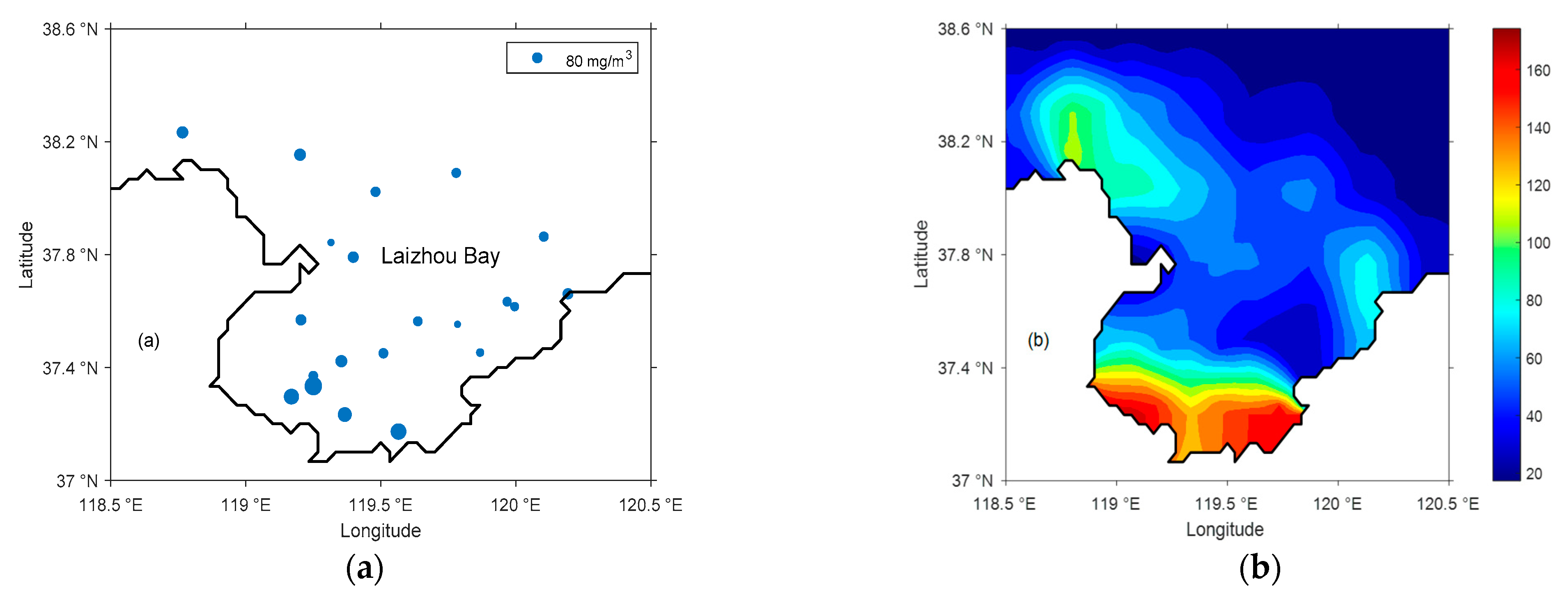
2.4. Model Settings and Observation Data

The calculation area of the model is the Bohai Sea (37–41° N, 117.5–122.5° E). The horizontal resolution is 2’ × 2’ and the ocean is divided into four layers vertically, whose thickness is 5 m, 10 m, 10 m, and 45 m from the top to the bottom, respectively. The simulation time is 15 days with a step of 1 h, which starts at 0:00 on 15th August.
The observed data used in the model came from the simultaneous land–sea survey in Laizhou Bay performed in different seasons from 2018 to 2019, during which petroleum hydrocarbon samples on the sea surface were collected. The pre-treatment and preservation of seawater were carried out in accordance with the Specification for Marine Monitoring (GB 17378.4-2007). The sampling sites of seawater in Laizhou Bay are shown in Figure 1.
The water level data used for validation of the hydrodynamic model were obtained at two stations (Figure 1) from October 2018 to November 2018. The elevation was measured by an RBR-TD at the Longkou station, and the elevation data at Weifang was provided by the long-term monitoring station. The current velocity was measured at five stations (Figure 1). Four of them (C2~C5) were measured using 400 kHz Nortek Aquadopp Profilers (ADCPs) for 26 h with 20-min intervals during a neap tide (12:00 21 October~12:00 22 October) and a spring tide (12:00 30 October~12:00 31 October) in 2018, respectively. During the spring tide, the equipment at station C4 was not working, so the data are missing. The current at station C6 was measured using a current meter in three layers during the same periods with one-hour intervals. The measured current was then vertically averaged for comparison.

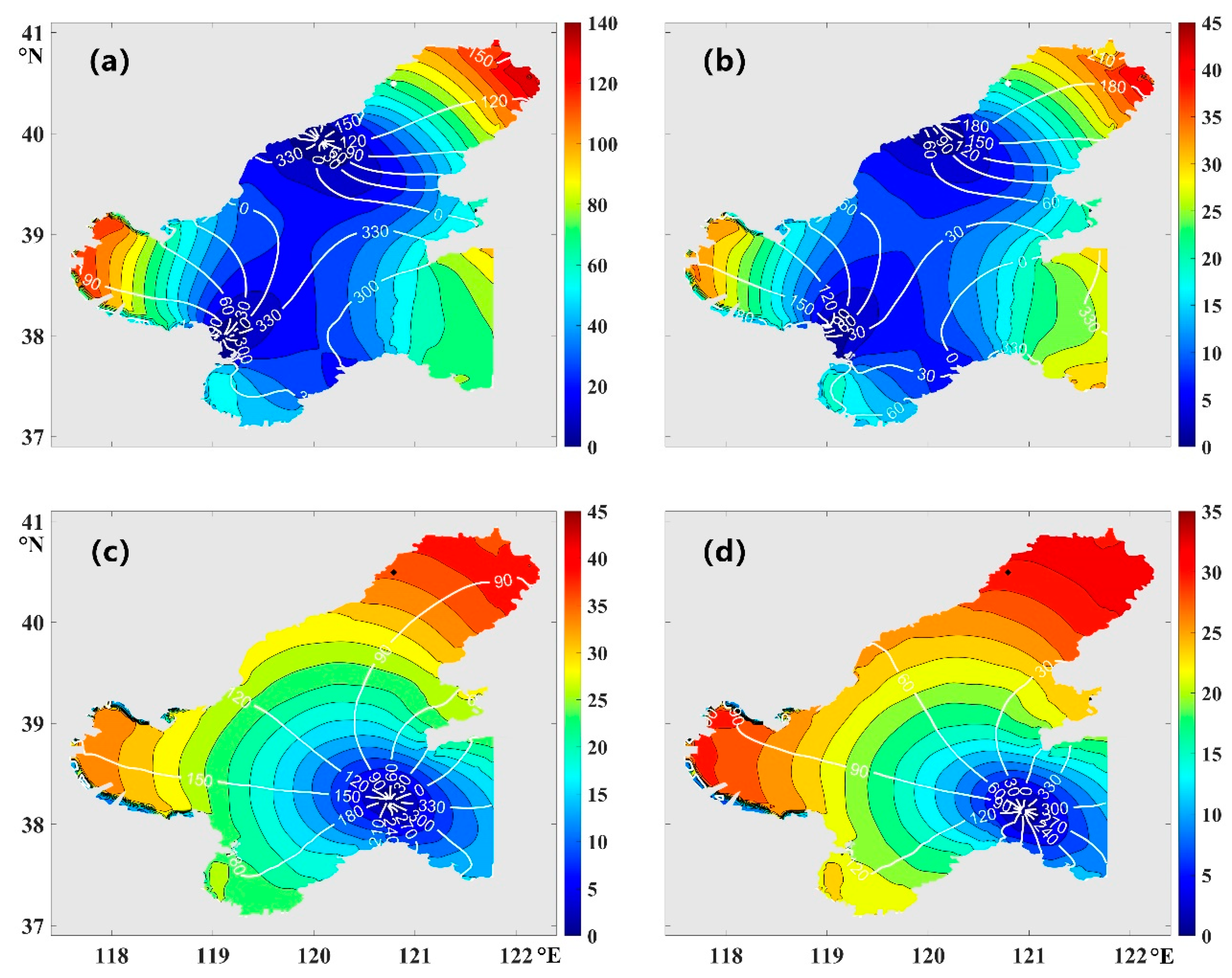
2.5. Hydrodynamic Background Field

In this study, the hydrodynamic background field was provided by the Finite Volume Community Ocean Model (FVCOM), and the calculation area was 37.0–41.0° N, 117.5–122.3° E. The coastline was derived from Landset8 full-band remote sensing data, whose spatial range covered the entire Bohai Sea, and the river runoff was added in the simulated domain. The model adopted an unstructured triangular mesh and 21 sigma layers in the vertical direction. The air–sea interface parameters, such as wind data and other sea surface flux data, came from the reanalyzed ERA5 data in the European Centre for Medium-Range Weather Forecasts (ECMWF), with a horizontal resolution of 0.25° × 0.25° and a temporal resolution of 1 h. Tidal forcing with eight primary partial tides (M2, S2, N2, K2, K1, O1, P1, and Q1) was used at the open boundaries, and was derived from the TPXO8-ATLAS V1 global tidal model provided by the University of Oregon (OSU) in the United States. The initial temperature and salinity field were obtained from the East China Sea model by Ding et al. [21]. The model was cold-started and run for two years for the spin-up, and the hourly output of the third year was used for this study.
The cotidal diagram of the M2, S2, K1, and O1 tides obtained by the model is shown in Figure 2. The harmonic constants of the M2, S2, K1, and O1 tides were compared with the observations using the vector error proposed by Foreman et al. [22]:
D i f f = ( a 0 c o s g 0 a m c o s g m ) 2 + ( a 0 s i n g 0 a m s i n g m ) 2
where ( a 0 ,   g 0 ) and ( a m ,   g m ) denote the observed and simulated amplitude and phase, respectively. The results are shown in Table 1.
The skill score (SS) and correlation coefficient (CC) were used as the quantitative indicators for the model’s validation. The former describes the accuracy of the simulation results, while the latter shows the variation similarity between the simulation and the observation. The SS is calculated as follows:
S S = 1 ( X mod X obs ) 2 ( X obs X obs ¯ ) 2
where Xmod and Xobs denote the modeled and observed variables, respectively, and X ¯ denotes the temporal average of X . The CC is calculated as follows:
C C = ( X mod X mod ¯ ) ( X obs X obs ¯ ) [ ( X mod X mod ¯ ) 2 ( X obs X obs ¯ ) 2 ] 1 2
The results of the above metrics between the observed and simulated water levels and the vertically averaged current velocities are shown in Table 1 and Table 2. A comparison between the observed and simulated current velocities is also shown in Figure 3. These results indicate that the hydrodynamic background field can reproduce the current variation in Laizhou Bay well.
Thus, the hydrodynamic model can provide reliable background currents in Laizhou Bay for inverting the degradation coefficient of petroleum hydrocarbon pollutants.

3. Ideal Twin Experiments

3.1. The Process of Ideal Twin Experiments

The steps of ideal twin experiments can be described as follows:
Step 1. Set an initial estimate value of the parameters in the model.
Step 2. Acquire the ideal ‘observations’ through the forward model.
Step 3. Calculate the cost function that represents the difference between the observation and the simulation.
Step 4. Based on Equation (9), acquire the gradients of the cost function with respect to the parameters of the model and adjust the parameters along the opposite direction of the gradient.
Step 5. When the error meets certain preset conditions, the calculation will stop. Otherwise, go back to step 2 and continue the iteration.
The initial field of petroleum hydrocarbon pollutants with a higher concentration along the coast and a lower concentration offshore was prescribed and is shown in Figure 4a. Regarding the given degradation coefficient of petroleum hydrocarbon pollutants, the superposition of spline functions was applied to preset its initial field. The calculation formula is as follows:
  r i , j = k = 1 N A k ( d i , j , k 2 R 2 l n d i , j , k 2 R + 1 d i , j , k 2 R 2 )
where AK represents the parameter value of the selected point; di,j,k represents the distance between a certain grid point and an independent point; and R represents the influence range of the independent point. The given distribution of the degradation coefficient is shown in Figure 4b, in which the value of the central independent point is 0.100 h−1 and strong degradation occurs in coastal waters.
As for the setting of the degradation coefficient on the time scale, the results of a comprehensive physical–chemical–biological test of the degradation of petroleum hydrocarbon pollutants in Laizhou Bay can be used as a reference and are shown in Figure 5. The decrease in the total petroleum hydrocarbons (TPH) in the control group mainly occurred within 0~20 h, which might have been caused by adsorption and physical volatilization on the wall of the culture vessel. The decrease in the TPH in the systems of “photodegradation + volatilization” (L + V) and “volatile + photodegradation + biodegradation” (V + L + B) occurred mainly within 0~63 h. In conclusion, under different degradation conditions, the TPH shows an exponential trend that decreases rapidly and then basically remains unchanged. Therefore, the degradation coefficient could be viewed as an exponential function descending with time (0~63 h) in subsequent experiments, which could be described as:
r i , j , t = { r i , j , 1 e x p ( 0.143 ( t 1 ) )           1   h t 63   h   0           t > 63   h
where ri,j,k represents the value of the degradation coefficient at time t.

3.2. Results of the Ideal Twin Experiment

According to the numerical experimental tests described above, the uniform independent point scheme with one independent point for every eight grid points at an interval has a better effect, and subsequent experiments were carried out with this scheme. The normalized cost function (NCF) and the mean absolute error (MAE) are vital criteria by which to evaluate the effectiveness of adjoint methods. Here, NCF refers to the cost function obtained in each iteration divided by the one obtained in the first step. The calculation formula for the MAE is presented as:
M A E = i = 1 N | I i P i | N
where N is the number of grids with observations; and I and P denote the model results and given observations, respectively. In this paper, MAE_TPH represents the mean absolute errors between the observation and simulation results for the TPH, while MAE_R represents the mean absolute errors between the given degradation coefficient and simulation results. These evaluation indicators were used to assess the performance of the model in subsequent experiments.

3.2.1. Influence of the Initial Estimate Value on Simulated Results

In the ideal twin experiments, we monitored the convergence of the model by checking the decline in the cost function and terminated the iteration when the change was very slight. Here, we noticed that the convergence speed of the model and the simulation results were closely related to the input of initial estimate value. When the input of initial estimate value is not appropriate, the model requires more iterations to converge, which means a lower calculation efficiency and a larger error in the final inversion results. So, a relevant numerical experiment was designed to determine the optimal value.
Taking the given initial field of the degradation coefficient as a reference, whose value ranges from 0.000 to 0.100 h−1, a series of values in this range were selected as the initial estimates of the model. For comparison, we terminated these experiments after the 30th iteration, and the corresponding MAE results are recorded in Table 3.
When the initial estimate value is set as 0.000 h1, the error in the simulation results reaches the minimum. If the initial estimate value becomes too large, the mean absolute errors keep growing.

3.2.2. Results Analysis

According to the results of the numerical experiments, the initial estimate value of the degradation coefficient was set as 0.00 h−1. Figure 6 shows the trend of evaluation indicators changing with assimilation steps. It can be seen that the NCF tends to be stable after the 20th iteration. Both the MAE_TPH and MAE_R decrease sharply and reach the minimum around the 40th iteration, when the value is significantly decreased relative to the initial value.
In real ocean environments, observations can be contaminated by noises. In this regard, relevant sensitivity experiments were designed in which random perturbations were added to the prescribed observations. The maximum percentages of observation errors are 10%, 20%, and 30% in three experiments, respectively. These noisy “observations” were used instead of the error-free ones, and then we repeated the above ideal twin experiments.
The MAE_TPH and MAE_R of the sensitivity experiments are shown in Table 4. With the growth of the error proportion, the deviation between the inversion results and the ‘observation’ increases correspondingly. Finally, the MAE_R decreases significantly and remains within a narrow range. This shows that the model can resist accidental errors in observations while keeping the results reliable, which indicates its effective utilization of observed data. The results above mean that the inversion results may still be convincing when the adjoint method is adopted in a practical situation.

4. Practical Experiments

The observed data on petroleum hydrocarbons from August, 2019 were used to carry out a practical experiment, which was divided into two main steps:
(a) According to the observed data, the concentration distribution of petroleum hydrocarbons was simulated to obtain the initial field that is as close as possible to the practical observation. The degradation coefficient of petroleum hydrocarbons was not considered in this process.
(b) Taking the result of (a) as the initial field of petroleum hydrocarbon pollutants, the adjoint model was run to invert the degradation coefficient r. After the correction, the initial field of petroleum hydrocarbon pollutants and the distribution of the degradation coefficient r in Laizhou Bay were finally obtained.

4.1. Simulation of the Initial Field of Petroleum Hydrocarbon Pollutants

According to the observations of conventional stations in the Bohai Sea in recent years, the average concentration of petroleum hydrocarbon pollutants is about 24.2 mg /m3. We set this value as the background value of the sea area in the simulation. Similarly, due to the inevitable existence of noise in the practical observations, artificial errors of different proportions were added to the experiment, which account for 5%, 10%, and 20% of the observed values, respectively.
The corresponding MAE_TPH is recorded in Table 5. When the observations do not contain errors, the final value of MAE_TPH decreases to 11.39 mg/m3 after assimilation. Meanwhile, despite the observation errors in different proportions, the MAE_TPH decreases by a considerable percentage after assimilation. Therefore, the initial field of petroleum hydrocarbon pollutants simulated by the adjoint method is reliable and provided a better initial condition for the inversion of the degradation coefficient in the subsequent analysis.

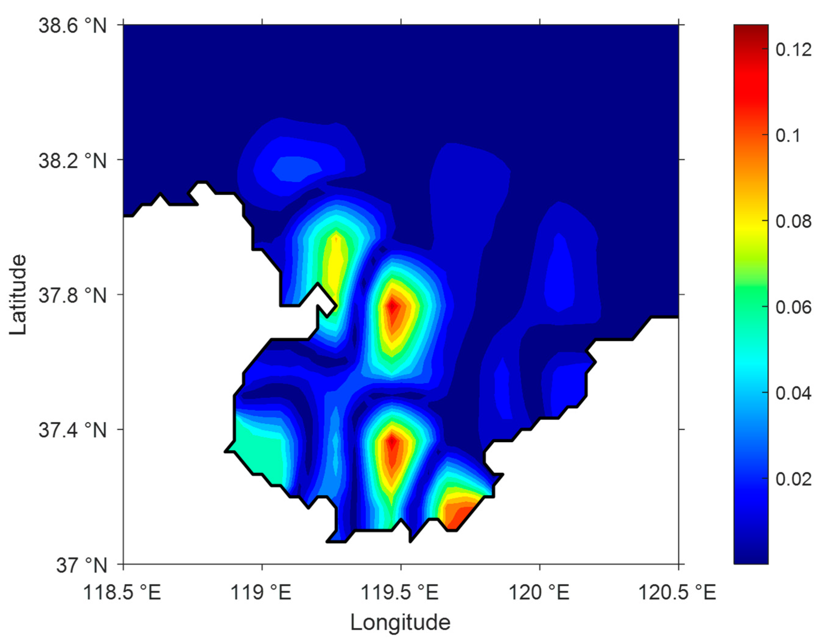
4.2. Analysis of Practical Experimental Results

In step (b), the change in the degradation coefficient on the time scale was set as in Equation (15), which shows an exponential downward trend over a certain period of time. Meanwhile, the initial estimate value of the degradation coefficient r is set as 0.00 h−1. After the adjoint assimilation, the MAE_TPH decreases from 11.39 mg/m3 to 8.61 mg/m3, which shows that the simulation results become closer to the observations, and the inversion of the degradation coefficient r is satisfactory for practical applications.
Figure 8b shows the simulation results after correction of the degradation coefficient, from which the concentration distribution of petroleum hydrocarbon pollutants in Laizhou Bay on 15 August 2019 can be obtained. The concentration of petroleum hydrocarbon pollutants maintains a high level in the surface layer along the southern coast of Laizhou Bay, with the maximum value of 174.0 mg/m3. Meanwhile, it decreases from the southern coast to the interior of the bay. A low-concentration area is formed in the central area of the bay, with the highest concentration not exceeding 60.0 mg/m3. Outside Laizhou Bay, the surface concentration along the northwest and east coasts is higher than those in surrounding waters. Compared with the distribution of observation points in Figure 8a, the simulation results are consistent with the practical observations.
The simulated spatial distribution of the degradation coefficient r at the initial moment is given in Figure 9, which shows a high r value in part of the coastal area and central area of Laizhou Bay, with the maximum value of 0.12 h−1. Compared with Figure 8b, there is no significant positive correlation between the degradation coefficient r and the concentration distribution of petroleum hydrocarbon pollutants. The reason may be that the degraded petroleum hydrocarbons are the majority in some high-concentration areas, while the newly injected petroleum hydrocarbons are the minority. In contrast, the high value of the degradation coefficient r in the nearshore area in Laizhou Bay corresponds to the input of petroleum hydrocarbons from the coastal runoff and the discharge of land-based pollution. Meanwhile, the strong degradation in the central area may be associated with the input of petroleum hydrocarbons caused by marine economic and transportation activities in Laizhou Bay.

5. Conclusions

In this paper, we inverted the spatial distribution of the degradation coefficient of petroleum hydrocarbon pollutants in Laizhou Bay with the adjoint method, in which the transport and degradation model of pollutants was taken as a dynamic constraint. The results of a comprehensive physical–chemical–biological test of the degradation of petroleum hydrocarbon pollutants in Laizhou Bay provided a reference for setting the degradation coefficient on the time scale.
Firstly, the optimal scheme of independent grid points and reasonable initial conditions were determined through numerical experiments. Then, the feasibility and validity of the adjoint method were established with prescribed ‘observations’ in ideal twin experiments. In a practical experiment, the initial field of petroleum hydrocarbon pollutants was simulated, and the error between the simulated results and observations was effectively reduced. Meanwhile, the results were still convincing when noises were added to the observations. On the basis of this initial field, the spatial distribution of the degradation coefficient was inverted, which put the simulation results in better agreement with the observations. Finally, the degradation states of petroleum hydrocarbon pollutants in Laizhou Bay were simulated. The results in the ideal experiment and the practical experiment demonstrate that adjoint assimilation can be an effective method for inverting the degradation coefficient of petroleum hydrocarbon pollutants in Laizhou Bay.

Author Contributions

Conceptualization, X.L. (Xianqing Lv); Methodology, X.L. (Xianqing Lv); Software, S.H. and X.L. (Xiuren Li); Formal analysis, H.H. and D.S.; Investigation, W.S. and S.Z.; Writing—original draft, S.H.; Writing—reviewing and editing, H.H. and D.S.; Supervision, X.L. (Xianqing Lv) and S.Z.; Funding acquisition, S.Z. All authors have read and agreed to the published version of the manuscript.

Funding

This paper was supported by the National key research and development program (2018YFC1407602 and 2019YFC1408405), the National Natural Science Foundation of China (42076011 and U1806214), the Shandong Provincial Natural Science Foundation, China (ZR2019MD010), and the Innovation and Strengthen Project of Guangdong Province (Grant No. 2018KQNCX082).

Conflicts of Interest

The authors declare no conflict of interest.

References

  1. Xing, Q.; Meng, R.; Lou, M.; Bing, L.; Liu, X. Remote Sensing of Ships and Offshore Oil Platforms and Mapping the Marine Oil Spill Risk Source in the Bohai Sea. Aquat. Procedia 2015, 3, 127–132. [Google Scholar] [CrossRef]
  2. Walsh, J.; Lenes, J.; Darrow, B.; Parks, A.; Weisberg, R.; Zheng, L.; Hu, C.; Barnes, B.; Daly, K.; Shin, S.-I.; et al. A simulation analysis of the plankton fate of the Deepwater Horizon oil spills. Cont. Shelf Res. 2015, 107, 50–68. [Google Scholar] [CrossRef]
  3. Makri, P.; Stathopoulou, E.; Hermides, D.; Kontakiotis, G.; Zarkogiannis, S.D.; Skilodimou, H.D.; Bathrellos, G.D.; Antonarakou, A.; Scoullos, M. The Environmental Impact of a Complex Hydrogeological System on Hydrocarbon-Pollutants’ Natural Attenuation: The Case of the Coastal Aquifers in Eleusis, West Attica, Greece. J. Mar. Sci. Eng. 2020, 8, 1018. [Google Scholar] [CrossRef]
  4. Paul, J.H.; Hollander, D.; Coble, P.; Daly, K.L.; Murasko, S.; English, D.; Basso, J.; Delaney, J.; McDaniel, L.; Kovach, C.W. Toxicity and Mutagenicity of Gulf of Mexico Waters During and After the Deepwater Horizon Oil Spill. Environ. Sci. Technol. 2013, 47, 9651–9659. [Google Scholar] [CrossRef] [PubMed]
  5. Xu, M.; Chua, V.P. A numerical study on land-based pollutant transport in Singapore coastal waters with a coupled hydrologic-hydrodynamic model. J. Hydro-Environ. Res. 2017, 14, 119–142. [Google Scholar] [CrossRef]
  6. Snyder, K.; Mladenov, N.; Richardot, W.; Dodder, N.; Nour, A.; Campbell, C.; Hoh, E. Persistence and photochemical transformation of water soluble constituents from industrial crude oil and natural seep oil in seawater. Mar. Pollut. Bull. 2021, 165, 112049. [Google Scholar] [CrossRef]
  7. Chen, C.S.; Liu, H.D.; Beardsley, R.C. An unstructured grid, finite-volume, three-dimensional, primitive equations ocean model: Application to coastal ocean and estuaries. J. Atmos. Ocean. Technol. 2003, 20, 159–186. [Google Scholar] [CrossRef]
  8. Wang, S.-D.; Shen, Y.-M.; Guo, Y.-K.; Tang, J. Three-dimensional numerical simulation for transport of oil spills in seas. Ocean Eng. 2008, 35, 503–510. [Google Scholar] [CrossRef]
  9. Zhao, X.; Wang, X.; Shi, X.; Li, K.; Ding, D. Environmental capacity of chemical oxygen demand in the Bohai Sea: Modeling and calculation. Chin. J. Oceanol. Limnol. 2011, 29, 46–52. [Google Scholar] [CrossRef]
  10. Zhao, L.; Wei, H.; Xu, Y.; Feng, S. An adjoint data assimilation approach for estimating parameters in a three-dimensional ecosystem model. Ecol. Model. 2005, 186, 235–250. [Google Scholar] [CrossRef]
  11. Li, X.Y.; Wang, C.H.; Lv, X.Q. Estimation of the Parameters in a Dynamical Marine Ecosystem Model Based on the Adjoint Assimilation. Appl. Mech. Mater. 2013, 321–324, 2419–2423. [Google Scholar] [CrossRef]
  12. Wang, C.; Li, X.; Lv, X. Numerical Study on Initial Field of Pollution in the Bohai Sea with an Adjoint Method. Math. Probl. Eng. 2013, 2013, 104591. [Google Scholar] [CrossRef] [Green Version]
  13. Han, B.; Liu, A.; Wang, S.; Lin, F.; Zheng, L. Concentration level, distribution model, source analysis, and ecological risk assessment of polycyclic aromatic hydrocarbons in sediments from laizhou bay, China. Mar. Pollut. Bull. 2020, 150, 110690. [Google Scholar] [CrossRef] [PubMed]
  14. Zhang, M.; Yu, G.; Wang, F.; Li, B.; Han, H.; Qi, Z.; Wang, T.; Qi, Z. Terrestrial dissolved organic carbon consumption by heterotrophic bacterioplankton in the Huanghe River estuary during water and sediment regulation. J. Oceanol. Limnol. 2018, 37, 1062–1070. [Google Scholar] [CrossRef]
  15. Hu, N.J.; Shi, X.F.; Huang, P.; Liu, J.H. Polycyclic aromatic hydrocarbons in surface sediments of Laizhou Bay, Bohai Sea, China. Environ. Earth Sci. 2010, 63, 121–133. [Google Scholar] [CrossRef]
  16. Zheng, Q.; Li, X.; Lv, X. Application of Dynamically Constrained Interpolation Methodology to the Surface Nitrogen Concentration in the Bohai Sea. Int. J. Environ. Res. Public Health 2019, 16, 2400. [Google Scholar] [CrossRef] [Green Version]
  17. Zong, X.; Xu, M.; Xu, J.; Lv, X. Improvement of the ocean pollutant transport model by using the surface spline interpolation. Tellus A Dyn. Meteorol. Oceanogr. 2018, 70, 1–13. [Google Scholar] [CrossRef] [Green Version]
  18. Lv, X.; Zhang, J. Numerical study on spatially varying bottom friction coefficient of a 2D tidal model with adjoint method. Cont. Shelf Res. 2006, 26, 1905–1923. [Google Scholar]
  19. Pan, H.; Guo, Z.; Lv, X. Inversion of Tidal Open Boundary Conditions of the M2 Constituent in the Bohai and Yellow Seas. J. Atmos. Ocean. Technol. 2017, 34, 1661–1672. [Google Scholar] [CrossRef]
  20. Fan, W.; Lv, X. Data assimilation in a simple marine ecosystem model based on spatial biological parameterizations. Ecol. Model. 2009, 220, 1997–2008. [Google Scholar] [CrossRef]
  21. Ding, Y.; Bao, X.; Yao, Z.; Song, D.; Song, J.; Gao, J.; Li, J. Effect of coastal-trapped waves on the synoptic variations of the Yellow Sea Warm Current during winter. Cont. Shelf Res. 2018, 167, 14–31. [Google Scholar] [CrossRef]
  22. Foreman, M.G.G.; Henry, R.F.; Walters, R.A.; Ballantyne, V.A. A finite element model for tides and resonance along the north coast of British Columbia. J. Geophys. Res. Space Phys. 1993, 98, 2509–2531. [Google Scholar] [CrossRef]
Figure 1. Seawater sampling sites in Laizhou Bay.
Jmse 09 00655 g001
Figure 2. The cotidal chart of each constituent. (a) M2, (b) S2, (c) K1, and (d) O1.
Jmse 09 00655 g002
Figure 3. Comparison between the observed (red dots) and modeled (black line) current velocities at the (a) C2, (c) C3, (e) C5, and (g) C6 stations during the neap tide and at the (b) C2, (d) C3, (f) C5, and (h) C6 stations during the spring tide.
Jmse 09 00655 g003
Figure 4. (a) The given distribution of petroleum hydrocarbon pollutants (unit: mg/m3). (b) The given distribution of the degradation coefficient (unit: h−1).
Jmse 09 00655 g004
Figure 5. Variation of TPH with time under different conditions in Laizhou Bay. “Control” denotes the control group. “V + L” denotes the condition of “photodegradation + volatilization”. “V + L + B” denotes the condition of “volatilization + photodegradation + biodegradation”.
Jmse 09 00655 g005
Figure 6. (a) Decline of NCF with assimilation steps; (b) Decline of MAE_TPH with assimilation steps; (c) Decline of MAE_R with assimilation steps. Based on Table 4, MAE_TPH, which represents the deviation between the inversion results and the “observation”, decreases from 18.37 mg/m3 to 0.13 mg/m3. The MAE_R decreases from 2.56 × 10⁻² h−1 to 2.97 × 10⁻³ h−1 with the decline percentage of 88.40%. Figure 7a,b respectively show the given distribution and inversion result of the degradation coefficient. In terms of the overall distribution, the inversion result is close to the given initial field, in which the degradation degree of petroleum hydrocarbons in Laizhou Bay is higher than that far away from the coast. Figure 7c shows the absolute value of the difference between the inversion results and the given distribution. Except for the southwest part of the sea area, the deviation degree between them in Laizhou Bay remains at a low level, meaning that the final inversion results are almost identical to the given distribution.
Jmse 09 00655 g006
Figure 7. (a) Map of the given distribution of the degradation coefficient. (unit: h−1); (b) Map of the inversion result in ideal twin experiments (unit: h−1); (c) Map of the absolute value of the difference between the inversion result and the given distribution (unit: h−1).
Jmse 09 00655 g007
Figure 8. (a) Observation points in Laizhou Bay in August 2019 (the dot size indicates the concentration of petroleum hydrocarbons); (b) The simulated concentration distribution of petroleum hydrocarbons in Laizhou Bay on 15 August 2019 (unit: mg/m3).
Jmse 09 00655 g008
Figure 9. Map of the simulated spatial distribution of the degradation coefficient r at the initial moment (unit: h−1).
Jmse 09 00655 g009
Table 1. Model validation for water levels.
Tide StationsDiffSSCC
M2S2K1O1
Longkou0.035 0.018 0.024 0.018 0.920.96
Weifang0.049 0.027 0.011 0.022 0.940.97
Table 2. Model validation for current velocities.
StationSSCC
UVUV
C2 neap0.290.910.730.92
C3 neap0.820.900.910.95
C4 neap0.880.670.920.89
C5 neap0.870.790.910.91
C6 neap0.630.900.870.94
C2 spring0.620.960.820.95
C3 spring0.850.930.940.93
C5 spring0.860.700.910.91
C6 spring0.800.580.900.91
Table 3. Mean absolute errors in the TPH (MAE_TPH) and degradation coefficient (MAE_R) corresponding to different initial estimate values.
Initial Guess ValueMAE_TPH (mg/m3)MAE_R (h−1)
0.000.162.97 × 10−3
0.03 × 10−10.193.15 × 10−3
0.05 × 10−10.253.25 × 10−3
0.010.363.86 × 10−3
0.020.665.89 × 10−3
0.051.661.33 × 10−2
0.083.352.46 × 10−2
0.104.213.19 × 10−2
Table 4. The decrease in MAE_TPH and MAE_R corresponding to different observation errors in sensitivity experiments.
Percent ErrorsInitial Value of MAE_TPH (mg/m3)Final Value of MAE_TPH (mg/m3)Initial Value of MAE_R (h−1)Final Value of MAE_R (h−1)Decline Percent of MAE_R
0%18.370.132.56 × 10−22.97 × 10−388.40%
5%18.371.352.56 × 10−24.19 × 10−383.63%
10%18.372.212.56 × 10−25.83 × 10−377.23%
20%18.373.412.56 × 10−28.10 × 10−368.36%
Table 5. MAE_TPH in the practical experiment.
Percent ErrorsInitial Value of MAE_TPH (mg/m3)Final Value of MAE_TPH (mg/m3)Decline Percent of MAE_TPH
0%52.6911.3978.38%
5%52.6911.9977.24%
10%52.6913.9173.60%
20%52.6919.4663.07%
Publisher’s Note: MDPI stays neutral with regard to jurisdictional claims in published maps and institutional affiliations.

