Article

Modified Vector Field Path-Following Control System for an Underactuated Autonomous Surface Ship Model in the Presence of Static Obstacles

Centre for Marine Technology and Ocean Engineering (CENTEC), Instituto Superior Técnico, Universidade de Lisboa, Av. Rovisco Pais, 1049-001 Lisboa, Portugal
*
Author to whom correspondence should be addressed.
J. Mar. Sci. Eng. 2021, 9(6), 652; https://doi.org/10.3390/jmse9060652
Submission received: 5 May 2021 / Revised: 28 May 2021 / Accepted: 3 June 2021 / Published: 12 June 2021
(This article belongs to the Special Issue Maritime Autonomous Vessels)

Abstract

:
A modified path-following control system using the vector field method for an underactuated autonomous surface ship model is proposed in the presence of static obstacles. With this integrated system, autonomous ships are capable of following the predefined path, while avoiding the obstacles automatically. It is different from the methods in most published papers, which usually study path-following and obstacle collision avoidance, separately. This paper considers the coupled path following and collision avoidance task as a whole. Meanwhile, the paper also shows the heading control design method in the presence of static obstacles. To obtain a strong stability property, a nonlinear autopilot is designed based on the manoeuvring tests of the free-running ship model. The equilibrium point of the controller is globally exponentially stable. For the guidance system, a novel vector field method was proposed, and the proof shows the coupled guidance and control system is uniform semi-global exponentially stable (USGES). To prevent the obstacles near the predefined path, the proposed guidance law is augmented by integrating the repelling field of obstacles so that it can control the ship travel toward the predefined path through the obstacles safely. The repelling field function is given considering the obstacle shape and collision risk using the velocity obstacle (VO) algorithm. The simulations and ship model test were performed to validate the integrated system of autonomous ships.

1. Introduction

Autonomous ships have been drawing significant attention recently. The most important reasons for the rapid development of autonomous ships are safety and economic benefit. The risk of maritime transportation is quantified based on various types of total ship losses [1], but as reported by Allianz Global Corporate and Specialty [2], about 75% to 96% of marine accidents can be ultimately attributed to human error. Autonomous shipping can significantly improve safety by reducing human factors.
For autonomous vehicles, the guidance system and control system are two basic low-level systems. They are closely related to transient motion behaviour, such as path following [3], path tracking [4], and path manoeuvring [5]. Therefore, there are two fundamental systems that determine the overall performance [6]. The fundamental requirement of autonomous ships is that they can follow the predefined path fully autonomously or remotely. Guidance systems calculate the desired course or heading angles for the autonomous ships. Their objective is to guide the ships approaching the desired path.
One of the most widely used guidance laws for autonomous ships is line of sight (LOS). It has been reported in many papers, as can be seen in [7,8,9,10,11,12,13]. The classical LOS is a typical three-points geometry method [6]. A constant look-ahead distance usually needs to be previously defined for LOS. To improve the robustness, it can also be defined as a function of the cross-track error [14]. Follow-up work can be found in [15]. The LOS was also used for the positioning control of the over-actuated autonomous underwater vehicle (AUV) under the effects of ocean current and model uncertainties in [16,17]. A revised version, integral LOS, was proposed to compensate for the environmental disturbance in [16,17,18,19], and its stability was also proved. Considering the varying environmental disturbance, Fossen and Lekkas [20] proposed an adaptive ILOS for the path-following control of marine ships.
The vector field guidance law is a mathematical method. The main idea is to build a vector space, where all the vectors point to the path smoothly. Therefore, if the ship follows the vectors in the space, it will converge to the predefined path finally. Compared with the LOS guidance law, the vector field is a mathematical method with a flexible structure. For the vector field methods, only a vector function needs to be defined, meanwhile, it can also be designed with the specific tasks, for example, collision or desired direction. It was widely used for unmanned aerial vehicles [21,22,23,24]. For example, Lawrence et al. [25] proposed a Lyapunov-based vector field and proved the global asymptotic stability. Global uniform bounded stability of vector field guidance law of an unmanned aerial vehicle (UAV) following arbitrary curves was proved by Wang et al. [26]. Recently, it was modified and employed for the path-following control of marine ships and underwater vehicles [27,28,29].
For a closed-loop control system, the global exponential stable (GES) is the strongest property [30,31], because it can guarantee additional robustness and performance properties of the control system. However, it cannot be achieved for marine ships, because the error dynamic function is local [32,33,34]. Fossen and Pettersen [32] presented a uniform semi-global exponential stability (USGES) proof for the line-of-sight (LOS) guidance law, and the proof extended the previous results that only guarantee global–exponential stability [34]. In this paper, a time-varying vector field guidance law is proposed, and the equilibrium point is uniform semi-global exponential stable.
For marine surface ships, it is inevitable to encounter obstacles at sea. A collision avoidance system is one of the basic systems for autonomous ships because it makes the ship capable of taking action to local sensor information, [35,36]. It also guarantees that the ship sails safely in unknown or dynamic environments. To improve the safety of autonomous ships, an intelligent decision-making system using fuzzy logic was proposed by Perera et al. [37,38,39]. Statheros et al. [40] summarized the recent works on collision avoidance for autonomous vehicles. The velocity obstacle (VO) algorithm was employed to prevent the collision of marine ships at seas by Huang et al., [41,42]. Kuwata et al. [43] extended the VO for the ship’s navigation by considering the International Regulations for Preventing Collisions (COLREGs). Mou et al. [44] proposed a collision-avoidance system based on the collected AIS data.
The contribution of this paper is to extend the vector field path-following control system for an underactuated autonomous surface ship model in the presence of static obstacles. The proposed system considers the coupled path-following and collision avoidance task as a whole. It is different from the most well-established methods in the literature, where the path-following control and collision avoidance control are usually treated separately. Classical collision avoidance usually emphasized on the minimize the collision risk by assuming the ship are fully controlled. However, few papers explore the autopilot design for autonomous ships in the presence of static obstacles. In this paper, a nonlinear heading controller was designed considering the manoeuvrability of the underactuated surface ship. While different forms of sliding mode controllers have been used [26], a classical sliding mode controller with global exponential stability (GES) is employed here. For the guidance system, a time-varying vector field guidance law was proposed and proved to be uniform semi-global exponential stable (USGES). This guidance law was extended using a risk-based repelling field method. The resulted guidance laws can control the ship to avoid obstacles near the path. The proposed system generates the repelling vectors around the obstacle, which guide the ship to travel away from the obstacles. The repelling field function is given considering the obstacle shape and collision risk using the velocity obstacle (VO) algorithm.

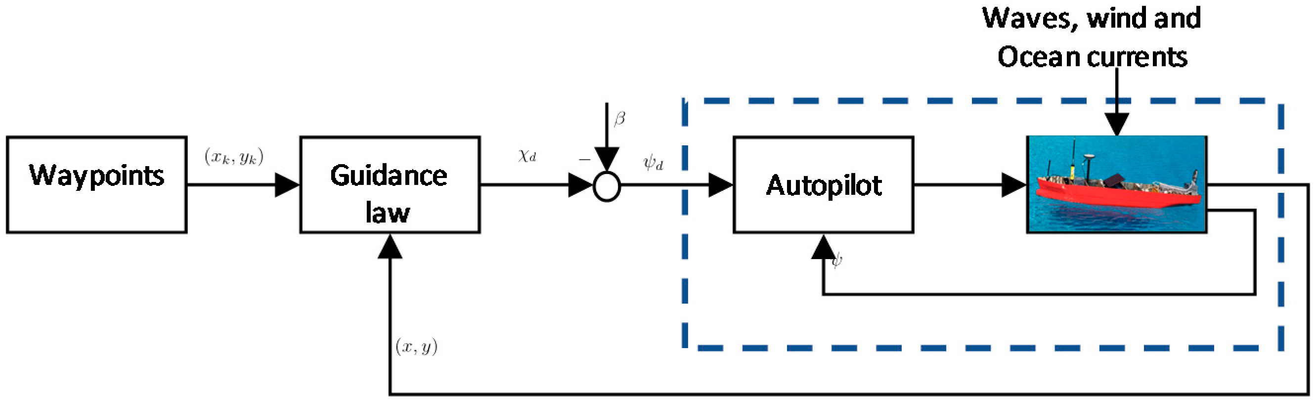
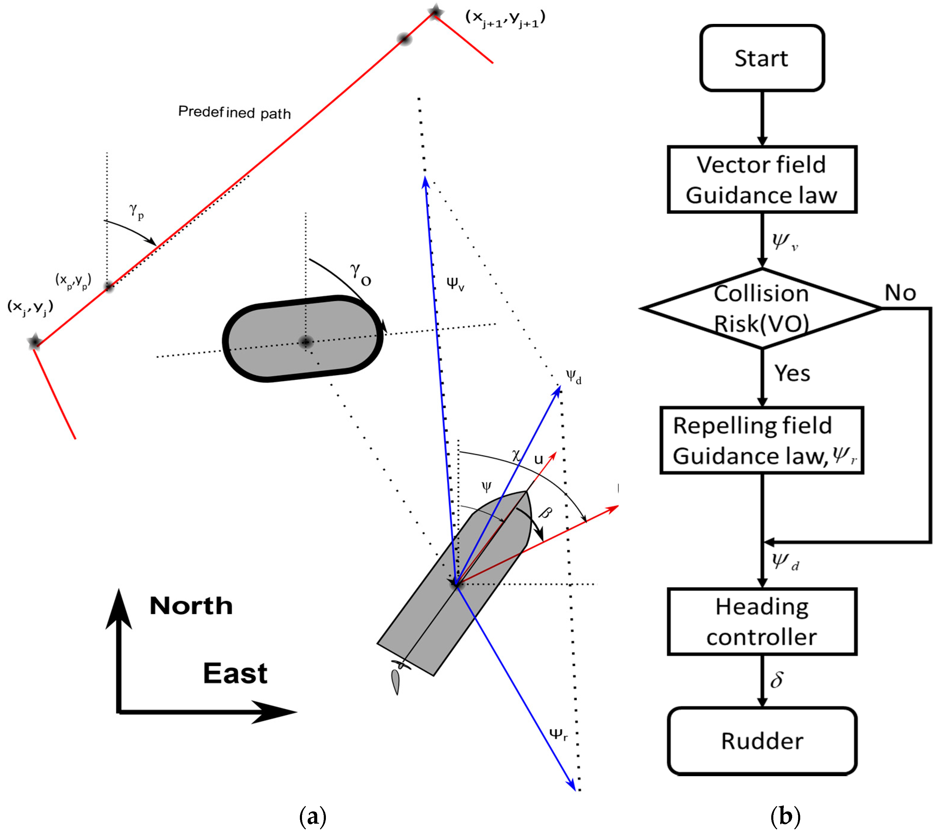
2. Path-Following Control System

This section will briefly describe the kinematics and control objects of the path-following of marine ships. As presented in Figure 1, a typical control system includes the guidance law and autopilot. The guidance law provides the desired angle for the autopilot, and the autopilot will steer the rudder of the ship to track the path.
Without a loss of generality, a straight path-following control system for marine autonomous surface ships is considered, as presented in Figure 2. In order to simplify the problem, some assumptions and physical constraints were made:
Assumption 1.
The motion of the ship is described in three degrees of freedom: surge, sway and yaw.
Assumption 2.
The ship is underactuated in its configuration space.
Assumption 3.
The ship is treated as a rigid body and the maximum rudder angle is 35 degrees.
From Figure 2, the cross-track error can be calculated:
[ 0 y e ] = R T ( γ p ) [ x ( t ) x p ( t ) y ( t ) y p ( t ) ]
where ( x ( t ) , y ( t ) ) is the ship’s position at time t. ( x p ( t ) , y p ( t ) ) is the orthogonal projection of the ship’s position on the predefined path. The R ( γ p ) is the rotation matrix [45], given:
R ( γ p ) = [ cos ( γ p ) sin ( γ p ) sin ( γ p ) cos ( γ p ) ] S O
The cross-track error ye can be obtained from Equation (1):
y e ( t ) = ( x ( t ) x p ( t ) ) sin ( γ p ) + ( y ( t ) y p ( t ) ) cos ( γ p )
Obviously, the control object is to make the cross-track error converge towards zero. It is given as follows:
lim t + y e ( t ) = 0
The kinematic equation of the motion of ships is given as
x ˙ = u cos ( ψ ) v sin ( ψ ) y ˙ = u sin ( ψ ) + v cos ( ψ ) ψ ˙ = r
where ψ is the yaw angle. Differentiation of (3), and further simplified by substituting (5), results as
y ˙ e = U sin ( ψ γ p + β )
where the phase β is the drift angle [6]. U is the ground speed of a ship, ( U = u 2 + v 2 ). For notational simplicity, the time t is omitted.
To obtain strong stability properties, a nonlinear sliding mode controller based on the first-order nonlinear Nomoto model was used for the heading control. The Nomoto model with bounded bias term is given [46]:
T r ˙ + n 3 r 3 + n 1 r = K δ + b 0
where b0bmax is a bounded bias term. K , T , n 3   and   n 1 are the Nomoto constants. δ is the rudder angle. Notice that, n 1 = 1 for a stable ship. The parameters can be obtained using the free-running model test in real-time [47]. With the Nomoto model, the sliding surface is defined as
s : = ( d d t + λ ) 2 ( 0 t ψ ˜ ( τ ) d τ ) = ψ ˜ ˙ + 2 λ ψ ˜ + λ 2 0 t ψ ˜ ( τ ) d τ : = s ˙ 0 + λ s 0
where s 0 = ψ ˜ + λ 0 t ψ ˜ ( τ ) d τ . ψ ˜ is the heading error. λ is a constant [6]. Assume that σ:= r−s, and substitute it into (7) gives:
T s ˙ = K δ T σ ˙ ( n 3 r 2 + n 1 ) ( σ + s ) + b 0
Then, the control law can be obtained as
δ = 1 K ( T σ ˙ + ( n 3 r 2 + n 1 ) σ K d s η sgn ( s ) )
where Kd > 0 is the feedback control gain. ηbmax is a positive design gain [30]. The Lyapunov function can be used to prove that the equilibrium point is globally exponentially stable (GES) (Theorem 4.10 in [29]). The detailed proof can be found in [6,22,48].
In this part, Nomoto parameters will be estimated using system identification based on the manoeuvring tests. The free-running manoeuvring tests were carried out using a scaled ship model (1/65.7) with one propeller and one rudder, as presented in Figure 3. The ship is 2.58 m in length, and 0.43 m in breadth. The designed draft is 0.14 m.
To measure the motion of the ship, various sensors and actuators were used and synchronized using the LabView platform. LabView is a graphical programming environment widely used for data acquisition and control application. It includes the software platform and hardware.
Here, a compactRIO with various modules are used in the free-running ship model. The typical sensors, such as an internal measurement unit, yaw rate sensor, electrical motors, server motor industrial Wi-Fi unit, are given in Figure 4.
The 20 20 zigzag manoeuvring tests, as suggested by ITTC [49], were conducted in the tank of Laboratory National de Civil Engineering (LNEC). The results are presented in Figure 5. Then, the least square support vector machine (LS-SVM), [50,51], was employed to identify the parameters. More details can be found in [46]. One test is used to estimate the parameters, as shown in Figure 5a. The results agree well with the training test. The obtained values of the Nomoto parameters are given: T = 7.7515, n3 = 0.0669, K = 0.1129. To validate the results, a new 20 20 zigzag manoeuvring test was chosen as a test set. This test was not used for the training. The validation result is presented in Figure 5b. The prediction agrees well with the tests. In the training and validation process, the heading angle is the integration of the yaw rate, which is the prediction of the obtained Nomoto model. Therefore, in order to eliminate the accumulated error due to the integration, one step prediction is adopted when calculating the yaw heading.

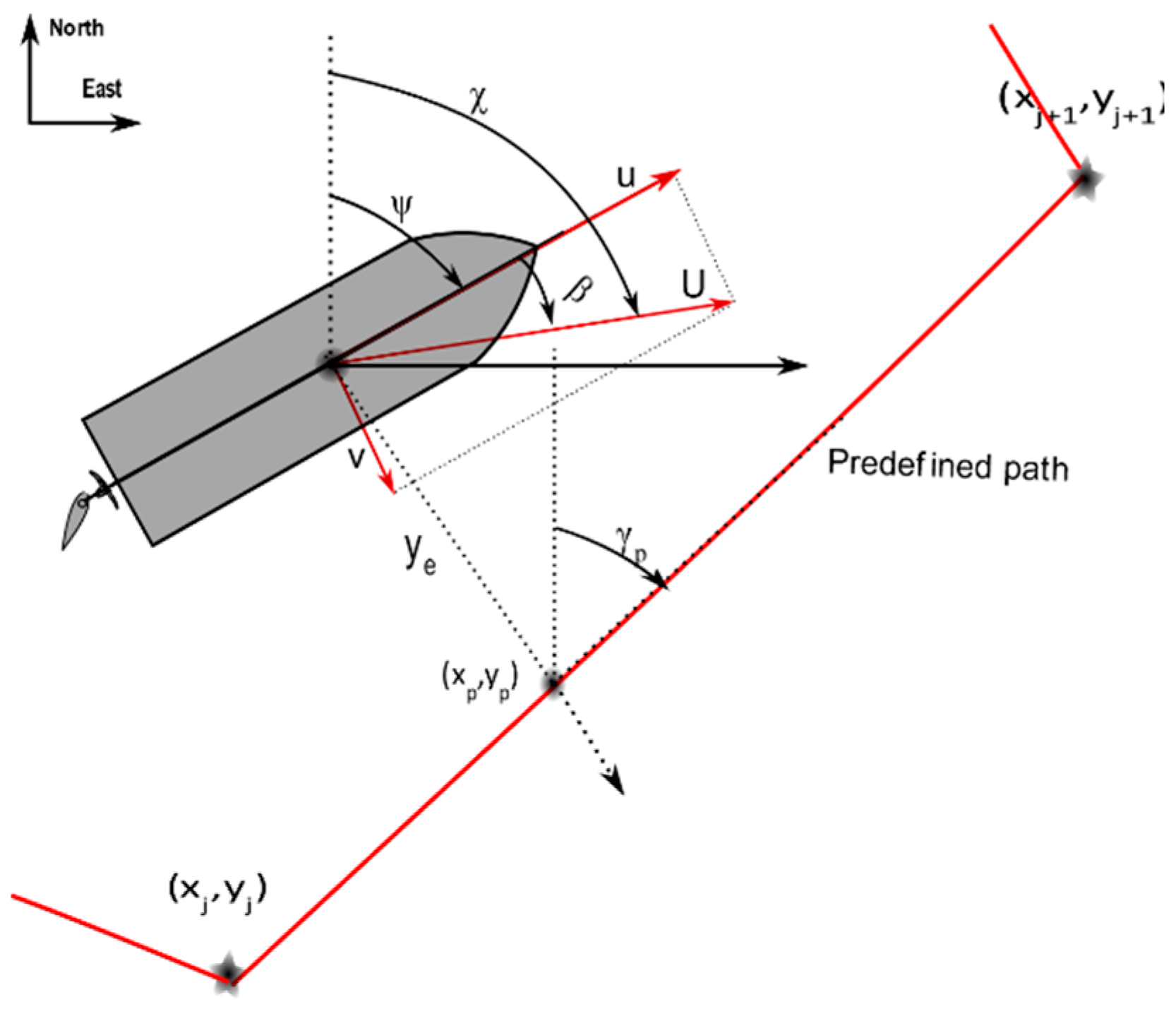
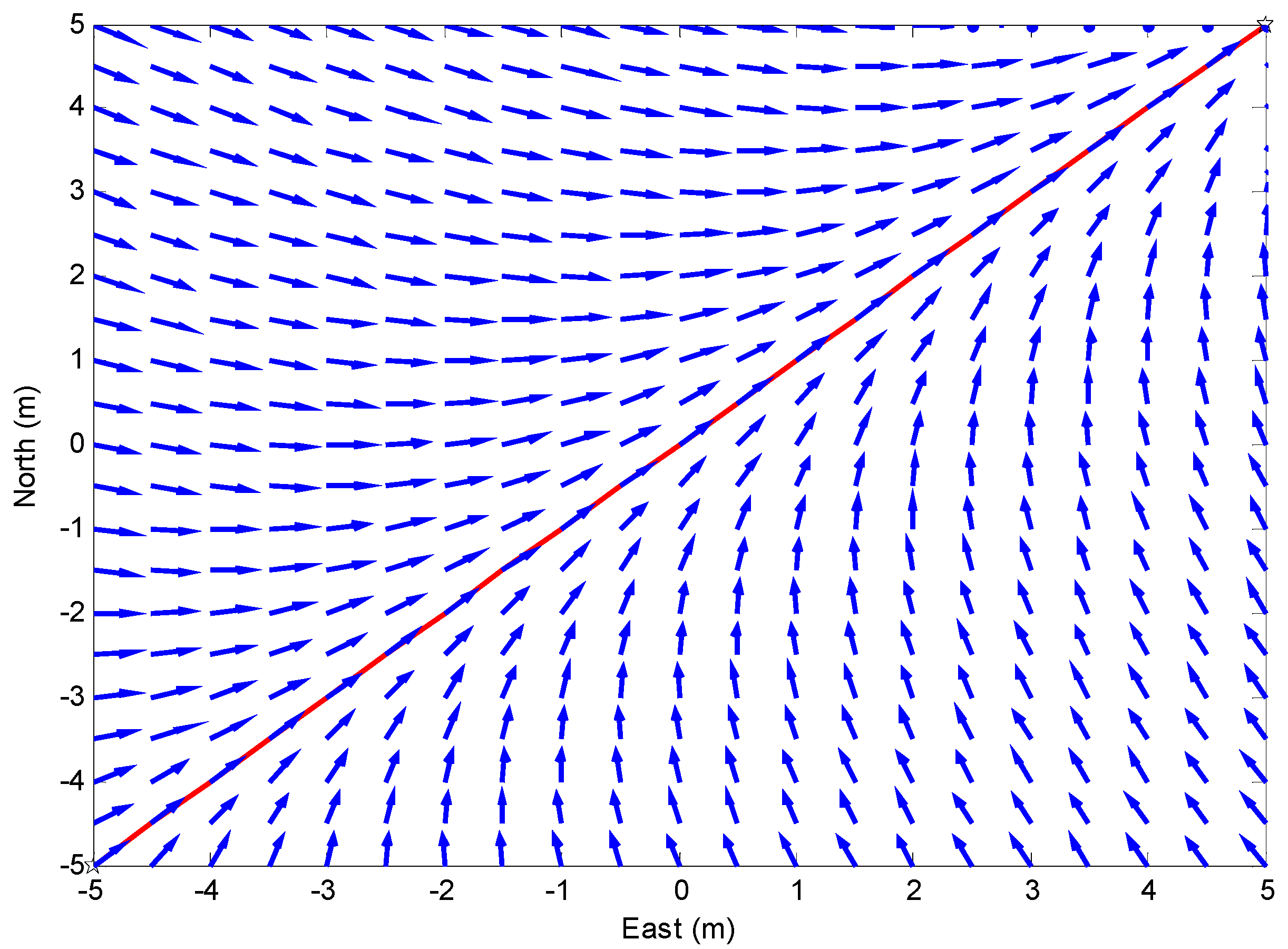
3. Time-Varying Vector Field Guidance Law

As discussed above, the guidance system plays an important role in autonomous ships. It calculates the desired heading or course angle based on the orthogonal distance between the ship and the path. In a simple word, the guidance law plays the same role as an experienced sailor. In this section, a vector field guidance law is used for the path-following control of the underactuated marine surface ship. The vector field method is a novel guidance law for marine ships. Its main principle is to generate vector space around the path to be followed, and all the vectors point to the path smoothly, as presented in Figure 6. The vectors usually denote the desired travelling direction (course angle) for the autonomous vessels. If the ship follows the vectors, it will ultimately converge to the predefined path.
The function for the generation of vectors is important because it determines the quality of the vectors, such as the distribution and strength of vectors, the convergence rate, etc. Meanwhile, it also indirectly determines the performance of the guidance system of underactuated autonomous ships. Here, a vector field is given:
ψ d = γ p sgn ( y e ) tan 1 ( ( | y e | Δ ) θ ( t , y e ) ) β
where θ ( t , y e ) is a time-varying function, ∆ > 0 is a constant, and Δ min Δ Δ max .
As discussed above, the low-level controller is GES and can track the desired heading angle perfectly. Then, substituting (11) into (6) gives:
y ˙ e = sgn ( y e ) U sin ( tan 1 ( ( | y e | Δ ) θ ( t , y e ) ) )
It can be further simplified as
y ˙ e = sgn ( y e ) U | y e | θ ( t , y e ) Δ 2 θ ( t , y e ) + | y e | 2 θ ( t , y e )
To prove the stability of the guidance law, the Lyapunov method is used and the Lyapunov candidate is:
V 1 ( t , y e ) = 1 2 y e 2
The time derivative is:
V ˙ 1 ( t , y e ) = sgn ( y e ) y e U | y e | θ ( t , y e ) Δ 2 θ ( t , y e ) + | y e | 2 θ ( t , y e ) = U | y e | θ ( t , y e ) + 1 Δ 2 θ ( t , y e ) + | y e | 2 θ ( t , y e ) 0
Since V 1 ( t , y e ) > 0 and V ˙ 1 ( t , y e ) 0 , according to Theorem 4.8 by Khalil [30], the equilibrium point is uniformly stable. As discussed in [48,52], the function, θ ( t , y e ) , must guarantee that the function Φ ( t , y e ) = | y e | θ ( t , y e ) 1 is positive and lower-bounded, then the equilibrium point ye = 0 is uniform semi-global exponential stable (USGES) (Definition 2.7 by Loría and Panteley [31]). In this paper, the function is defined as θ ( t , y e ) = 0.4 | y e | + 1 and the function Φ ( t , y e ) = | y e | 0.4 | y e | e 2 5 e 0.86 > 0 is positive and lower-bounded. The cross-track error, y e , depends on the initial error and then decreases exponentially with time.

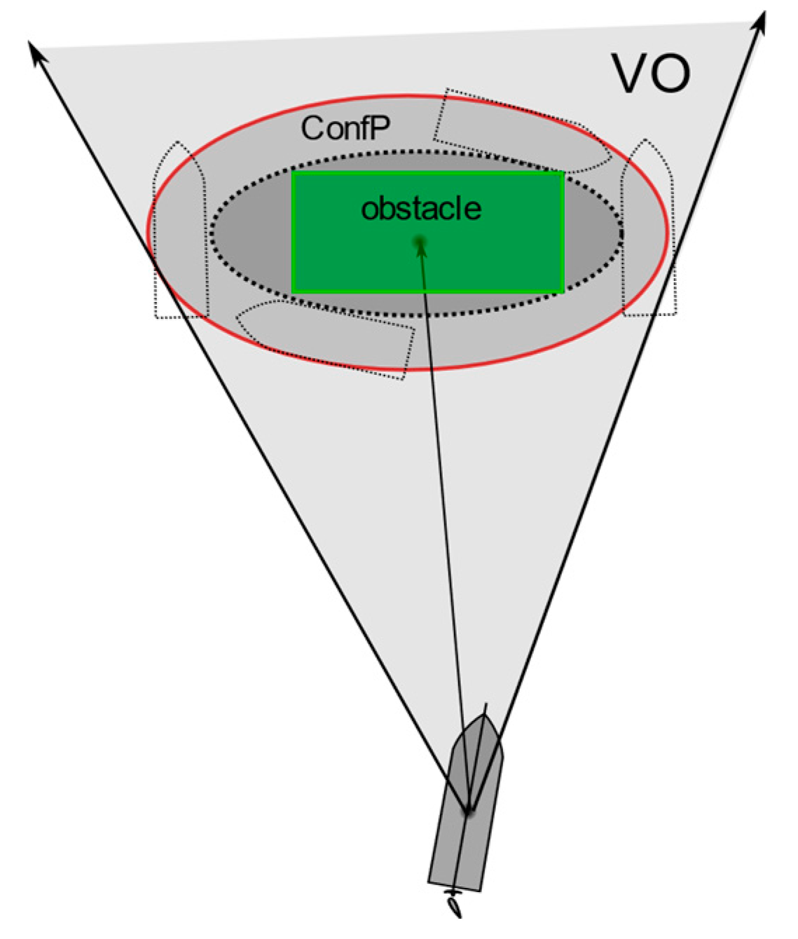
4. Risk-Based Obstacle Collision Avoidance System

An obstacle avoidance control system is proposed for autonomous surface ships. Usually, the desired path should be planned with a global world map, so the ship can travel safely. However, it cannot neglect the obstacle near the path, which was not displayed on the map, for example, large sea animals or floating marine structure, etc. The obstacle avoidance system can make the autonomous ship respond to the dynamic local sensor information and guide the ship safely to avoid the obstacles.
Assuming that there is one obstacle near the path, to avoid the obstacle, the directions of the vector need to be changed. Here, a repelling field function is used to generate the vector with the angle, ψ r . When the ship is near the obstacle, the vector will control the ship travel away from the obstacle with the aid of the heading controller.
Figure 7 shows the principle of the collision avoidance system for autonomous surface ships. A repelling field function is used to generate a heading angle ψ r . If neglecting the path-following task, the ship tracks this heading angle ψ r , which will guide the ship to travel away from the obstacle. Meanwhile, the vector field guidance law will generate the heading angle ψ v which attracts the ship moving toward the path. The final resulted heading angle, ψ d = ψ r + ψ v , is given in Figure 7. Obviously, the repelling function needs to be defined carefully, so the ship can travel toward the path smoothly, and meanwhile, avoiding the obstacle. The repelling function is given as
ψ r = tan 1 ( a ( p 0 ) ( y ) a ( p 0 ) ( x ) )
where p 0 = [ x 0 , y 0 ] is the location of the obstacle. The function a ( p 0 ) is defined as
a ( p 0 ) = ( A exp ( ( a ( x x 0 ) 2 + 2 b ( x x 0 ) ( y y 0 ) + c ( y y 0 ) 2 ) ) ) p p 0 p p 0
where, p = [ x , y ] is the location of the ship. a, b and c the parameters defined according to the orientation of the obstacle, γ o , they are given as
a = cos 2 ( γ o ) 2 σ x 2 + sin 2 ( γ o ) 2 σ y 2 b = cos ( 2 γ o ) 4 σ x 2 + sin ( 2 γ o ) 4 σ y 2 c = sin 2 ( γ o ) 2 σ x 2 + cos 2 ( γ o ) 2 σ y 2
where σ x and σ y are deviations in the x and y directions. It can be observed that the repelling function in Equation (17) defines a collision area around the obstacle. Once the ship enters the areas, the repelling field will work, but there is a disadvantage of this method: that the repelling field method will push the ship away from the obstacle, even though the ship will not collide with the obstacles. To solve this problem, a collision risk will be introduced in the following part. Collision risk is introduced by employing the principle of the VO algorithm, where the velocity of the obstacle is zero. The general definition of the velocity obstacle for a ship in the presence of a static obstacle is given:
Definition 1.
The velocity obstacle (VO) for a ship in the presence of the obstacles is the set of all relative speed of the ship to obstacles that will result in a collision.
In other words, if the ship chooses a velocity from the VO set, the ship collides with the obstacle eventually. To define the collision in mathematical terms, let a ray starting from the ship, located at p , go in the direction of v which is defined as
λ ( p , v ) = { p + v t | t 0 }
Usually, the collision position is defined using the Minkowski addition [41,44]. Here, to simplify the problem, ship safety domains [53] can be used for reference to defined a conflict position (ConfP), as presented in Figure 8. The conflict position (ConfP) is the area surrounded by a red elliptical line. The velocity obstacle (VO) can be defined as
V O = { v | λ ( p , v ) C o n f P }
As can be observed, the VO region has the geometric shape of a cone, and the Equation (20) can be represented as
V O = { v | v P Left   0   v P Right   0   }
where ( ) is the vector dot product. P Left and P Right are vectors perpendicular to the left and right edges of the cone, respectively. As presented in Figure 9, the velocity obstacle cone splits the space into four regions [43]. These are region V1, to avoid the obstacle while seeing it on the right, region V2, to avoid the obstacle while seeing it on the left, and region V3 which is where the ship moves away from the obstacles. The vectors, P Left and P Right , are given [54]:
P Left = R ( α + π 2 ) P P ,   P Right = R ( α π 2 ) P P
where α is the angle between the centre line and the cone edges, which is given as
α = arcsin ( e P )
where e is the distance of the centre of ConfP to the edge of the VO region. R ( θ ) is the rotation matrix.
As discussed above, a collision risk-based obstacle avoidance guidance law can be defined as
ψ r = i = 1 N f ( p i ) tan 1 ( a i ( p i ) )
where N is the number of obstacles. f ( p i ) is the collision risk and defined as
f ( p i ) = { 1             i f   v V O 0             e l s e

5. Case Study

To validate the proposed system, the simulation and model tests were carried out in this section. The simulation tests were carried out in Matlab software platform using a laptop with i7-6700HQ CPU and 16G RAM. In the simulations, static obstacles avoidance was considered, and the obstacles are near the predefined path. The information about the position and size of obstacles are assumed to be available in advance. In the real application, these data can be obtained from marine Radar. The model test was carried out in a swimming pool using the ship model introduced in the previous section.

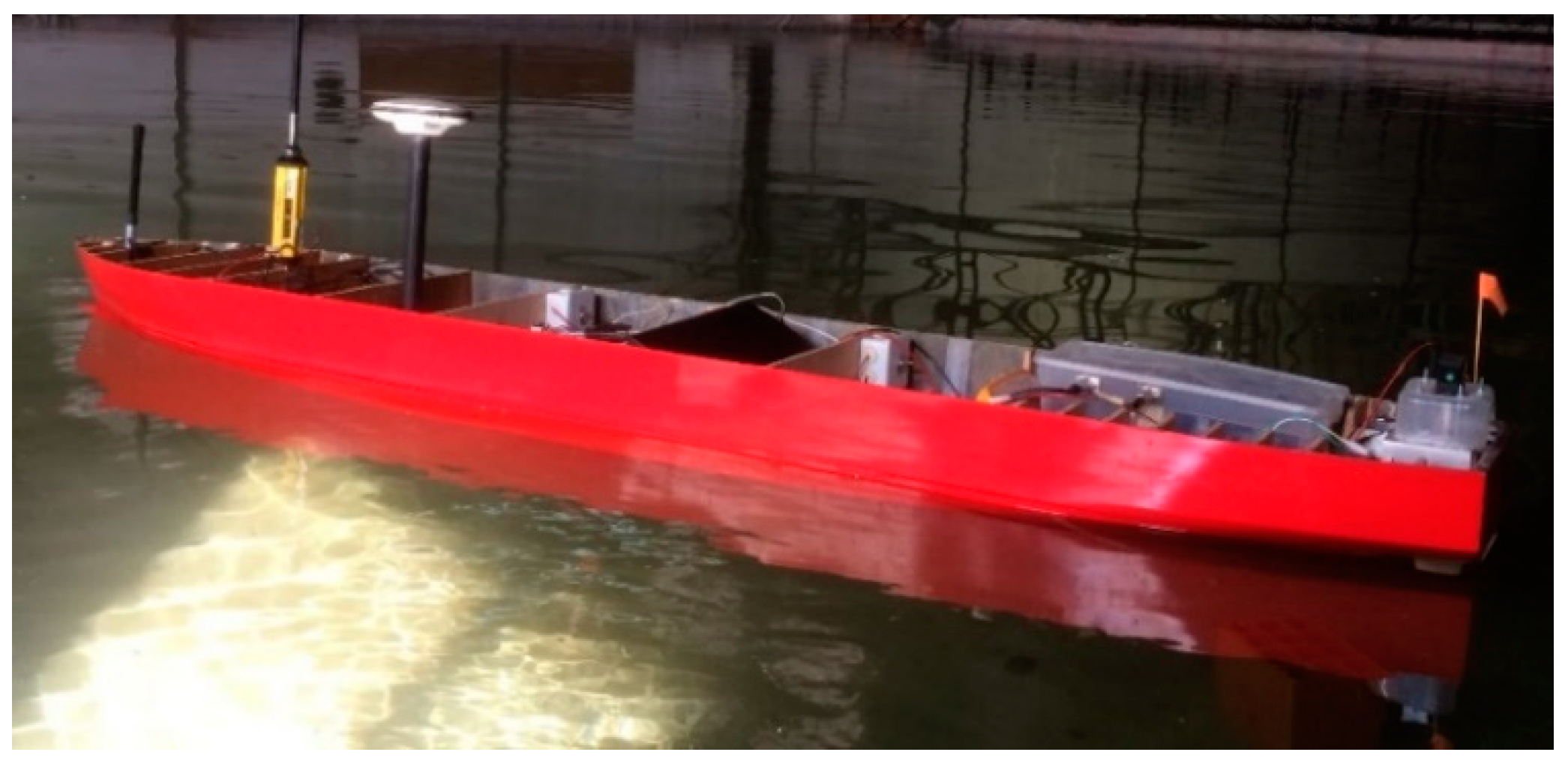
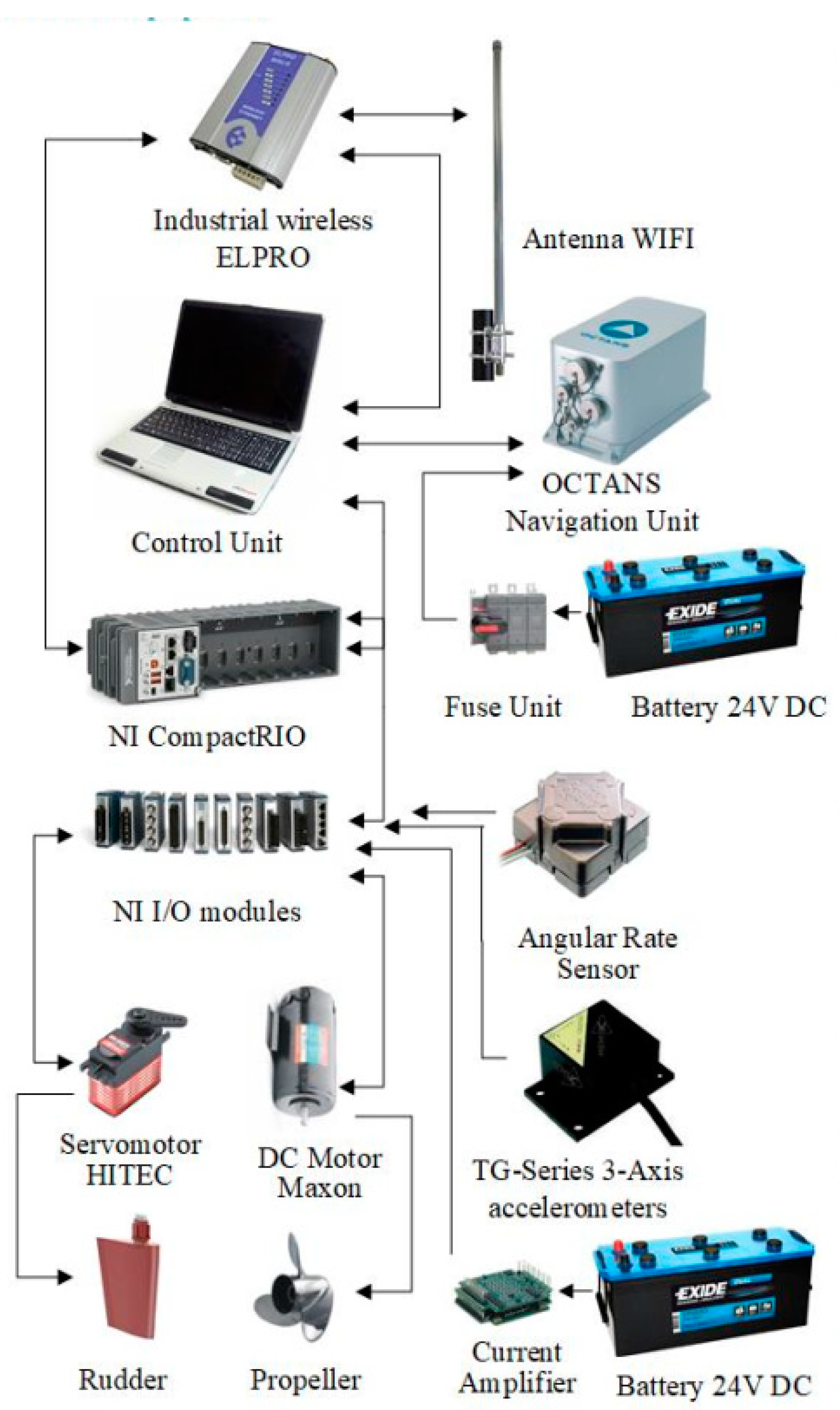
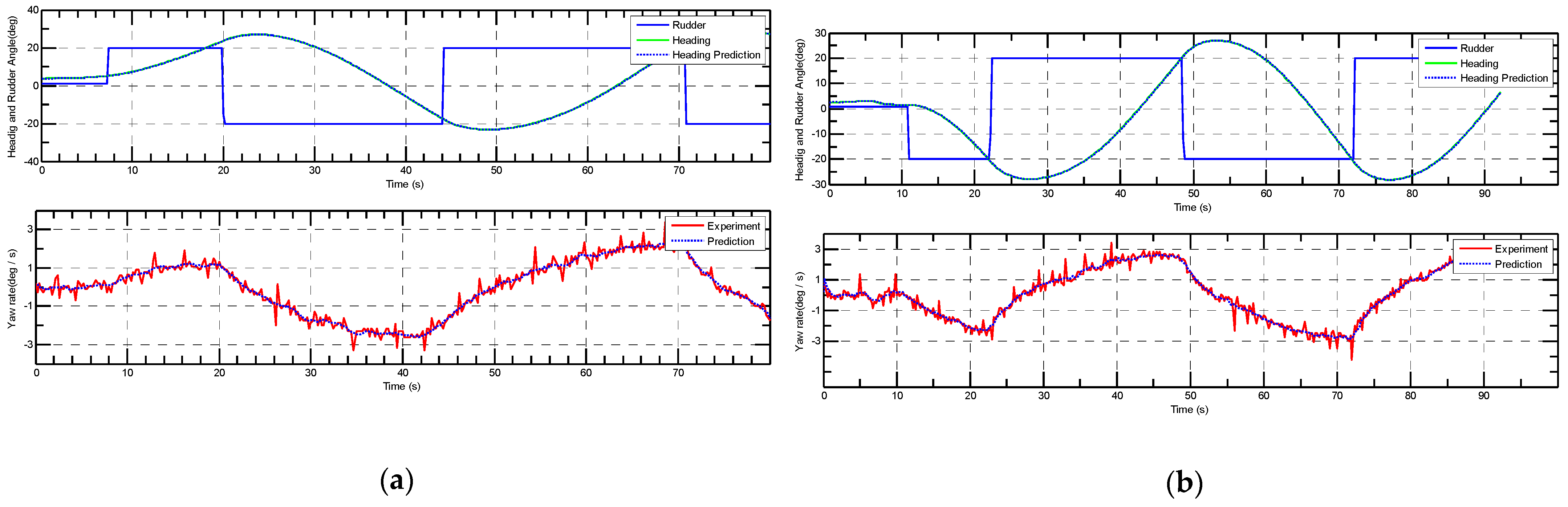
5.1. Nonlinear Manoeuvring Model

A nonlinear manoeuvring model was used in the simulation, which is a modified version of Abkowitz model, and was validated with the manoeuvring tests [55]. The values of the hydrodynamic coefficients can be found in [55]. The time derivatives of u , v and r are given:
{ u ˙ = f 1 m X u ˙ r v ˙ = 1 f 4 [ ( I z N r ˙ ) f 2 ( m x G Y r ˙ ) f 3 ] r ˙ = 1 f 4 [ ( m Y v ˙ r ) f 3 ( m x G N v ˙ r ) f 2 ]
where the nondimensionalized forces and moments are given:
{ f 1 = η 1 u 2 + η 2 n u + η 3 n 2 C R + X v 2 v r 2 + X e 2 e 2 + ( X r 2 + m x G ) r 2 + ( X v r + m ) v r + X v 2 r 2 v 2 r 2 f 2 = Y 0 + { Y v v + Y δ ( c c 0 ) v } + { ( Y r m u ) r Y δ 2 ( c c 0 ) r } + Y δ δ + Y r 2 v r 2 v + Y e 3 e 3 f 3 = N 0 + { N v v N δ ( c c 0 ) v } + { ( N r m x G u ) r + 1 2 N δ ( c c 0 ) r } + N δ δ + N r 2 v r 2 v + N e 3 e 3 f 4 = ( m Y v ˙ ) ( I z N r ˙ ) ( m x G N v ˙ ) ( m x G Y r ˙ )
For the autopilot, the parameters are defined as: Kd = 0.4, η = 1 and λ = 0.1. The time-varying function is chosen as θ ( t , y e ) = 0.4 | y e | + 1 , which renders the system equilibrium point of the guidance subsystem as USGES.

5.2. Single Static Obstacle

In the simulation, one static obstacle near the path is considered. When the obstacle is round, as presented in Figure 10a,b, the deviations are set as, σ x = σ y = 1 . When the obstacle is rectangular, an asymmetric repelling field can be generated by setting the different deviations in the x and y directions, as presented in Figure 10c,d. The deviations of the repelling field can be set as σ x = 2 L p p , σ y = 3 B , where L is the length of the ship and B is the width. The obstacle locates at the same position in both case, p 0 = [ 10 , 5 ] .
The trajectory of the ship in the simulation is given in Figure 10. The blue vectors show the desired heading angle, generated using the repelling function. In Figure 10a, a simulation around static obstacle is given, where the collision risk switches on. The trajectory of the ship is more practical compared with the trajectory in Figure 10b, where the collision risk control was switched off. The obstacle collision avoidance system switches off when the collision risk is zero, which can be observed from the partial enlargement in Figure 10a. When the collision risk control is switched off, as shown in Figure 10b, the obstacle collision avoidance system will push the ship away from the obstacle until it arrives at a safe distance, which is defined by the Gaussian function, as defined in Equations (17) and (18). From Figure 10b, the collision avoidance system without considering the collision risk will inevitably result in some overshoots, which increases fuel consumption. The computational cost and path length are given in Table 1. Obviously, the path length is shorter when considering the collision risk.
The simulation with a rectangular static obstacle near the path is presented in Figure 10c,d. An asymmetric repelling field is used in the simulation. In Figure 10c, the collision risk control is switched on. The resulted trajectory is more reasonable, and the heading angle generated using the repelling vector field is zero when the ship is located outside the velocity obstacle area. The trajectory with a large oscillation is presented in Figure 10d. It results from alternative actions of repelling field and vector field, where repelling field generated the heading angle that pull the ship away from the obstacle, while the vector field provides the opposite effect. As can be observed, the proposed method can control the ship to avoid the obstacles, meanwhile, the path-following task is also an important factor. The traditional obstacle avoidance system usually only emphasizes how to minimize the collision risk [56,57]. Therefore, the collision avoidance methods will take the ship to travel away from obstacles and neglect the path-following task. The proposed method considers both tasks, path-following and obstacle avoidance, at the same time.
In the beginning, the ship travels at a high speed, then the ship will reduce its speed to avoid the obstacles. During the collision avoidance, the ship travels at a constant speed. Figure 11 shows the heading angle and surge speed (desired versus true) in four cases. The ship tracks the desired heading angle, as presented in Figure 11. It demonstrates that the autopilot works well in the simulations. When the collision risk control is switched off, the underactuated surface ship takes a long time to converge to the desired heading angle, which is due to the alternative actions of repelling field and vector field guidance laws. This phenomenon is more obvious in Figure 11d.
Figure 12 presents the rudder angles, cross-track errors in the simulations. The chattering due to the sliding mode control is diminished using the saturation function. The collision risk can reduce the rudder oscillations and have smaller cross-track errors, as presented in Figure 12a,c. In Figure 12b,d, the cross-track errors increase a bit when the ship approaches the obstacle. This is because that the repelling vector field plays a major role in the guidance system, and almost completely cancels the effect of the vector field guidance law.

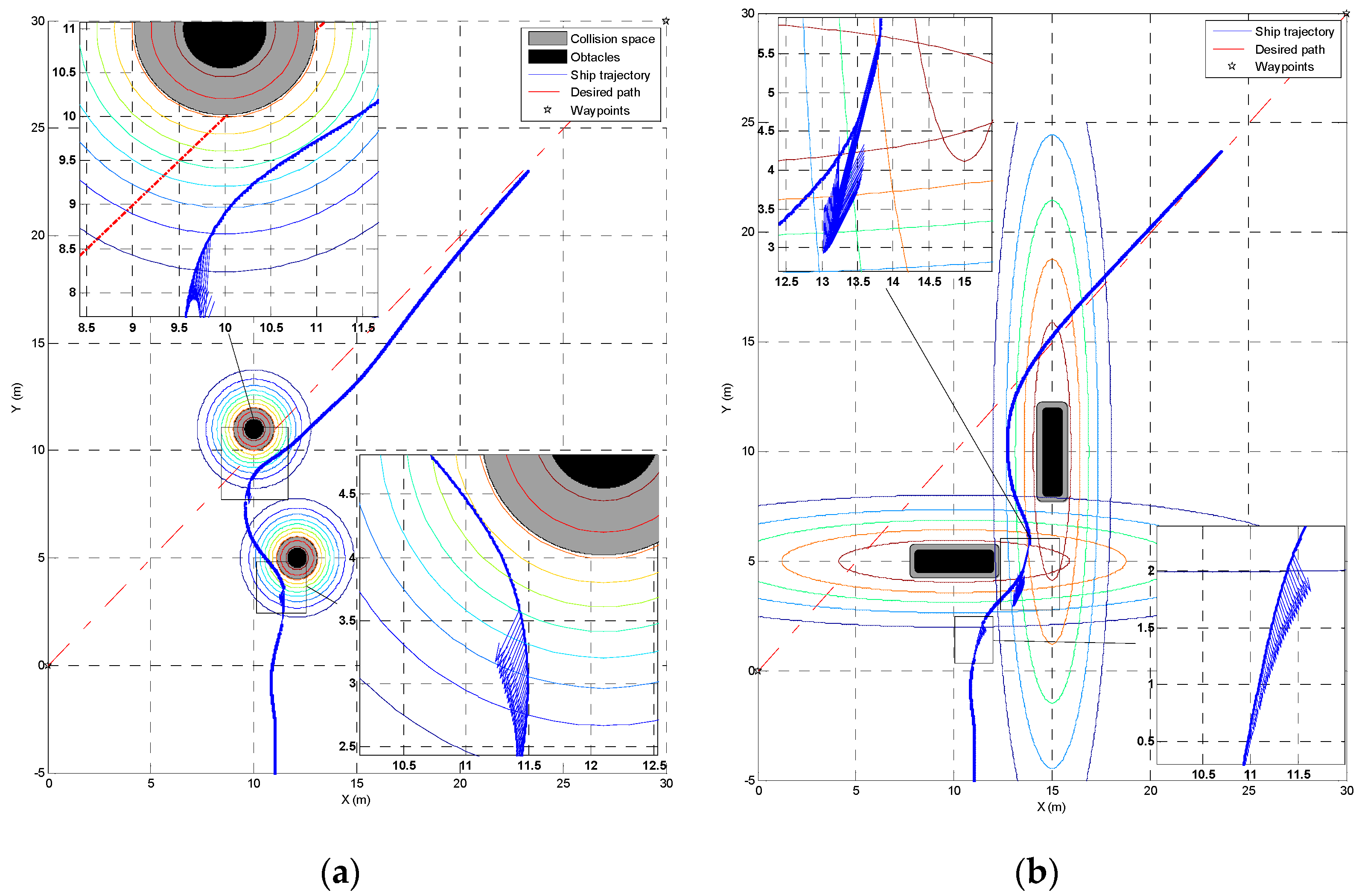
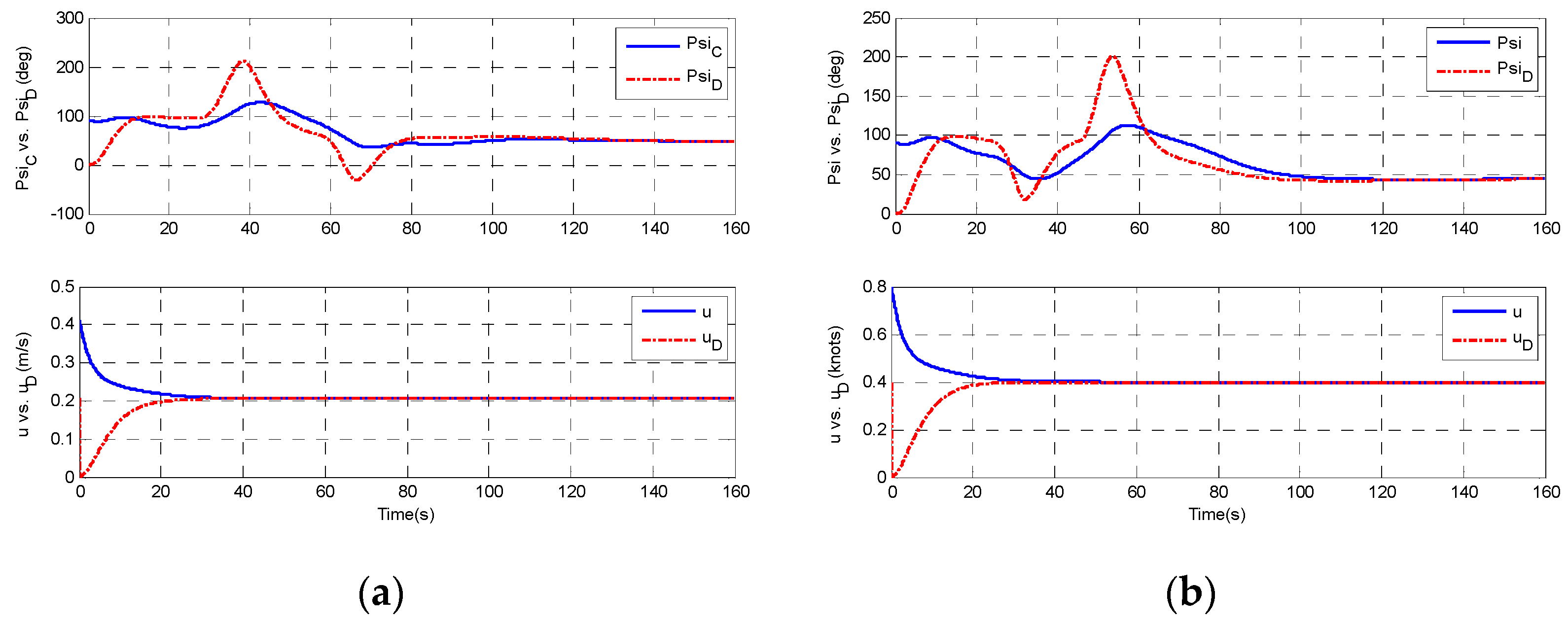
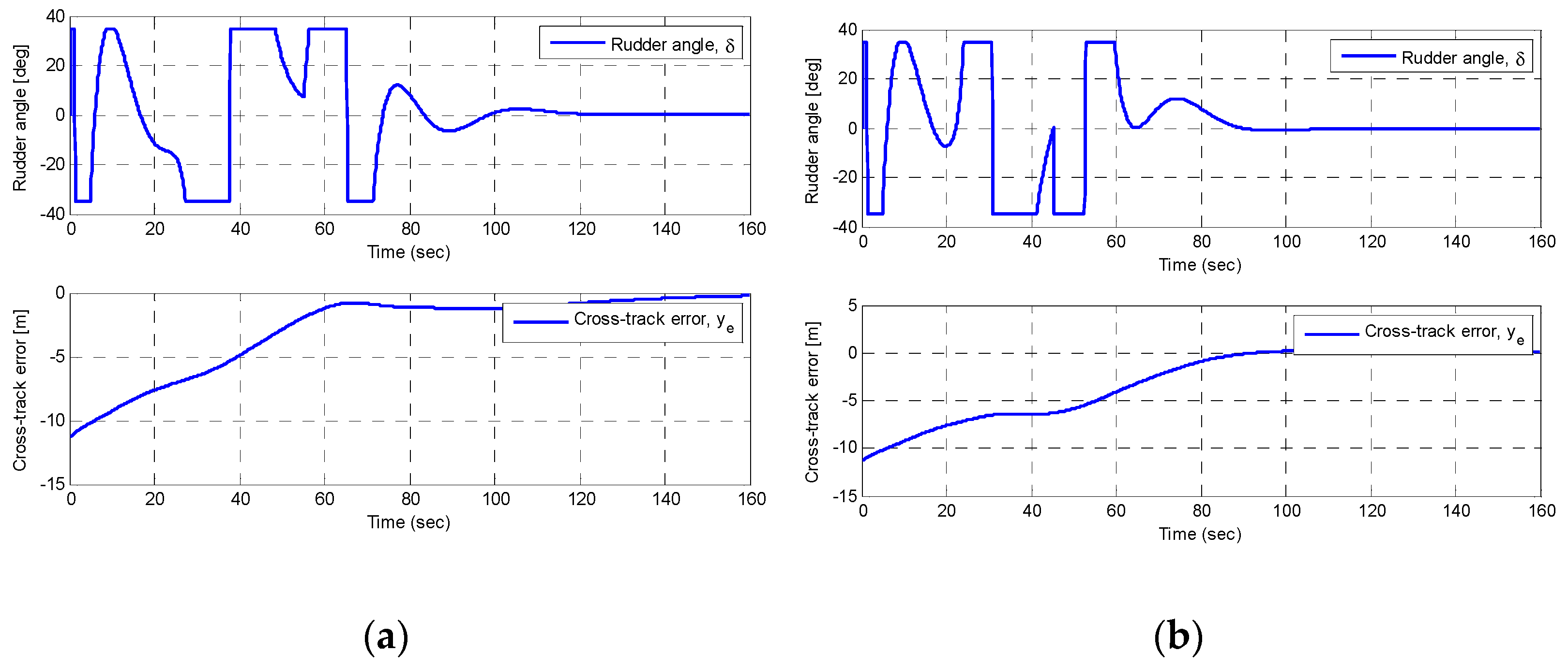
5.3. Multi Static Obstacles

The simulations on path-following and obstacle avoidance control are carried out in the presence of two static obstacles. Both round and rectangular obstacles are considered in the simulations.
The deviations of the repelling function can be chosen from the same values. The positions of the two obstacles in the round case are p 0 = [ 10 , 5 ] and p 1 = [ 15 , 10 ] . The positions of two rectangular obstacles are p 0 = [ 10 , 5 ] and p 1 = [ 25 , 10 ] , respectively. According to the above discussion, collision risk plays an important role in the obstacle collision avoidance system. Therefore, collision risk control was switched on in the following simulation.
Figure 13 shows the trajectories of the ship in the simulations. In Figure 13a, the simulation with two round obstacles is studied. From the partial enlargement of Figure 13, the desired heading angle due to the repelling field is zero when the ship is out of the VO area. In other words, the collision risk of the ship is zero. Only the vector field guidance law will work and the ship will follow the desired heading angle generated by the guidance system. It will converge to the path. When the ship enters the VO area of the second obstacle, the collision risk is nonzero, as presented in Figure 13. The simulation with two rectangular obstacles is presented in Figure 13b. From this Figure, the proposed system can control the ship travelling towards the predefined path and avoid the static obstacles. The computational cost and path length during the simulations are given in Table 2.
Figure 14 shows the heading angle and surge speed in the simulations. The cross-tack error and rudder angle are presented in Figure 15. As can be observed, the rudder angle changes significantly in the second case due to the different shape of the obstacles. The cross-tack errors converge to zero in both cases.

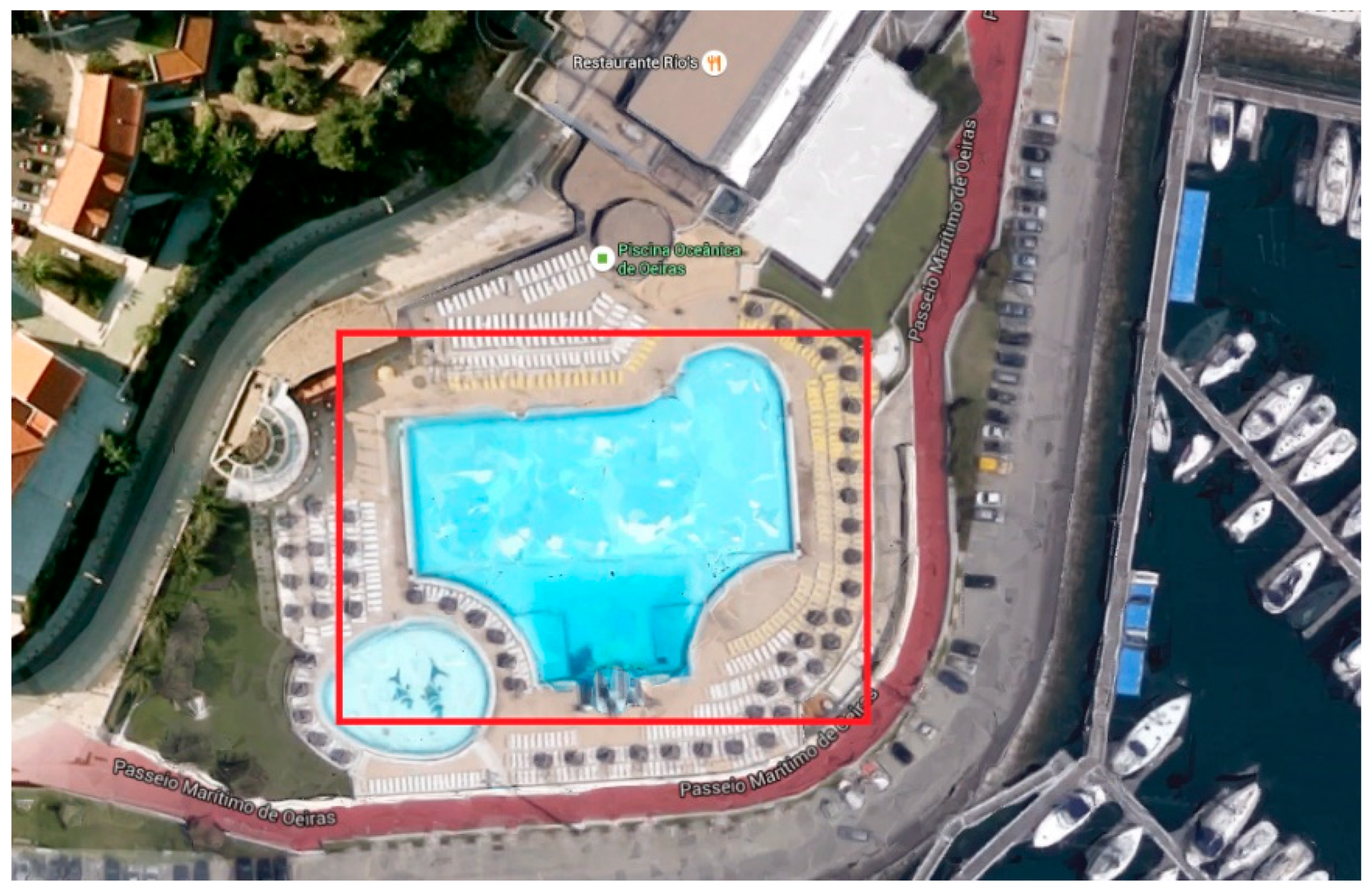
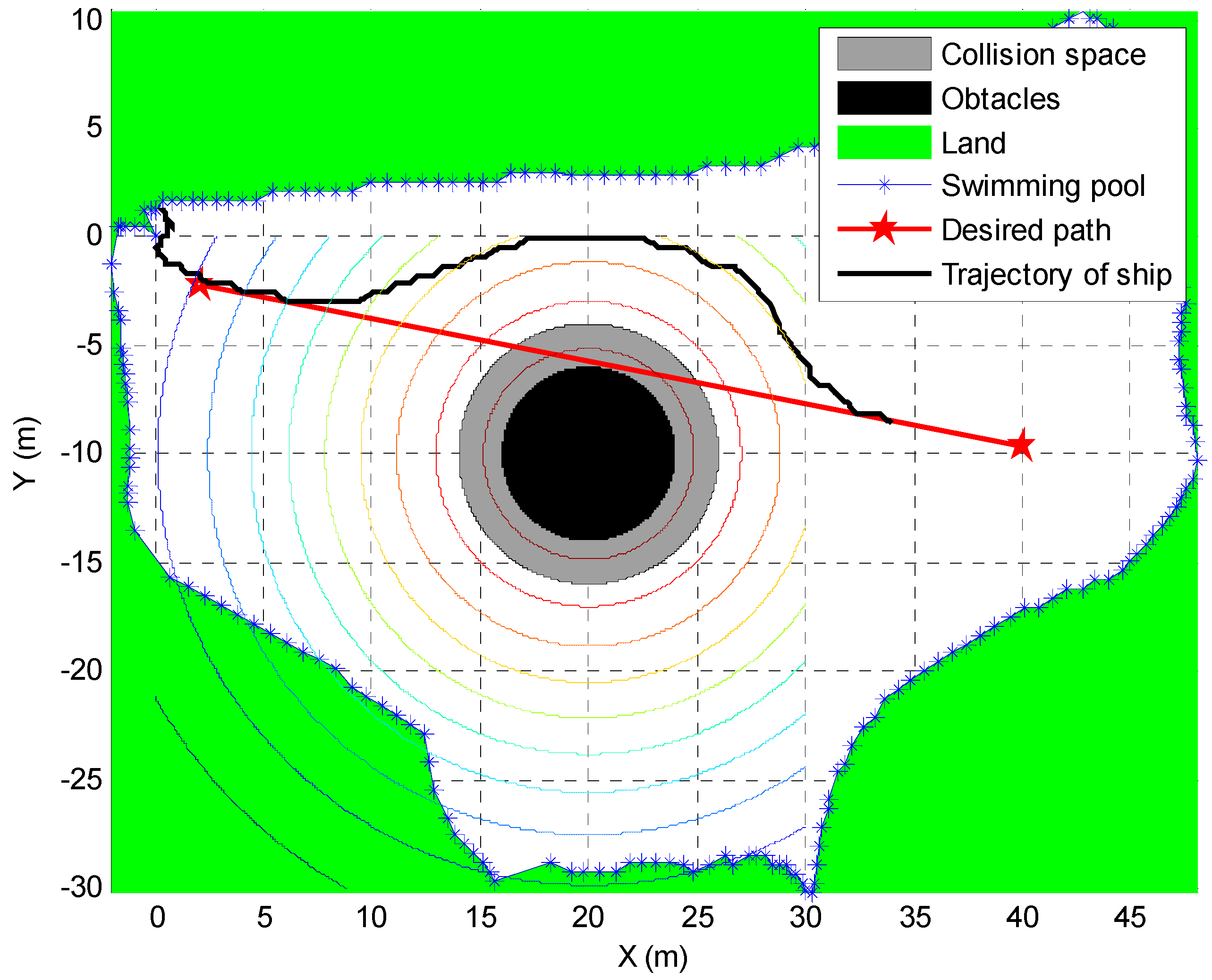
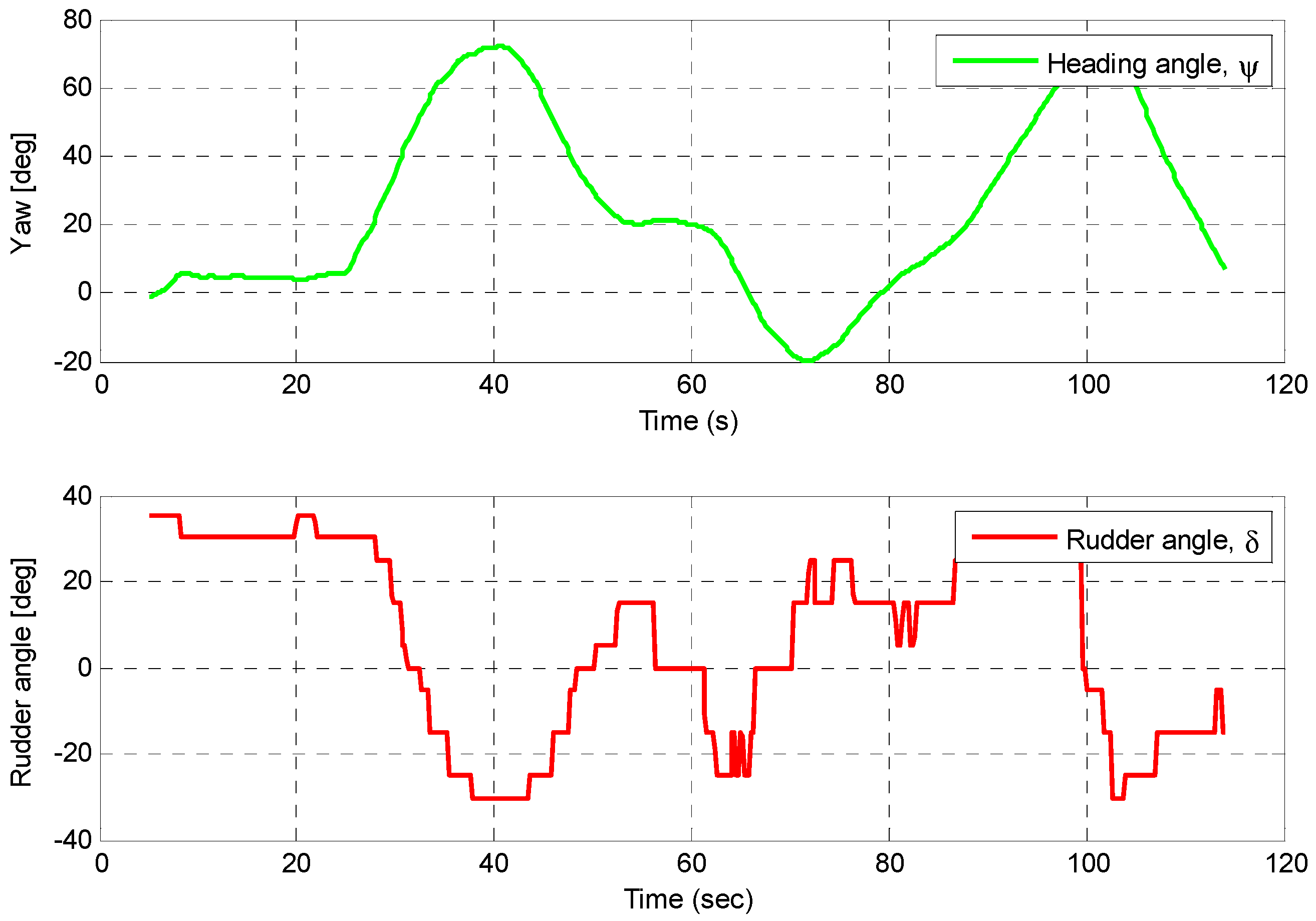
5.4. Collision Avoidance Test Using Ship Model

The collision avoidance test is carried out using a free-running ship model, which was described in Section 2. The sensors and actuators are installed on the ship model, as presented in Figure 4. The control system is programmed in Labview platform. The test was carried out in a swimming pool, as described in Figure 16. The maximum length is 50 m and the width is 20 m, the depth is 1.2–1.8 m.
The path-following and collision avoidance were carried out using a scaled marine surface ship model. Here, only one obstacle was considered due to the limited geometry dimension of the swimming pool. The obstacle was assumed to be located in the middle of the swimming pool. The ship will travel from the northeast to the southwest corner of the swimming pool. Before tests, the battery was charged fully, and the draft of the ship model was adjusted to the designed value. The rudder and propeller were checked and tested in manual operation. The sensors were initiated and were calibrated to zero, such as the Differential Global Positioning System (DGPS), inertial measurement unit (IMU), and wind sensor. During the model tests, the revolutions per minute (RPM) was set as constant. At the beginning of the tests, the ship model was released with zero rudder angle and constant RPM. If the ship cannot go straight, it is necessary to change the position of the weights in the ship model.
The static obstacle is located at p 0 = [ 20 , 10 ] , as indicated in black colour. The diameter is 6 m and the deviations are set as σ x = σ y = 4 * L p p . Figure 17 presents the trajectories of the ship model in the test. Considering the safety, it is better to set a larger variance of the repelling function, because of the environmental disturbance, for example, the wind and wave are large for a scaled ship model. As shown in the Figure, the collision avoidance method can control the underactuated ship model to avoid the collision. Figure 18 shows the heading angle and rudder angle during the test. The initial heading angle is set to zero. From the figure, the heading angle approaches zero when the ship passes the obstacle.

6. Conclusions

This paper proposes an integrated path-following and risk-based obstacle collision avoidance system using the vector field method for underactuated autonomous surface vehicles. It is different from the obstacle avoidance methods in most published papers, which usually treat the path-following and obstacle collision avoidance separately. This paper considers the coupled path following and collision avoidance task. Meanwhile, the stability of the guidance and control system was analysed using the Lyapunov stability theory. For the control system, a sliding mode control was designed based on a nonlinear steering model. To obtain the steering model, the manoeuvring tests were carried out using a free-running ship model, and the collected data were used to estimate the values of the parameters using the LS-SVM. The equilibrium point of the heading error dynamic equations is GES. For the guidance system, the vector field guidance law was used and the stability proof of USGES was given. To avoid the obstacle near the path, the proposed guidance law was extended using a repelling function. The resulting heading angle can control the ship’s travel away from the obstacles, which meanwhile, is converging to the predefined path when the collision risk is zero. Simulations and model tests were carried out to test the integrated system. From the simulation tests, it can be concluded that the collision risk plays an important role in the system. It can avoid the overshoot in collision avoidance, and the resulting trajectory of the underactuated ship model is more practical. Considering the expensive cost of testing on a full-scale ship, the proposed system was only validated using a scaled ship model. The test shows that the ship model can follow the predefined path and avoid colliding with the obstacles. In the future, the parameters of the proposed system can be optimized based on the specified task or environmental disturbance. More model tests in large areas with more complex environmental disturbance, such as dynamic obstacle, wind, waves, can be carried out for validation.

Author Contributions

Conceptualization, H.X. and C.G.S.; methodology, H.X. and C.G.S.; software, H.X. and M.A.H.; validation, H.X. and M.A.H.; formal analysis, H.X.; investigation, H.X.; resources, H.X.; data curation, H.X. and M.A.H.; writing—original draft preparation, H.X.; writing—review and editing, H.X., M.A.H. and C.G.S.; visualization, H.X.; supervision, C.G.S.; project administration, C.G.S.; funding acquisition, C.G.S. All authors have read and agreed to the published version of the manuscript.

Funding

This research was supported by the Portuguese Foundation for Science and Technology (Fundação para a Ciência e Tecnologia–FCT) under grants for the ROUTING research project (MARTERA-1/ROUTING/3/2018) in the ERA-NET COFUND MarTERA-1 programme (2018–2021). This work was performed within the Strategic Research Plan of the Centre for Marine Technology and Ocean Engineering, financed by the Portuguese Foundation for Science and Technology (Fundação para a Ciência e Tecnologia-FCT) under contract UIDB/UIDP/00134/2020.

Institutional Review Board Statement

This study does not involve humans or animals.

Informed Consent Statement

Not applicable.

Data Availability Statement

Not applicable.

Conflicts of Interest

The authors declare that they have no conflict of interest.

References

  1. Guedes Soares, C.; Teixeira, A.P. Risk Assessment in Maritime Transportation. Reliab. Eng. Syst. Saf. 2001, 74, 299–309. [Google Scholar] [CrossRef]
  2. Allianz Global Corporate and Speciality. Safety and Shipping Review 2018; Allianz Global Corporate & Specialty: Munich, Germany, 2018. [Google Scholar]
  3. Breivik, M.; Fossen, T.I. Path Following for Marine Surface Vessels. In Oceans ’04 MTS/IEEE Techno-Ocean ’04 (IEEE Cat. No.04CH37600); IEEE: Piscataway, NJ, USA, 2004; Volume 4, pp. 2282–2289. [Google Scholar] [CrossRef]
  4. Breivik, M.; Hovstein, V.E.; Fossen, T.I. Straight-Line Target Tracking for Unmanned Surface Vehicles. Model. Identif. Control A Nor. Res. Bull. 2008, 29, 131–149. [Google Scholar] [CrossRef] [Green Version]
  5. Yanushevsky, R. Guidance of Unmanned Aerial Vehicles; Taylor & Francis: Boca Raton, FL, USA, 2011. [Google Scholar]
  6. Fossen, T.I. Handbook of Marine Craft Hydrodynamics and Motion Control; John Wiley & Sons, Ltd: Chichester, UK, 2011. [Google Scholar] [CrossRef]
  7. Fossen, T.I.; Pettersen, K.Y.; Galeazzi, R. Line-of-Sight Path Following for Dubins Paths with Adaptive Sideslip Compensation of Drift Forces. IEEE Trans. Control Syst. Technol. 2015, 23, 820–827. [Google Scholar] [CrossRef] [Green Version]
  8. Liu, C.; Sun, J.; Zou, Z. Integrated Line of Sight and Model Predictive Control for Path Following and Roll Motion Control Using Rudder. J. Sh. Res. 2015, 59, 99–112. [Google Scholar] [CrossRef]
  9. Fossen, T.I.; Sagatun, S.I.; Sørensen, A.J. Identification of Dynamically Positioned Ships. Model. Identif. Control 1996, 17, 153–165. [Google Scholar] [CrossRef] [Green Version]
  10. Moe, S.; Pettersen, K.Y.; Fossen, T.I.; Gravdahl, J.T. Line-of-Sight Curved Path Following for Underactuated USVs and AUVs in the Horizontal Plane under the Influence of Ocean Currents. In Proceedings of the 24th Mediterranean Conference on Control and Automation, MED 2016, Athens, Greece, 21–24 June 2016; pp. 38–45. [Google Scholar] [CrossRef] [Green Version]
  11. Moe, S.; Pettersen, K.Y. Set-Based Line-of-Sight (LOS) Path Following with Collision Avoidance for Underactuated Unmanned Surface Vessel. In Proceedings of the 24th Mediterranean Conference on Control and Automation, MED 2016, Athens, Greece, 21–24 June 2016; pp. 402–409. [Google Scholar] [CrossRef] [Green Version]
  12. Kelasidi, E.; Liljeback, P.; Pettersen, K.Y.; Gravdahl, J.T. Integral Line-of-Sight Guidance for Path Following Control of Underwater Snake Robots: Theory and Experiments. IEEE Trans. Robot. 2017, 33, 610–628. [Google Scholar] [CrossRef] [Green Version]
  13. Xu, H.; Guedes Soares, C. An Optimized Energy-Efficient Path Following Algorithm for Underactuated Marine Surface Ship Model. Int. J. Marit. Eng. 2018, 160, A-411–A-421. [Google Scholar] [CrossRef]
  14. Lekkas, A.M.; Fossen, T.I. A Time-Varying Lookahead Distance Guidance Law for Path Following. IFAC Proc. Vol. 2012, 9, 398–403. [Google Scholar] [CrossRef] [Green Version]
  15. Moreira, L.; Fossen, T.I.; Guedes Soares, C. Path Following Control System for a Tanker Ship Model. Ocean Eng. 2007, 34, 2074–2085. [Google Scholar] [CrossRef]
  16. Vu, M.T.; Le, T.-H.; Thanh, H.L.N.N.; Huynh, T.-T.; Van, M.; Hoang, Q.-D.; Do, T.D. Robust Position Control of an Over-actuated Underwater Vehicle under Model Uncertainties and Ocean Current Effects Using Dynamic Sliding Mode Surface and Optimal Allocation Control. Sensors 2021, 21, 747. [Google Scholar] [CrossRef]
  17. Vu, M.T.; Le Thanh, H.N.N.; Huynh, T.T.; Thang, Q.; Duc, T.; Hoang, Q.D.; Le, T.H. Station-Keeping Control of a Hovering Over-Actuated Autonomous Underwater Vehicle under Ocean Current Effects and Model Uncertainties in Horizontal Plane. IEEE Access 2021, 9, 6855–6867. [Google Scholar] [CrossRef]
  18. Borhaug, E.; Pavlov, A.; Pettersen, K.Y. Integral LOS Control for Path Following of Underactuated Marine Surface Vessels in the Presence of Constant Ocean Currents. In Proceedings of the 2008 47th IEEE Conference on Decision and Control, Cancun, Mexico, 9–11 December 2008; IEEE: Piscataway, NJ, USA, 2008; pp. 4984–4991. [Google Scholar] [CrossRef] [Green Version]
  19. Caharija, W.; Candeloro, M.; Pettersen, K.Y.; Sørensen, A.J. Relative Velocity Control and Integral Los for Path Following of Underactuated Surface Vessels. IFAC Proc. Vol. 2012, 9, 380–385. [Google Scholar] [CrossRef] [Green Version]
  20. Lekkas, A.M.; Fossen, T.I. Integral LOS Path Following for Curved Paths Based on a Monotone Cubic Hermite Spline Parametrization. IEEE Trans. Control Syst. Technol. 2014, 22, 2287–2301. [Google Scholar] [CrossRef]
  21. Caharija, W.; Pettersen, K.Y.; Bibuli, M.; Calado, P.; Zereik, E.; Braga, J.; Gravdahl, J.T.; Sorensen, A.J.; Milovanovic, M.; Bruzzone, G. Integral Line-of-Sight Guidance and Control of Underactuated Marine Vehicles: Theory, Simulations, and Experiments. IEEE Trans. Control Syst. Technol. 2016, 24, 1623–1642. [Google Scholar] [CrossRef] [Green Version]
  22. Fossen, T.I.; Lekkas, A.M. Direct and Indirect Adaptive Integral Line-of-Sight Path-Following Controllers for Marine Craft Exposed to Ocean Currents. Int. J. Adapt. Control Signal Process. 2015, 31, 445–463. [Google Scholar] [CrossRef]
  23. Nelson, D.R.; Barber, D.B.; McLain, T.W.; Beard, R.W. Vector Field Path Following for Small Unmanned Air Vehicles. In Proceedings of the 2006 American Control Conference, Minneapolis, MN, USA, 14–16 June 2006; pp. 5788–5794. [Google Scholar] [CrossRef]
  24. Nelson, D.R.; Barber, D.B.; McLain, T.W.; Beard, R.W. Vector Field Path Following for Miniature Air Vehicles. IEEE Trans. Robot. 2007, 23, 519–529. [Google Scholar] [CrossRef] [Green Version]
  25. Lawrence, D.A.; Frew, E.W.; Pisano, W.J. Lyapunov Vector Fields for Autonomous Unmanned Aircraft Flight Control. J. Guid. Control. Dyn. 2008, 31, 1220–1229. [Google Scholar] [CrossRef]
  26. Wang, Y.; Wang, X.; Zhao, S.; Shen, L. Vector Field Based Sliding Mode Control of Curved Path Following for Miniature Unmanned Aerial Vehicles in Winds. J. Syst. Sci. Complex. 2018, 31, 302–324. [Google Scholar] [CrossRef]
  27. Xu, H.; Guedes Soares, C. Vector Field Path Following for Surface Marine Vessel and Parameter Identification Based on LS-SVM. Ocean Eng. 2016, 113, 151–161. [Google Scholar] [CrossRef]
  28. Xu, H.T.; Guedes Soares, C. Waypoint-Following for a Marine Surface Ship Model Based on Vector Field Guidance Law. In Maritime Technology and Engineering 3; Guedes Soares, C., Santos, T.A., Eds.; Taylor & Francis Group: London, UK, 2016; Volume 1, pp. 409–418. [Google Scholar]
  29. Caharija, W.; Pettersen, K.Y.; Calado, P.; Braga, J. A Comparison between the ILOS Guidance and the Vector Field Guidance. IFAC-PapersOnLine 2015, 28, 89–94. [Google Scholar] [CrossRef]
  30. Khalil, H.K. Nonlinear Systems, 3rd ed.; Prentice Hall: Upper Saddle River, NJ, USA, 2002. [Google Scholar]
  31. Loría, A.; Panteley, E. Cascaded Nonlinear Time-Varying Systems: Analysis and Design. In Advanced Topics in Control Systems Theory: Lecture Notes from FAP 2004; Lamnabhi-Lagarrigue, F., Loría, A., Panteley, E., Eds.; Springer: London, UK, 2005; pp. 23–64. [Google Scholar] [CrossRef]
  32. Fossen, T.I.; Pettersen, K.Y. On Uniform Semiglobal Exponential Stability (USGES) of Proportional Line-of-Sight Guidance Laws. Automatica 2014, 50, 2912–2917. [Google Scholar] [CrossRef] [Green Version]
  33. Borhaug, E.; Pettersen, K.Y. Cross-Track Control for Underactuated Autonomous Vehicles. In Proceedings of the 44th IEEE Conference on Decision and Control, Seville, Spain, 15 December 2005; IEEE: Piscataway, NJ, USA, 2005; Volume 2005, pp. 602–608. [Google Scholar] [CrossRef]
  34. Fredriksen, E.; Pettersen, K.Y. Global κ-Exponential Way-Point Maneuvering of Ships: Theory and Experiments. Automatica 2006, 42, 677–687. [Google Scholar] [CrossRef]
  35. Beard, R.W.; McLain, T.W. Small Unmanned Aircraft: Theory and Practice; Princeton University Press: Princeton, NJ, USA, 2013. [Google Scholar] [CrossRef]
  36. Zhang, J.; Zhang, D.; Yan, X.; Haugen, S.; Guedes Soares, C. A Distributed Anti-Collision Decision Support Formulation in Multi-Ship Encounter Situations under COLREGs. Ocean Eng. 2015. [Google Scholar] [CrossRef]
  37. Perera, L.P.; Moreira, L.; Santos, F.P.; Ferrari, V.; Sutulo, S.; Guedes Soares, C. A Navigation and Control Platform for Real-Time Manoeuvring of Autonomous Ship Models. IFAC Proc. Vol. 2012, 9, 465–470. [Google Scholar] [CrossRef]
  38. Perera, L.P.; Carvalho, J.P.; Guedes Soares, C. Fuzzy Logic Based Decision Making System for Collision Avoidance of Ocean Navigation under Critical Collision Conditions. J. Mar. Sci. Technol. 2011, 16, 84–99. [Google Scholar] [CrossRef]
  39. Perera, L.P.; Ferrari, V.; Santos, F.P.; Hinostroza, M.A.; Guedes Soares, C. Experimental Evaluations on Ship Autonomous Navigation and Collision Avoidance by Intelligent Guidance. IEEE J. Ocean. Eng. 2015, 40, 374–387. [Google Scholar] [CrossRef]
  40. Statheros, T.; Howells, G.; Maier, K.M. Autonomous Ship Collision Avoidance Navigation Concepts, Technologies and Techniques. J. Navig. 2008, 61, 129–142. [Google Scholar] [CrossRef] [Green Version]
  41. Huang, Y.; van Gelder, P.H.A.J.M.; Wen, Y. Velocity Obstacle Algorithms for Collision Prevention at Sea. Ocean Eng. 2018, 151, 308–321. [Google Scholar] [CrossRef]
  42. Huang, Y.; Chen, L.; van Gelder, P.H.A.J.M. Generalized Velocity Obstacle Algorithm for Preventing Ship Collisions at Sea. Ocean Eng. 2019, 173, 142–156. [Google Scholar] [CrossRef]
  43. Kuwata, Y.; Wolf, M.T.; Zarzhitsky, D.; Huntsberger, T.L. Safe Maritime Autonomous Navigation with COLREGS, Using Velocity Obstacles. IEEE J. Ocean. Eng. 2014, 39, 110–119. [Google Scholar] [CrossRef]
  44. Mou, J.M.; van der Tak, C.; Ligteringen, H. Study on Collision Avoidance in Busy Waterways by Using AIS Data. Ocean Eng. 2010, 37, 483–490. [Google Scholar] [CrossRef]
  45. Vu, M.T.; Van, M.; Bui, D.H.P.; Do, Q.T.; Huynh, T.-T.; Lee, S.D.; Choi, H.S. Study on Dynamic Behavior of Unmanned Surface Vehicle-Linked Unmanned Underwater Vehicle System for Underwater Exploration. Sensors 2020, 20, 1329. [Google Scholar] [CrossRef] [PubMed] [Green Version]
  46. Sutulo, S.; Guedes Soares, C. Mathematical Models for Simulation of Manoeuvring Performance of Ships. In Maritime Engineering and Technology; Guedes Soares, C., Garbatov, Y., Fonseca, N., Teixeira, A.P., Eds.; Taylor & Francis Group: London, UK, 2011; pp. 661–698. [Google Scholar]
  47. Xu, H.; Hassani, V.; Hinostroza, M.A.; Guedes Soares, C. Real-Time Parameter Estimation of Nonlinear Vessel Steering Model Using Support Vector Machine. In Proceedings of the ASME 2018 37th International Conference on Ocean, Offshore and Arctic Engineering, Madrid, Spain, 17–22 June 2018; ASME: Madrid, Spain, 2018. [Google Scholar] [CrossRef] [Green Version]
  48. Xu, H.; Fossen, T.I.; Guedes Soares, C. Uniformly Semiglobally Exponential Stability of Vector Field Guidance Law and Autopilot for Path-Following. Eur. J. Control 2020, 53, 88–97. [Google Scholar] [CrossRef]
  49. ITTC. Recommended Procedures and Guidelines: Free Running Model Tests. In Proceedings of the 23rd International Towing Tank Conference, Venice, Italy, 8–14 September 2002. [Google Scholar]
  50. Xu, H.; Guedes Soares, C. Hydrodynamic Coefficient Estimation for Ship Manoeuvring in Shallow Water Using an Optimal Truncated LS-SVM. Ocean Eng. 2019, 191, 106488. [Google Scholar] [CrossRef]
  51. Xu, H.; Guedes Soares, C. Manoeuvring Modelling of a Containership in Shallow Water Based on Optimal Truncated Nonlinear Kernel-Based Least Square Support Vector Machine and Quantum-Inspired Evolutionary Algorithm. Ocean Eng. 2020, 195, 106676. [Google Scholar] [CrossRef]
  52. Xu, H.T.; Oliveira, P.; Guedes Soares, C. L1 adaptive backstepping control for path-following of underactuated marine surface ship. Eur. J. Control 2021, 58, 357–372. [Google Scholar] [CrossRef]
  53. Szlapczynski, R.; Szlapczynska, J. Review of Ship Safety Domains: Models and Applications. Ocean Eng. 2017, 145, 277–289. [Google Scholar] [CrossRef]
  54. Guy, S.J.; Chhugani, J.; Kim, C.; Satish, N.; Lin, M.; Manocha, D.; Dubey, P. ClearPath: Highly Parallel Collision Avoidance for Multi-Agent Simulation. In Proceedings of the 2009 ACM SIGGRAPH/Eurographics Symposium on Computer Animation-SCA ’09, Los Angeles, CA, USA, 7–9 August 2015; ACM Press: New York, NY, USA, 2009; pp. 177–187. [Google Scholar] [CrossRef]
  55. Xu, H.; Hinostroza, M.A.; Guedes Soares, C. Estimation of Hydrodynamic Coefficients of a Nonlinear Manoeuvring Mathematical Model with Free-Running Ship Model Tests. Int. J. Marit. Eng. 2018, 160, A-213–A-226. [Google Scholar] [CrossRef]
  56. Silveira, P.A.M.; Teixeira, A.P.; Guedes Soares, C. Use of AIS Data to Characterise Marine Traffic Patterns and Ship Collision Risk off the Coast of Portugal. J. Navig. 2013. [Google Scholar] [CrossRef] [Green Version]
  57. Perera, L.P.; Oliveira, P.; Guedes Soares, C. System Identification of Nonlinear Vessel Steering. J. Offshore Mech. Arct. Eng. 2015, 137, 031302. [Google Scholar] [CrossRef] [Green Version]
Figure 1. The block diagrams of path-following control for marine ships.
Jmse 09 00652 g001
Figure 2. Geometry description of path-following control.
Jmse 09 00652 g002
Figure 3. A scaled free-running chemical tanker.
Jmse 09 00652 g003
Figure 4. Sensors and actuators used in the free-running ship model.
Jmse 09 00652 g004
Figure 5. LS-SVM for parameter estimation using 20°−20° zigzag manoeuvring tests: (a) training result; and (b) validation.
Jmse 09 00652 g005
Figure 6. Vector space around the predefined path (red line).
Jmse 09 00652 g006
Figure 7. The proposed collision avoidance system for autonomous surface ships ((a): geometry chart; and (b): the flowchart).
Jmse 09 00652 g007
Figure 8. The velocity obstacle (VO) with a static obstacle. The green area represents the obstacle. The area surrounded by a dotted elliptical line is the obstacle domain. The area surrounded by a red elliptical line is the conflict position (ConfP).
Jmse 09 00652 g008
Figure 9. Illustration of the velocity obstacle (VO) regions.
Jmse 09 00652 g009
Figure 10. Trajectory of the underactuated ship: (a) round obstacle with collision risk; (b) round obstacle without collision risk; (c) rectangular obstacle with collision risk; and (d) rectangular obstacle without collision risk.
Jmse 09 00652 g010
Figure 11. Heading angle, surge speed (desired versus true) from the simulations: (a) round obstacle with collision risk; (b) round obstacle without collision risk; (c) rectangular obstacle with collision risk; and (d) rectangular obstacle without collision risk.
Jmse 09 00652 g011
Figure 12. Rudder angle, cross-track error from the simulations: (a) round obstacle with collision risk; (b): round obstacle without collision risk; and (c) rectangular obstacle with collision risk; (d): rectangular obstacle without collision risk.
Jmse 09 00652 g012
Figure 13. Path-following simulation with multi static obstacles: (a) round obstacles; and (b) rectangular obstacles.
Jmse 09 00652 g013
Figure 14. Heading angle, surge speed (desired versus true): (a) multi round obstacle; and (b) multi rectangular obstacle.
Jmse 09 00652 g014
Figure 15. Rudder angle, cross-track errors: (a) multi round obstacle; and (b) multi rectangular obstacle.
Jmse 09 00652 g015
Figure 16. Location of the collision avoidance test.
Jmse 09 00652 g016
Figure 17. The path following and collision avoidance test using a free-running ship model.
Jmse 09 00652 g017
Figure 18. Heading angle and rudder angle during the test.
Jmse 09 00652 g018
Table 1. The computational cost and path length in the simulations with a single obstacle.
Test aTest bTest cTest d
Path length (m)29.14223.64826.95048.820
Computational cost (s)1.7381.3101.3242.167
Table 2. The computational cost and path length in the simulations with multi static obstacles.
Test aTest b
Path length (m)34.07534.576
Computational cost (s)1.4741.516
Publisher’s Note: MDPI stays neutral with regard to jurisdictional claims in published maps and institutional affiliations.

