Towfish Attitude Control: A Consideration of Towing Point, Center of Gravity, and Towing Speed

Abstract

This paper deals with the attitude control of a towfish (underwater towed vehicle) with two elevators and a single rudder to improve the image quality of an attached sound navigation ranging (sonar) system. Image distortion can occur if the towfish shakes excessively. Since a towfish is connected to the mother ship through a towing cable and the motion of the towfish is affected not only by the motion of the cable, but also by the position of the center of gravity, towing point, and towing speed, it is necessary to analyze how these factors affect the towfish to appropriately control its attitude. In this study, a method for obtaining a feasible region of the towing point in accordance with the variations in the center of gravity and towing speed is proposed, and the feasible region obtained can ensure that pitch control can be achieved using the installed elevators. In addition, the allowable range of disturbances for yaw control was also investigated. Simulations were conducted using the dynamic models of the towfish and cable to check the obtained feasible region/range, and it was confirmed that there is a region/range where the attitude control can be carried out with relative ease.

1. Introduction

Unmanned underwater vehicles (UUVs) are frequently used for marine environmental data collection, submarine topography mapping, and military purposes, among other uses [1]. Autonomous underwater vehicles (AUVs) and towfish (underwater towed vehicles) are widely used. An AUV has the advantage of being able to move freely and can operate autonomously without operator intervention [2,3,4]; however, the power supply is limited, making it difficult to apply for long-term missions [5,6]. By contrast, the towfish is connected to the mother ship through the towing cable and its motion is constrained; however, the observation data can be transmitted to the mother ship in real-time, and the power is supplied by the mother ship continuously, allowing real-time, long-term, and wide-area observations [7,8,9]. We are currently developing a towfish with a sonar system, and this paper deals with its attitude control to improve the quality of the sonar image.

The towfish is usually designed to be stable in movement; however, it is difficult to fully respond to unpredictable underwater environments and various operating conditions. In particular, if an interferometric synthetic aperture sonar (InSAS) with 10-times the resolution of the existing side scan sonar (SSS) is mounted onto the towfish, the irregular motion of the towfish causes distortion or defocusing of the InSAS image [10]. Thus, precise attitude control is required to improve the image quality.

Related studies on towed vehicles for various purposes can be found [11,12,13,14,15,16,17,18,19,20,21,22,23,24,25,26,27,28]. Research on improving the image of a sonar system mounted on a towfish [11,12,13] and obstacle avoidance for route tracking [14,15,16,17,18] were conducted. In addition, depth and attitude control using various controllers were studied [19,20,21,22,23,24,25,26]. Moreover, the vertical and horizontal shaking of a towed vehicle for monitoring submarine pipeline conditions [27] and turn maneuvering [28] are discussed. These studies are mainly focused aspects of the control method; however, the towfish is affected by various factors such as the towing point, position of the center of gravity, and towing speed. This paper challenges the analysis of the relationships among such factors for making attitude control much easier.

In Section 2, we first describe the specifications of our target towfish. An InSAS system is mounted on the towfish, and two elevators and a single rudder are attached to the right and left horizontal wings and the vertical wing, respectively, for attitude control. In Section 3, the dynamic models of towfish and towing cable are formulated. The towing cable was modeled using the lumped-mass method [29,30]. In Section 4, we analyze how the towing point, center of gravity, and towing speed affect the pitch motion of the towfish and present a method to find a feasible region of the towing point for pitch control in accordance with the position of the center of gravity and towing speed. The allowable range of disturbances for yaw control was also discussed. The feasible region/range allows us to control the attitude much more easily with the given elevators and rudders.

Finally, to verify the feasible region obtained, simulations using the dynamics of the towfish and cable are presented in Section 5. The simulation results show that the feasible region of the towing point and the allowable range of the disturbance in yaw control are correctly selected, and there is a region/range where the attitude control can be achieved with relative ease.

2. Target Towfish

Figure 1 shows the target towfish, and its detailed specifications are listed in

Table 1. Specifications of towfish.

Towfish
Length	3.5 m	Diameter	0.4 m
Single elevator area	0.025 m2	Rudder area	0.03 m2
Weight in air	2940 N	Buoyancy	490 N
Operating depth	≤200 m	Towing speed	≤2 m/s
Positioning and attitude sensors (manufacturer/model)
USBL (Advanced Navigation/Subsonus)		0.1 m Position Accuracy 1000 m Range and Depth
IMU (Advanced Navigation/Spatial FOG Dual)		0.01° Roll, Pitch, and Heading 0.05°/HR FOG Gyroscope

. For attitude control, two elevators and one rudder were attached to the left and right horizontal tail wings and the vertical tail wing for pitch and yaw control, respectively.

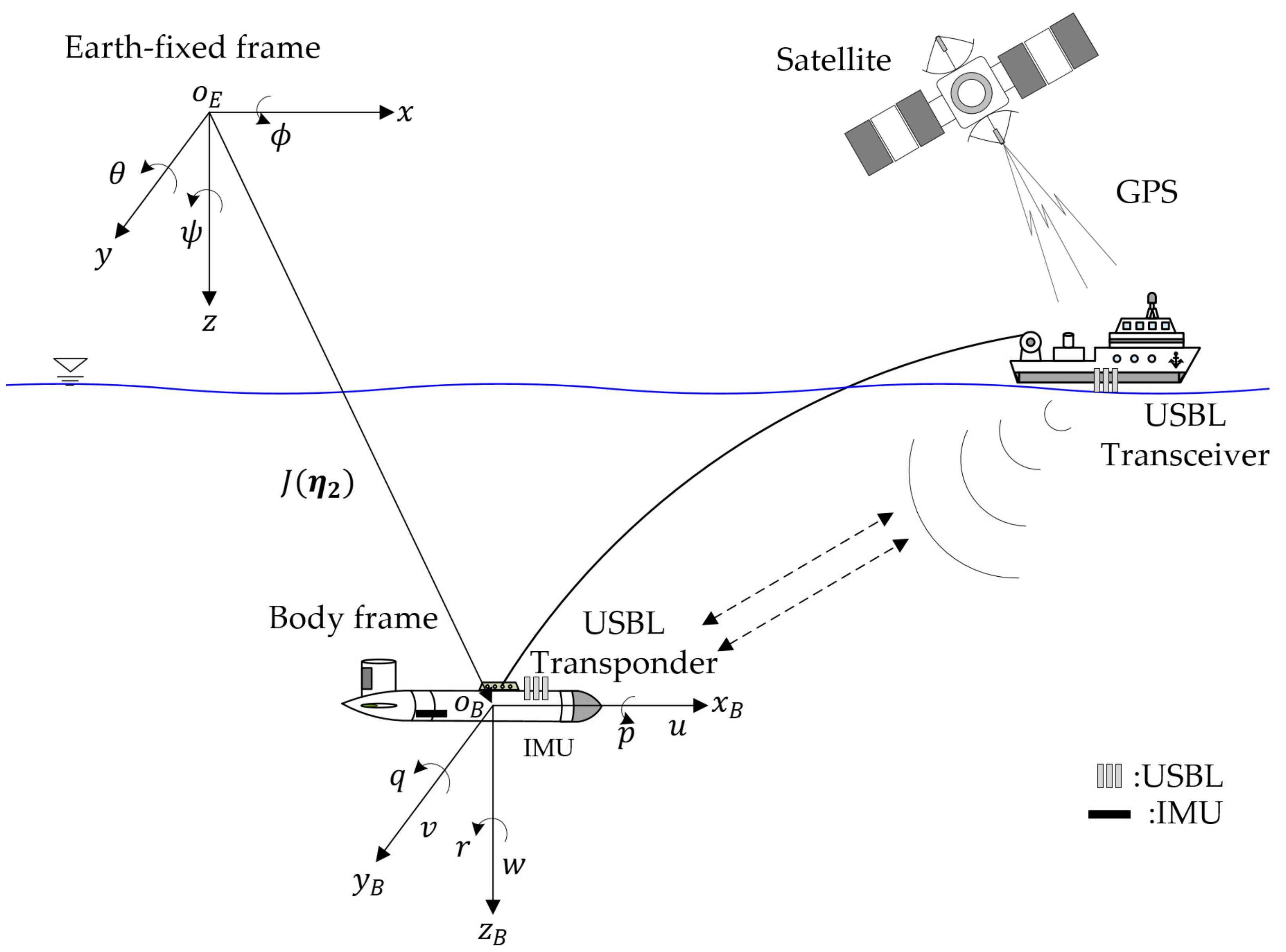
3. Mathematical Model

3.1. Dynamic Towfish Model

Figure 2 shows the forces acting on the towfish. Let ${\mathit{f}}_{\mathit{c}}\in R^3$ be the towed force, ${\mathit{f}}_{\mathit{a}}\in R^3$ be the actuator forces, such as the drag forces generated by the elevator angles ${\delta }_r$ and ${\delta }_l$, and the rudder angle ${\delta }_R$, and ${\mathit{f}}_{\mathit{b}}\in R^6$ be the force generated by the weight and buoyant force. Then, the six degree-of-freedom equations of motion of the towfish can be expressed as follows:

$$M\dot{\mathit{\nu }}+C\left(\mathit{\nu }\right)\mathit{\nu }+D\left(\mathit{\nu }\right)\mathit{\nu }=\left(\begin{array}{c}{\mathit{f}}_{\mathit{c}}\\ {\mathit{r}}_c\times {\mathit{f}}_{\mathit{c}}\end{array}\right)+\left(\begin{array}{c}{\mathit{f}}_{\mathit{a}}\\ {\mathit{r}}_a\times {\mathit{f}}_{\mathit{a}}\end{array}\right)+{\mathit{f}}_{\mathit{b}},$$

(1)

where $\mathit{\nu }={\left(u,v,w,p,q,r\right)}^T\in R^6$, ($u,v,w$) is the linear velocity of the towfish with respect to the body frame, $\left(p,q,r\right)$ is the angular velocity, and ${\mathit{r}}_c, {\mathit{r}}_a\in R^3$ are the position vectors from the center of gravity to the towing point and the center of the actuators, respectively.

Assuming that the shape of the towfish is a symmetrical cylinder, $M$, $C\left(\mathit{\nu }\right)$ and $D\left(\mathit{\nu }\right)$ are given as follows [31,32]:

$$M=M_{RB}+M_A\in R^{6\times 6},$$

(2)

$$M_{RB}=\left(\begin{array}{cccccc}m& 0& 0& 0& m{z}_g& -m{y}_g\\ 0& m& 0& -m{z}_g& 0& m{x}_g\\ 0& 0& m& m{y}_g& -m{x}_g& 0\\ 0& -m{z}_g& m{y}_g& I_{xx}& 0& 0\\ m{z}_g& 0& -m{x}_g& 0& I_{yy}& 0\\ -m{y}_g& m{x}_g& 0& 0& 0& I_{zz}\end{array}\right),$$

(3)

$$M_A=-diag{\left(X_{\dot{u}}, Y_{\dot{v}}, Z_{\dot{w}}, K_{\dot{p}}, M_{\dot{q}}, N_{\dot{r}}\right)}^T,$$

(4)

where $M_{RB}$ and $M_A$ are the rigid-body inertia matrix and hydrodynamic added mass matrix, respectively; $m$ is the mass; ($x_g, y_g, z_g$) is the position of the center of gravity; $I_{xx}$, $I_{yy}$, and $I_{zz}$ are the moments of inertia; and the diagonal components of $M_A$ are the hydrodynamic added mass coefficients.

$$C\left(\mathit{\nu }\right)=C_{RB}\left(\mathit{\nu }\right)+C_A\left(\mathit{\nu }\right)\in R^{6\times 6},$$

(5)

$$\begin{gathered} C_{RB}=\left(\begin{array}{cccc}0& 0& 0& m\left(y_{g}q+z_{g}r\right)\\ 0& 0& 0& -m\left(y_{g}p+w\right)\\ 0& 0& 0& -m\left(z_{g}p-v\right)\\ -m\left(y_{g}q+z_{g}r\right)& m\left(y_{g}p+w\right)& m\left(z_{g}p-v\right)& 0\\ m\left(x_{g}q-w\right)& -m\left(z_{g}r+x_{g}p\right)& m\left(z_{g}q+u\right)& -I_{zz}r\\ m\left(x_{g}r+v\right)& m\left(y_{g}r-u\right)& -m\left(x_{g}p+y_{g}q\right)& I_{yy}q\end{array}\right. \\ \left.\begin{array}{cc}-m\left(x_{g}q-w\right)& -m\left(x_{g}r+v\right)\\ m\left(z_{g}r+x_{g}p\right)& -m\left(y_{g}r-u\right)\\ -m\left(z_{g}q+u\right)& m\left(x_{g}p+y_{g}q\right)\\ I_{zz}r& -I_{yy}q\\ 0& I_{xx}p\\ -I_{xx}p& 0\end{array}\right), \end{gathered}$$

(6)

$$C_A=\left(\begin{array}{cccccc}0& 0& 0& 0& -Z_{\dot{w}}w& Y_{\dot{v}}v\\ 0& 0& 0& Z_{\dot{w}}w& 0& X_{\dot{u}}u\\ 0& 0& 0& -Y_{\dot{v}}v& X_{\dot{u}}u& 0\\ 0& -Z_{\dot{w}}w& Y_{\dot{v}}v& 0& -N_{\dot{r}}r& M_{\dot{q}}q\\ Z_{\dot{w}}w& 0& X_{\dot{u}}u& N_{\dot{r}}r& 0& -K_{\dot{p}}p\\ -Y_{\dot{v}}v& X_{\dot{u}}u& 0& -M_{\dot{q}}q& K_{\dot{p}}p& 0\end{array}\right),$$

(7)

where $C_{RB}\left(\mathit{\nu }\right)$ and $C_A\left(\mathit{\nu }\right)$ are the rigid-body Coriolis and centripetal matrix and the hydrodynamic Coriolis and centripetal matrix, respectively.

Because the towing speed of the target towfish is not high (less than 2$\mathrm{m}/\mathrm{s}$), nonlinear damping with a quadratic form of the towing speed can be neglected. The damping terms can then be simplified as follows [33]:

$$D\left(\mathit{\nu }\right)=D+D_n\left(\mathit{\nu }\right)\approx D\in R^{6\times 6},$$

(8)

$$D=-diag{\left(X_u, Y_v, Z_w, K_p, M_q, N_r\right)}^T,$$

(9)

where $D$ and $D_n\left(\mathit{\nu }\right)$ are the linear damping matrix and nonlinear damping matrix, respectively, and the diagonal components of $D$ are negative scalar coefficients.

Let $\mathit{a}\times \mathit{b}=S\left(\mathit{a}\right)\mathit{b}$, $\mathit{a}=(a_x, a_y, a_z){ }^T$, and $\mathit{b}\in R^3$, where $S\left(\mathit{a}\right)$ is a skew symmetric matrix and is given as follows:

$$S\left(\mathit{a}\right)=\left(\begin{array}{ccc}0& -a_z& a_y\\ a_z& 0& -a_x\\ -a_y& a_x& 0\end{array}\right),$$

(10)

Then, the right side of Equation (1) can be rewritten as

$$\tau =\left(\begin{array}{c}{I}_{3\times 3}\\ \mathit{S}\left({\mathit{r}}_{\mathit{c}}\right)\end{array}\right){\mathit{f}}_{\mathit{c}}+\left(\begin{array}{c}{I}_{3\times 3}\\ \mathit{S}\left({\mathit{r}}_{\mathit{a}}\right)\end{array}\right){\mathit{f}}_{\mathit{a}}+{\mathit{f}}_{\mathit{b}},$$

(11)

$${\mathit{f}}_{\mathit{b}}=\left(\begin{array}{c}-\left(W-B\right)\mathrm{s}\theta \\ \left(W-B\right)s\theta \sin \varphi \\ \left(W-B\right)c\theta \mathrm{c}\varphi \\ (y_{g}W-y_{b}B)\mathrm{c}\theta \mathrm{c}\varphi -\left(z_{g}W-z_{b}B\right)c\theta \mathrm{s}\varphi \\ -\left(z_{g}W-z_{b}B\right)s\theta -\left(x_{g}W-x_{b}B\right)c\theta \mathrm{c}\varphi \\ (x_{g}W-x_{b}B)c\theta \mathrm{s}\varphi +\left(y_{g}W-y_{b}B\right)\mathrm{s}\theta \end{array}\right),$$

(12)

where ($x_b, y_b, z_b$) is the position of the center of buoyancy, and $c$, $s$,$\varphi$, and $\theta$ are the cosine function, sine function, roll angle, and pitch angle, respectively.

Meanwhile, the position of the underwater towfish cannot be obtained directly using the global positioning system (GPS), as shown in Figure 3. Thus, we used the USBL system mounted on the mother ship and towfish for underwater positioning, and the attitude with respect to the body frame is obtained through the IMU. Let $\mathit{\eta }={\left({\mathit{\eta }}_1^T, {\mathit{\eta }}_2^T\right)}^T$, ${\mathit{\eta }}_1={\left(x,y,z\right)}^T$, and ${\mathit{\eta }}_2={\left(\varphi , \theta ,\psi \right)}^T$, where ($x,y,z)$ is the position with respect to the fixed frame, and ($\varphi , \theta ,\psi$) are the roll, pitch, and yaw (heading) angles, respectively. The linear and angular velocities with respect to the fixed frame are given by

$$\dot{\mathit{\eta }}=J\left({\mathit{\eta }}_2\right)\mathit{\nu },$$

(13)

$$J\left({\mathit{\eta }}_2\right)=\left(\begin{array}{cc}{J}_1\left({\mathit{\eta }}_2\right)& 0_{3\times 3}\\ 0_{3\times 3}& J_2\left({\mathit{\eta }}_2\right)\end{array}\right),$$

(14)

$$J_1\left({\mathit{\eta }}_2\right)=\left(\begin{array}{ccc}c\psi \mathrm{c}\theta & -s\psi c\psi +c\psi s\theta \mathrm{s}\varphi & s\psi s\varphi +c\psi c\varphi s\theta \\ s\psi c\theta & c\psi c\varphi +s\varphi s\theta s\psi & -c\psi s\varphi +s\theta s\psi c\varphi \\ -s\theta & c\theta s\varphi & c\theta c\varphi \end{array}\right),$$

(15)

$$J_2\left({\mathit{\eta }}_2\right)=\left(\begin{array}{ccc}1& s\varphi t\theta & c\varphi t\theta \\ 0& c\varphi & -s\varphi \\ 0& s\varphi /c\theta & c\varphi /c\theta \end{array}\right),$$

(16)

where $t$ represents the tangent function.

3.2. Dynamic Model of the Towing Cable

The mathematical model of the towing cable is frequently formulated using the lumped-mass method. The concept of the lumped-mass method is shown in Figure 4a. The towing cable is modeled as ($n-1$) discrete masses interconnected by linear springs that do not have weight, and it is assumed that the drag force, weight, and added mass force acting on the towing cable are concentrated on each mass [34].

As shown in Figure 4a, the forces acting on the $j^{th}$ node (mass) consist of drag forces, tension, and weight. Let $f_{dxj}$, $f_{dyj}$, and $f_{dzj}$ be the drag forces along the $x, y$, and $z$-axes, and $T_j$ and $T_{j-1}$ be the tensions at the $j^{th}$ node and ${\left(j+1\right)}^{th}$ node, respectively. In addition, ${\delta }_j$ is the weight in water, and $l_j$ is the length between the $j^{th}$ node and the ${\left(j+1\right)}^{th}$ node.

In Figure 4b, $xyz$ is the earth-fixed frame, and ${\xi }_{xj}{\xi }_{yj}{\xi }_{zj}$ is the body frame attached to the $j^{th}$ node, where the ${\xi }_{xj}$-axis is defined as the tangential direction of the towing cable, and the ${\xi }_{yj}$ and ${\xi }_{zj}$-axes are defined as the normal directions with respect to the ${\xi }_{xj}$-axis; in addition, the ${\xi }_{xj}{\xi }_{yj}{\xi }_{zj}$ frame is determined by rotating the $xyz$ frame by ${\overline{\alpha }}_j$ around the $z$-axis and ${\overline{\beta }}_j$ around the $y$-axis, ${\alpha }_j$ is the angle between the $x-z$ plane and the cable formed by the $j^{th}$ and ${\left(j+1\right)}^{th}$ nodes, and ${\beta }_j$ is the angle formed by the $x-y$ plane. Therefore, the ${\xi }_{xj}{\xi }_{yj}{\xi }_{zj}$ frame at the $j^{th}$ node can be obtained by

$$\left(\begin{array}{c}{\xi }_{xj}\\ {\xi }_{yj}\\ {\xi }_{zj}\end{array}\right)=\begin{array}{c}\Omega \end{array}\left(\begin{array}{c}x\\ y\\ z\end{array}\right), \begin{array}{c}\Omega \end{array}=\left(\begin{array}{ccc}c{\overline{\alpha }}_{j}c{\overline{\beta }}_j& s{\overline{\alpha }}_{j}c{\overline{\beta }}_j& s{\overline{\beta }}_j\\ -s{\overline{\alpha }}_j& c{\overline{\alpha }}_j& 0\\ -c{\overline{\alpha }}_{j}s{\overline{\beta }}_j& -s{\overline{\alpha }}_{j}s{\overline{\beta }}_j& c{\overline{\beta }}_j\end{array}\right),$$

(17)

The drag forces in the tangential ($f_{dtj}$) and normal ($f_{dnj}$) directions can be expressed as follows:

$$\begin{gathered} f_{dtj}=-\frac{1}{2}\rho C_{Dtj}\pi D_j\frac{l_j+l_{j-1}}{2}\left|u_{tj}\right|u_{tj}, \\ {f}_{dnj}=-\frac{1}{2}\rho C_{Dnj}{D}_j\frac{l_j+l_{j-1}}{2}\left|u_{nj}\right|u_{nj}, \end{gathered}$$

(18)

where $\rho$ is the water density, $D_j$ is the outer diameter of the cable, $C_{Dtj}$ and $C_{Dnj}$ are the drag force coefficients, and $u_{tj}$ are $u_{nj}$ are the tangential and normal speed components, respectively. The drag force components acting on the ${\xi }_{xj}{\xi }_{yj}{\xi }_{zj}$ frame are given by

$$\begin{gathered} f_{d{\xi }_{xj}}=f_{dtj}, \\ {f}_{d{\xi }_{yj}}=f_{dnj}c{\gamma }_j, \\ {f}_{d{\xi }_{zj}}=f_{dnj}s{\gamma }_j. \end{gathered}$$

(19)

In addition, the drag force components acting on the $xyz$ frame are given by

$$\left(\begin{array}{c}{f}_{dxj}\\ f_{dyj}\\ f_{dzj}\end{array}\right)={\Omega }^{-1}\left(\begin{array}{c}{f}_{d{\xi }_{xj}}\\ f_{d{\xi }_{yj}}\\ f_{d{\xi }_{zj}}\end{array}\right),$$

(20)

Next, we determine how to calculate the added mass acting on the $j^{th}$ node. Letting the acceleration components at the $j^{th}$ node be $\ddot{x}$, $\ddot{y}$, and $\ddot{z}$, the corresponding acceleration component on the ${\xi }_{xj}{\xi }_{yj}{\xi }_{zj}$ frame is obtained as follows [35]:

$$\left(\begin{array}{c}{a}_{{\xi }_{xj}}\\ a_{{\xi }_{yj}}\\ a_{{\xi }_{zj}}\end{array}\right)=\begin{array}{c}\Omega \end{array}\left(\begin{array}{c}\ddot{x}\\ \ddot{y}\\ \ddot{z}\end{array}\right),$$

(21)

where the acceleration component in the tangential direction $a_{{\xi }_{xj}}$ is expressed by $a_{tj}$ and the ${\xi }_{yj}$ and ${\xi }_{zj}$ axis acceleration components in normal directions $a_{{\xi }_{yj}}$ and $a_{{\xi }_j}$ are expressed by $a_{nj}c{\gamma }_j$ and $a_{nj}s{\gamma }_j$. Thus, the added mass forces $f_{atj}$, $f_{a{\xi }_{yj}}$, and $f_{a{\xi }_{zj}}$ acting on the $j^{th}$ node are expressed as follows:

$$\begin{gathered} f_{atj}=-\rho \frac{D_j^2\pi }{4}{C}_{atj}\frac{l_j+l_{j-1}}{2}{a}_{tj}=-A_{tj}{a}_{tj}, \\ {f}_{a_{{\xi }_{yj}}}=-\rho \frac{D_j^2\pi }{4}{C}_{anj}\frac{l_j+l_{j-1}}{2}{a}_{{\xi }_{yj}}=-A_{nj}{a}_{{\xi }_{yj}}, \\ {f}_{a_{{\xi }_{zj}}}=-\rho \frac{D_j^2\pi }{4}{C}_{anj}\frac{l_j+l_{j-1}}{2}{a}_{{\xi }_{zj}}=-A_{nj}{a}_{{\xi }_{zj}}, \end{gathered}$$

(22)

where $C_{atj}$ and $C_{anj}$ are the added mass coefficients, and $A_{tj}$ and $A_{nj}$ are the tangential and normal added mass on the $j^{th}$ node, respectively. The components of the added mass force on the $xyz$ frame are then obtained by

$$\left(\begin{array}{c}{f}_{axj}\\ f_{ayj}\\ f_{azj}\end{array}\right)={\begin{array}{c}\Omega \end{array}}^{-1}\left(\begin{array}{c}{f}_{atj}\\ f_{a{\xi }_{yj}}\\ f_{a{\xi }_{zj}}\end{array}\right),$$

(23)

Using Equations (23) and (24), $f_{axj}$ is calculated as follows:

$$\begin{gathered} f_{axj}=-c{\overline{\alpha }}_{j}c{\overline{\beta }}_j{A}_{tj}{a}_{tj}+\mathrm{s}{\overline{\alpha }}_j{A}_{nj}{a}_{{\xi }_{yj}}+\mathrm{c}{\overline{\alpha }}_j\mathrm{s}{\overline{\beta }}_j{A}_{nj}{a}_{{\xi }_{zj}}, \\ =-c{\overline{\alpha }}_{j}c{\overline{\beta }}_j{A}_{tj}\left(c{\overline{\alpha }}_{j}c{\overline{\beta }}_j\ddot{x}+\mathrm{s}{\overline{\alpha }}_j\mathrm{c}{\overline{\beta }}_j\ddot{y}+\mathrm{s}{\overline{\beta }}_j\ddot{z}\right), \\ +\mathrm{s}{\overline{\alpha }}_j{A}_{nj}\left(-s{\overline{\alpha }}_j\ddot{x}+c{\overline{\alpha }}_j\ddot{y}\right)+\mathrm{c}{\overline{\alpha }}_j\mathrm{s}{\overline{\beta }}_j{A}_{nj}\left(-c{\overline{\alpha }}_{j}s\overline{\beta }\ddot{x}-s{\overline{\alpha }}_{j}s\overline{\beta }\ddot{y}+c\overline{\beta }\ddot{z}\right). \end{gathered}$$

(24)

Letting $f_{axj}=X_{xj}\ddot{x}+X_{yj}\ddot{y}+X_{zj}\ddot{z}$, $X_{xj}$, $X_{yj}$, and $X_{zj}$ can be obtained by

$$\begin{gathered} X_{xj}=-c^2{\overline{\alpha }}_j{c}^2{\overline{\beta }}_j{A}_{tj}-\left(1-c^2{\overline{\alpha }}_j{c}^2{\overline{\beta }}_j\right)A_{nj}, \\ {X}_{yj}=\left(A_{nj}-A_{tj}\right)s{\overline{\alpha }}_{j}c{\overline{\alpha }}_j{c}^2{\overline{\beta }}_j, \\ {X}_{zj}=\left(A_{nj}-A_{tj}\right)c{\overline{\alpha }}_{j}s{\overline{\beta }}_{j}c{\overline{\beta }}_j. \end{gathered}$$

(25)

The mathematical model of the towing cable at the $j^{th}$ node can be obtained by calculating the added mass forces along the $y$- and $z$-axes in the same way.

$$\left(\begin{array}{ccc}{m}_{11j}& m_{12j}& m_{13j}\\ m_{21j}& m_{22j}& m_{23j}\\ m_{31j}& m_{32j}& m_{33j}\end{array}\right)\left(\begin{array}{c}\ddot{x}\\ \ddot{y}\\ \ddot{z}\end{array}\right)=\left(\begin{array}{c}{F}_{xj}\\ F_{yj}\\ F_{zj}\end{array}\right),$$

(26)

$$\begin{gathered} m_{11j}=M_j+c^2{\overline{\alpha }}_j{c}^2{\overline{\beta }}_j{A}_{tj}+\left(1-c^2{\overline{\alpha }}_j{c}^2{\overline{\beta }}_j\right)A_{nj}, \\ {m}_{12j}=m_{21j}=\left(A_{tj}-A_{nj}\right)s{\overline{\alpha }}_{j}c{\overline{\alpha }}_j{c}^2{\overline{\beta }}_j, \\ {m}_{13j}=m_{31j}=\left(A_{tj}-A_{nj}\right)c{\overline{\alpha }}_{j}s{\overline{\beta }}_{j}c{\overline{\beta }}_j, \\ {m}_{22j}=M_j+s^2{\overline{\alpha }}_j{c}^2{\overline{\beta }}_j{A}_{tj}+\left(1-s^2{\overline{\alpha }}_j{c}^2{\overline{\beta }}_j\right)A_{nj}, \\ {m}_{23j}=m_{32j}=\left(A_{tj}-A_{nj}\right)s{\overline{\alpha }}_{j}s{\overline{\beta }}_{j}c{\overline{\beta }}_j, \\ {m}_{33j}=M_j+s^2{\overline{\beta }}_j{A}_{tj}+c^2{\overline{\beta }}_j{A}_{nj}, \\ {F}_{xj}=T_{j}c{\overline{\beta }}_{j}c{\overline{\alpha }}_j-T_{j-1}c{\overline{\beta }}_{j-1}c{\overline{\alpha }}_{j-1}+f_{dxj}, \\ {F}_{yj}=T_{j}c{\overline{\beta }}_{j}s{\overline{\alpha }}_j-T_{j-1}c{\overline{\beta }}_{j-1}s{\overline{\alpha }}_{j-1}+f_{dvj}, \\ {F}_{zj}=T_{j}s{\overline{\beta }}_j-T_{j-1}s{\overline{\beta }}_{j-1}+f_{dzj}-{\delta }_j, \end{gathered}$$

(27)

Here, the cable tension $T_j$ can be obtained by

$$T_j=E_j{A}_j\left(\frac{l_j}{\overline{l_j}}-1\right),$$

(28)

where $E_j$ is the Young’s modulus of the towing cable, $A_j$ is the cross-sectional area, and $\overline{l_j}$ is the length without deformation.

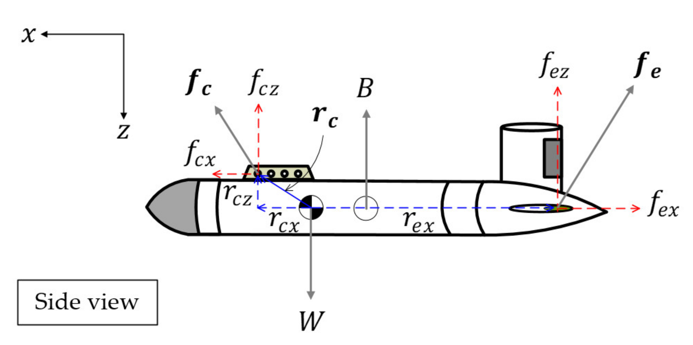
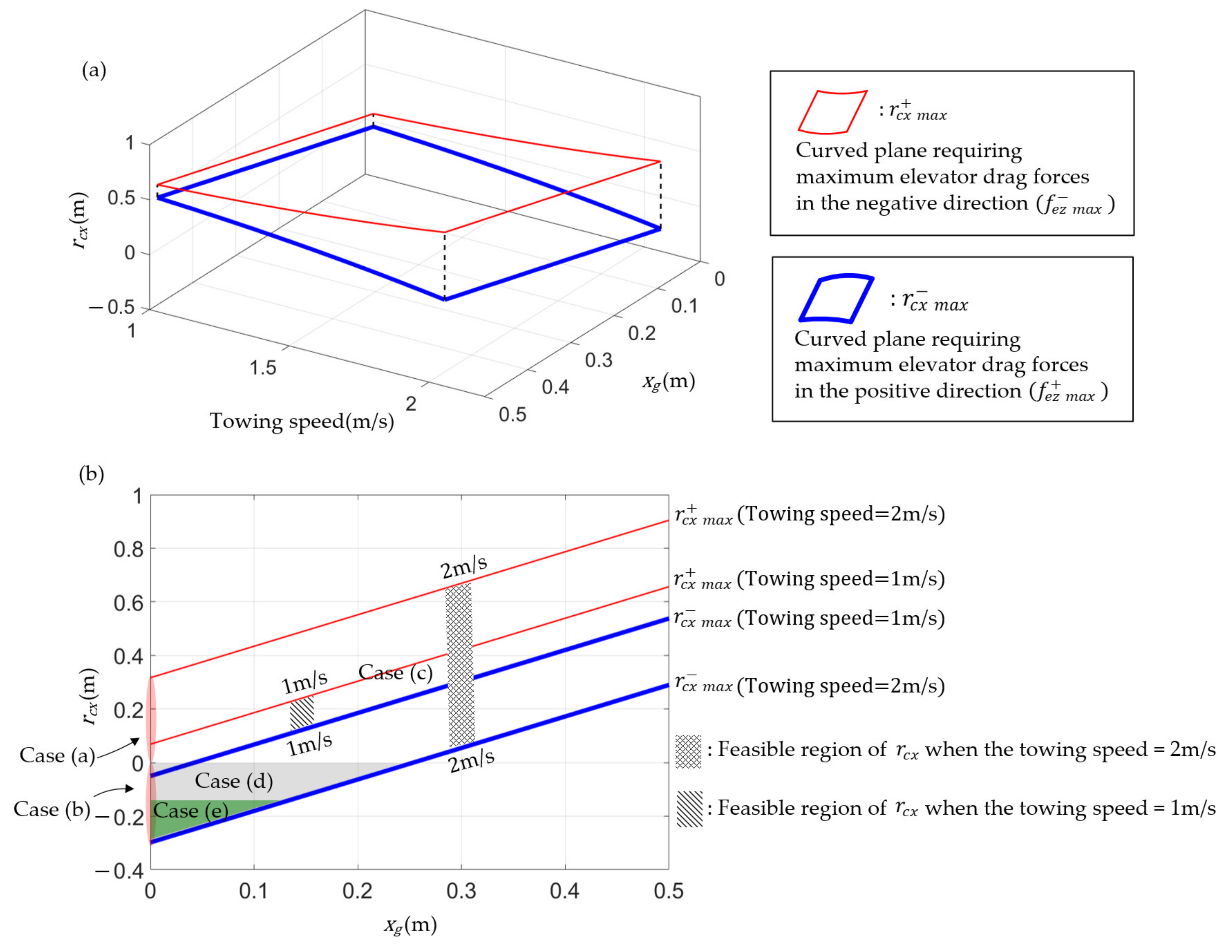
4. Feasible Region of the Towing Point for Attitude Control

The roll motion is stabilized automatically by the weight and vertical towing force; thus, we discuss the pitch and yaw control in connection with the positions of the towing point, the center of gravity, and the towing speed.

4.1. Feasible Towing Point for Pitch Control

Figure 5 shows the forces acting on the towfish in the $x-z$ plane. Here, ${\mathit{f}}_{\mathit{c}}={\left(f_{cx}, f_{cz}\right)}^T$ is the towing force, ${\mathit{f}}_{\mathit{e}}={\left(f_{ex}, f_{ez}\right)}^T$ is the drag force generated by the elevators, and ${\mathit{r}}_{\mathit{c}}={\left(r_{cx}, r_{cz}\right)}^T$ and ${\mathit{r}}_{\mathit{e}}={\left(r_{ex},0\right)}^T$ are the position vectors from the center of gravity to the towing position and from the center of gravity to the center of the elevators, respectively. The pitching moment generated by these forces can be expressed as follows:

$$M_y={\mathit{r}}_{\mathit{c}}\otimes {\mathit{f}}_{\mathit{c}}+{\mathit{r}}_{\mathit{e}}\otimes {\mathit{f}}_{\mathit{e}}+f_{b5},$$

(29)

here, $f_{b5}$ is the fifth component in Equation (12), and $\otimes$ is the outer product in the plane and is calculated as follows:

$$\begin{gathered} \mathit{a}\otimes \mathit{b}={\left(E\mathit{a}\right)}^T\mathit{b}=\left(E^T{\mathit{a}}^T\right)\mathit{b}, \mathit{a},\mathit{b}\in R^2, \\ E=\left(\begin{array}{cc}0& -1\\ 1& 0\end{array}\right), \end{gathered}$$

(30)

where $E$ is the rotation matrix that rotates ${90}^{°}$ counterclockwise on a plane.

When controlling the attitude of the towfish, it is difficult to secure the stability of the towfish if the center of gravity is behind the center of buoyancy. Thus, as shown in Figure 6, five cases (cases (a)–(e)) in which the position of the center of gravity is the same as that at or before the center of buoyancy are selected and discussed. In the following, it is assumed that the center of buoyancy is located at the center of the body of the towfish.

4.1.1. When the Center of Gravity Is the Same as the Center of Buoyancy (Cases (a) and (b))

In cases (a) and (b), the center of gravity is located at the center of the buoyancy. As a difference between these two cases, the towing point is located before and behind the center of gravity. Here, the effect of the restoring force term $f_{b5}$ in Equation (12) can be ignored because $z_g=z_b=x_g=x_b=0$. Therefore, $r_{cx}$ in equilibrium with the maximum elevator forces in the positive and negative directions in Equation (29) can be obtained as follows:

$$\begin{gathered} r_{cx max}^{+}=\frac{r_{cz}{f}_{cx}+r_{ex}{f}_{ez max}^{-}}{f_{cz}}, \\ {r}_{cx max}^{-}=-\left(\frac{-r_{cz}{f}_{cx}+r_{ex}{f}_{ez max}^{+}}{f_{cz}}\right), \end{gathered}$$

(31)

where $f_{ez max}^{+}$ and $f_{ez max}^{-}$ are defined as the maximum drag forces of elevators in the positive and negative directions, respectively, and $r_{cx max}^{+}$ and $r_{cx max}^{-}$ are defined as the maximum towing points where the pitching moment occurs in the positive and negative directions, respectively. In addition, if the towing point is located outside of $r_{cx max}^{+}$ and $r_{cx max}^{-}$, the pitch motion cannot be controlled by the drag forces of the given elevators.

4.1.2. When the Center of Gravity Is Before the Center of Buoyancy (Cases (c)–(e))

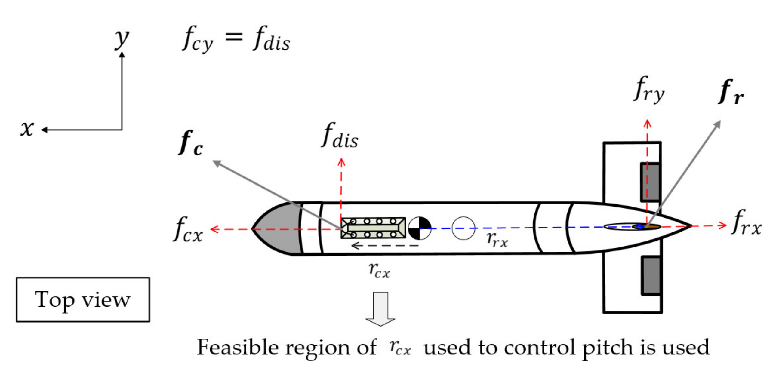
Cases (c)–(e) are classified according to the position of the towing point. Case (c) is the case in which the towing point is before the center of gravity, Case (d) is between the center of gravity and the center of buoyancy, and Case (e) is behind the center of buoyancy. Because the center of gravity and the center of buoyancy are at different positions, the restoring force must be considered. Assuming that the changes in the pitch and roll motions are extremely small, that is, $\theta \approx 0^{°}$ and $\varphi \approx 0^{°}$, $f_{b5}=-\left(z_{g}W-z_{b}B\right)s\theta -\left(x_{g}W-x_{b}B\right)c\theta \mathrm{c}\varphi$ in Equation (12) can be simplified to $-x_{g}W$. Hence, the towing points in equilibrium with the maximum elevator forces in the positive and negative directions can be obtained as follows:

$$\begin{gathered} r_{cx max}^{+}=\frac{r_{cz}{f}_{cx}+r_{ex}{f}_{ez max}^{-}+x_{g}W}{f_{cz}}, \\ {r}_{cx max}^{-}=-\left(\frac{-r_{cz}{f}_{cx}+r_{ex}{f}_{ez max}^{+}+x_{g}W}{f_{cz}}\right), \end{gathered}$$

(32)

To find the feasible region of the towing point, numerical simulations were conducted using Equations (31) and (32). In addition, $f_{cx}$, $f_{ez max}^{-}$, and $f_{ez max}^{+}$ were determined according to the towing speed, and other components except $f_{cz}$ are given by the specifications of the towfish (as illustrated in Table 1). Moreover, $f_{cz}$ was set to be equal to the underwater weight of the towfish, and these two forces are assumed to be in static equilibrium. The underwater weight $\left(W-B\right)$ is $2450 \mathrm{N}$, $r_{cz}=0.2 \mathrm{m}$, and $r_{ex}=1.7 \mathrm{m}$ if $x_g$ is at the center of body. In addition, the drag forces of the elevators were calculated using Equation (35) given in Section 5.

Figure 7a shows the feasible region of the towing point when the towing speed changes from $1$ to $2 \mathrm{m}/\mathrm{s}$ and $x_g$ changes from $0$ to $0.5 \mathrm{m}$. The curved plane determined by the red lines ($r_{cx max}^{+}$) contains the maximum value of $r_{cx}$ generating a moment in the positive direction, and the curved plane $r_{cx max}^{-}$ contains the maximum value of $r_{cx}$ generating a moment in the negative direction. On the two curved planes, the elevators are required to exert maximum drag forces $f_{ez max}^{-}$ and $f_{ez max}^{+}$ for pitch control; this implies that pitch control is difficult to accomplish if $r_{cx}$ lies on the two curved planes. Therefore, we need to choose the value of $r_{cx}$ (the position of the towing point) in the area between the two curved planes to control the pitch motion more easily.

Figure 7b shows the feasible regions obtained for the five cases shown in Figure 6. The feasible region for Case (c) is wider than that of other cases; in addition, cases (d) and (e) have narrow feasible regions, which means that the pitch control is difficult to achieve owing to the narrow range of $f_{ez max}^{+}$. Meanwhile, cases (a) and (b) are special cases in which $x_g=0$ and the range of the towing point for the pitch control is similarly assigned in the positive and negative directions. In addition, for all cases, the feasible region of the towing point widens as the towing speed increases because the drag force generated by the elevator is proportional to the square of the towing speed.

4.2. Yaw Control

The pitching moment is closely related to the positions of the center of gravity, center of buoyancy, and towing point; however, the yawing moment does not occur if there is no initial error or disturbance. In what follows, we investigate the range of the disturbance in which the yaw control can be achieved using the drag force of the rudder. Note that this discussion is based on the feasible region of the towing point described in Section 4.1.

Figure 8 shows the forces acting on the towfish in the $x-y$ plane (horizontal plane). Let $f_{cx}$ and $f_{cy}$ be the towing forces in the longitudinal and lateral directions, respectively, and $f_{cy}$ be regarded as a disturbance ($f_{dis}$), that is, $f_{cy}=f_{dis}$. The yawing moment can then be given by

$$M_z=r_{cx}{f}_{dis}+r_{rx}{f}_{ry}+f_{b6},$$

(33)

where $r_{rx}$ is a vector from the center of gravity to the center of the rudder, and $f_{b6}$ is the sixth component of ${\mathit{f}}_{\mathit{b}}$ in Equation (12). Assuming that the changes in the pitch and roll motions are extremely small, that is, $\theta \approx 0^{°}$, $\varphi \approx 0^{°}$, $f_{b6}=(x_{g}W-x_{b}B)c\theta \mathrm{s}\varphi +\left(y_{g}W-y_{b}B\right)\mathrm{s}\theta$ can be simplified to zero. Therefore, $f_{dis}$ in equilibrium with the maximum rudder force in the positive and negative directions can be obtained as follows:

$$\begin{gathered} f_{dis max}^{+}=\frac{r_{rx}{f}_{ry max}^{-}}{r_{cx max}^{+}}, \\ {f}_{dis max}^{-}=-\left(\frac{-r_{rx}{f}_{ry max}^{+}}{r_{cx max}^{-}}\right), \end{gathered}$$

(34)

where $f_{ry max}^{+}$ and $f_{ry max}^{-}$ are defined as the maximum drag forces of the rudder in the positive and negative directions, respectively, and $f_{dis max}^{+}$ and $f_{dis max}^{-}$ are the maximum disturbances in the positive and negative directions, which can be handled by the rudder.

Numerical simulations were conducted using Equation (34) to determine the allowable range of the magnitude of the disturbance. In addition, $f_{ry max}^{-}$ and $f_{ry max}^{+}$ are determined according to the towing speed, $r_{rx}$ is determined by the specifications of the towfish, and $r_{cx max}^{+}$ and $r_{cx max}^{-}$ are the values obtained in Section 4.1. If $x_g$ is at the center of the body, $r_{rx}=1.7 \mathrm{m}$.

Figure 9 shows the allowable range of the disturbance when $x_g=0.3 \mathrm{m}$ and the towing speed and towing point change. For reference, the allowable ranges for different values of $x_g$ are shown in Figure 10. As shown by the thick red and blue lines, the maximum drag forces of the rudder in the positive and negative directions are required for yaw control; thus, the lines indicate whether the yaw control can be conducted sufficiently. From this figure, we know that yaw control can be accomplished in the area marked with a black solid line. Similar to the pitch motion, the rudder can respond to larger disturbances as the towing speed increases.

Figure 10 shows the allowable range of the disturbance where the rudder can perform yaw control according to the changes in towing speed and towing point for each center of gravity position. The allowable range of the disturbance decreases as the position of the center of gravity moves forward; this is because if the center of gravity moves forward, the value of $r_{cx}$ increases, as shown in Figure 7. Thus, a smaller value of $r_{cx}$ is better for yaw control when the same magnitude of disturbance is applied. In addition, as shown in Figure 10a, when the center of gravity is $0 \mathrm{m}$, there are cases in which the allowable range includes negative values of $r_{cx}$.

5. Simulation

5.1. Simulation Conditions

For the simulations, the drag forces generated by the elevators and rudder are obtained as follows:

$$\begin{gathered} f_{ax}=C_H{C}_D+C_H{C}_D+C_V{C}_D, \\ {f}_{ay}=C_V{C}_L, \\ {f}_{az}=C_H{C}_L+C_H{C}_L, \\ {C}_L,C_D=function of \alpha , C_H=0.5\rho s_H{u}^2, C_V=0.5\rho s_V{u}^2, \end{gathered}$$

(35)

where $f_{ax}$, $f_{ay}$, and $f_{az}$ are the forces exerted by the actuators (elevators and rudder) acting on the $x$, $y$, and $z$-axes, respectively; $s_H$ and $s_V$ are the areas of a single elevator and rudder; and $\rho$, $u$, and $\alpha$ are the density of the water, towing speed, and angle of attack, respectively. In addition, $C_D$ and $C_L$ are the drag and lift coefficients, respectively. The National Advisory Committee for Aeronautics (NACA) provides values of $C_D$ and $C_L$ according to the shape of the airfoil. Because the angle of attack is the same as the angle of the actuator [36], $f_{ax}$, $f_{ay}$, and $f_{az}$ are expressed as functions of the actuator angles. Letting ${\delta }_r$ and ${\delta }_l$ be the angles of the left and right elevators, and ${\delta }_R$ be the rudder angle, from Equations (1) and (11), the mathematical model of the towfish can be expressed as

$$\begin{gathered} M\dot{\mathit{\nu }}+C\left(\mathit{\nu }\right)\mathit{\nu }+D\left(\mathit{\nu }\right)\mathit{\nu }-{\mathit{f}}_{\mathit{b}}-\left(\begin{array}{c}{I}_{3\times 3}\\ \mathit{S}\left({\mathit{r}}_{\mathit{c}}\right)\end{array}\right){\mathit{f}}_{\mathit{c}} \\ =\left(\begin{array}{ccc}-0.065C_H& -0.065C_H& -0.065C_V\\ 0& 0& 0.11C_V\\ 0.11C_H& 0.11C_H& 0\\ 0& 0& 0\\ 0.11C_H{r}_{ex}& 0.11C_H{r}_{ex}& 0\\ 0& 0& 0.11C_V{r}_{rx}\end{array}\right)\left(\begin{array}{c}{\delta }_r\\ {\delta }_l\\ {\delta }_R\end{array}\right), \end{gathered}$$

(36)

where $0.065$ and $0.11$ are the slope of the drag and lift coefficients according to changes in the elevator and rudder angles, respectively, and can be linearized by referring to the values for the NACA 0018 model.

In addition, the attitude controller used for this study is given by

$$\begin{gathered} {\delta }_r,{\delta }_l=K_p\_P\left({\theta }_{ref}-\theta \right)-K_d\_Pq+K_i\_P{{\displaystyle \int }}_0^t\left({\theta }_{ref}-\theta \right), \\ {\delta }_R=K_p\_Y\left({\psi }_{ref}-\psi \right)-K_d\_Yr+K_i\_Y{{\displaystyle \int }}_0^t\left({\psi }_{ref}-\psi \right), \end{gathered}$$

(37)

where $K_p\_P$, $K_d\_P$, and $K_i\_P$ are the control gains of a proportional-integral-derivative (PID) controller used for pitch control, and ${\theta }_{ref}$ and $\theta$ are the target pitch angle (reference value) and current pitch angle, respectively. In addition, $K_p\_Y$, $K_d\_Y$, and $K_i\_Y$ are the control gains of the PID controller used for yaw control, and ${\psi }_{ref}$ and $\psi$ are the reference and current yaw angles, respectively.

Table 2. Parameter values of towfish used for the simulation.

Parameter	Values	Parameter	Values
$m$	$300 \mathrm{kg}$	$M_{\dot{q}}$	$-144.4516 \mathrm{kg}$
$I_{xx}$	$6 {\mathrm{kgm}}^2$	$N_{\dot{r}}$	$-144.4516 \mathrm{kg}$
$I_{yy}$	$309.25{ \mathrm{kgm}}^2$	$X_u$	$-20 \mathrm{kg}/\mathrm{s}$
$I_{zz}$	$309.25{ \mathrm{kgm}}^2$	$Y_v$	$-200 \mathrm{kg}/\mathrm{s}$
$X_{\dot{u}}$	$-12.837 \mathrm{kg}$	$Z_w$	$-200 \mathrm{kg}/\mathrm{s}$
$Y_{\dot{v}}$	$-276.2693 \mathrm{kg}$	$K_p$	$-30{ \mathrm{kgm}}^2/\mathrm{s}$
$Z_{\dot{w}}$	$-276.2693 \mathrm{kg}$	$M_q$	$-300{ \mathrm{kgm}}^2/\mathrm{s}$
$K_{\dot{p}}$	$0 \mathrm{kg}$	$N_r$	$-300{ \mathrm{kgm}}^2/\mathrm{s}$

lists the parameter values used in the simulations. The moments of inertia $I_{xx}$, $I_{yy}$, and $I_{zz}$ were calculated from cylindrical features; $X_{\dot{u}}$, $Y_{\dot{v}}$, $Z_{\dot{w}}$, $K_{\dot{p}}$, $M_{\dot{q}}$, and $N_{\dot{r}}$ were obtained using the specifications of the towfish, and the remaining parameters $X_u$, $Y_v$, $Z_w$, $K_p$, $M_q$, and $N_r$ were selected through simulations.

Table 3. Parameter values of towing cable used for simulation.

Parameter	Values	Parameter	Values
$D$	$22.5 \mathrm{mm}$	$C_{an}$	$1.0$
$W$	$8.9 \mathrm{kN}/\mathrm{km}$	$C_{at}$	$0$
$\delta$	$5 \mathrm{kN}/\mathrm{km}$	$C_{Dn}$	$2.5$
$E$	$3300 \mathrm{kg}/{\mathrm{mm}}^2$	$C_{Dt}$	$0.01$
$L$	$200 \mathrm{m}$	$\overline{l}$	$20 \mathrm{m}$

lists the parameter values of the towing cables. The shape of the cable can be considered as a circular cylinder, and the normal and tangential added mass coefficients $C_{an}$ and $C_{at}$ are set to 1 and zero, respectively. The tangential drag force coefficient $C_{Dt}$ is assumed to be extremely small and set as 0.01, and the normal drag force coefficient $C_{Dn}$ was determined to be 2.5 through simulations. The length of the cable $L$ was selected as $200 \mathrm{m}$ and the length between each node $\overline{l}$ without tension was set to $20 \mathrm{m}$.

The control gains for pitch control $K_p\_P$, $K_d\_P$, and $K_i\_P$ are chosen as 3, 5, and 0.01, respectively, and the gains for yaw control $K_p\_Y$, $K_d\_Y$, and $K_i\_Y$ are 4, 5, and 0.01, respectively. In addition, the angles in the positive and negative directions of the elevators and rudder were limited to 30°.

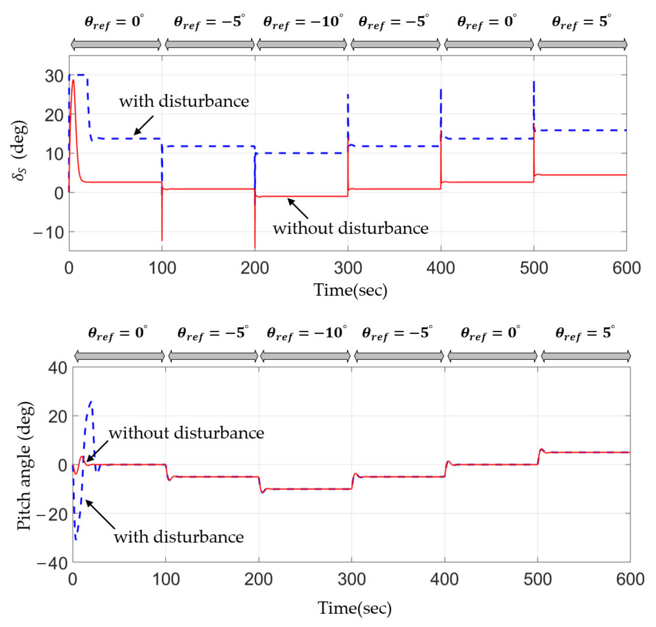
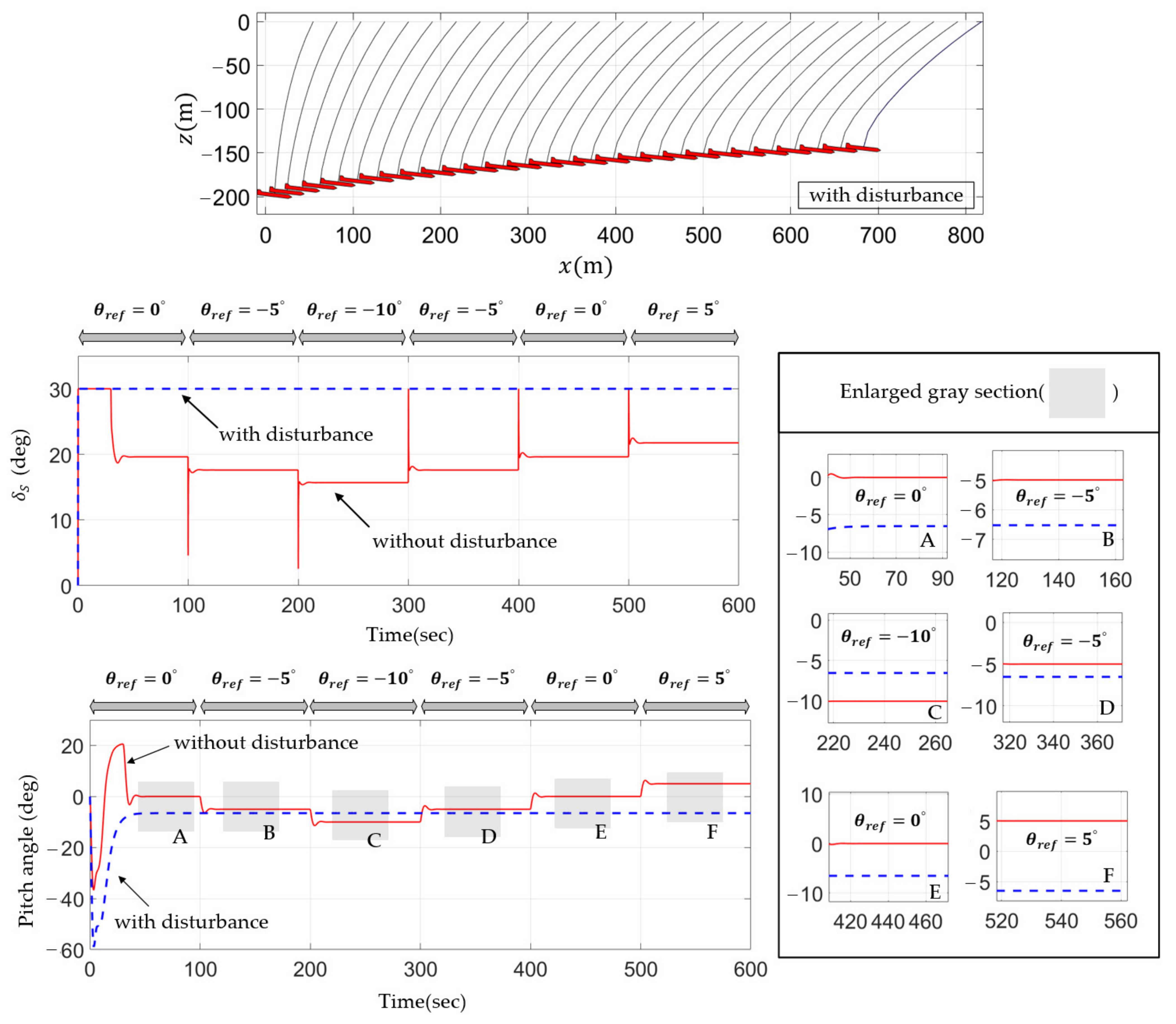
5.2. Pitch Control for Cases (c) and (e)

Table 4. Values of $r_{cx max}^{+}$ and $r_{cx max}^{-}$ according to $x_g$ when the towing speed is $1.5 \mathrm{m}/\mathrm{s}$ and selected $r_{cx}$ for simulation.

$\mathbf{Towing}\mathbf{Speed}=1.5 m/s$	Case (c)	Case (e)
$x_g$	$0.3 \mathrm{m}$	$0.05 \mathrm{m}$
$r_{cx max}^{+}$	$0.5 \mathrm{m}$	$-0.05 \mathrm{m}$
$r_{cx max}^{-}$	$0.2 \mathrm{m}$	$-0.08 \mathrm{m}$
selected $r_{cx}$ for simulation	$0.35 \mathrm{m}$	$-0.06 \mathrm{m}$

shows the maximum values of the towing point generating pitching moment in the positive and negative directions when the center of gravity changes and the towing speed is $1.5 \mathrm{m}/\mathrm{s}$. For the simulation, $r_{cx}$ was selected as $0.35 \mathrm{m}$ in Case (c) and $-0.06 \mathrm{m}$ in Case (e).

Figure 11 shows the simulation results for Cases (c) and (e). The actual size of the towfish is $3.5 \mathrm{m}$ in length and $0.4 \mathrm{m}$ in height, although the length and height were enlarged by approximately 10-fold in the figure to make it easier to understand the motion of the towfish. The synchronous elevator angle ${\delta }_S$ is given by ${\delta }_s=\left({\delta }_r+{\delta }_l\right)/2$. The reference value ${\theta }_{ref}$ was changed to 0°, −5°, −10°, −5°, 0°, and 5° in order, and the current pitch angle tracks the reference value well; however, Case (e) has a narrow region of the towing point, as shown in Figure 7a, and a large elevator angle is required to perform the pitch control. Hence, if a disturbance is applied, it is difficult to achieve the pitch. By contrast, in Case (c), we can also observe that pitch control can be achieved with small elevator angles. Moreover, there is a large spare range of the elevator angles, which means that we can control the pitch motion sufficiently if a disturbance occurs.

In addition, note that the pitch angle of the towfish changed significantly at the beginning part of the simulation because the towing cable is in a transition stage and the towing force is thus unstable at that time.

5.3. Pitch Control for Cases (c) and (e) When Disturbance Is Applied

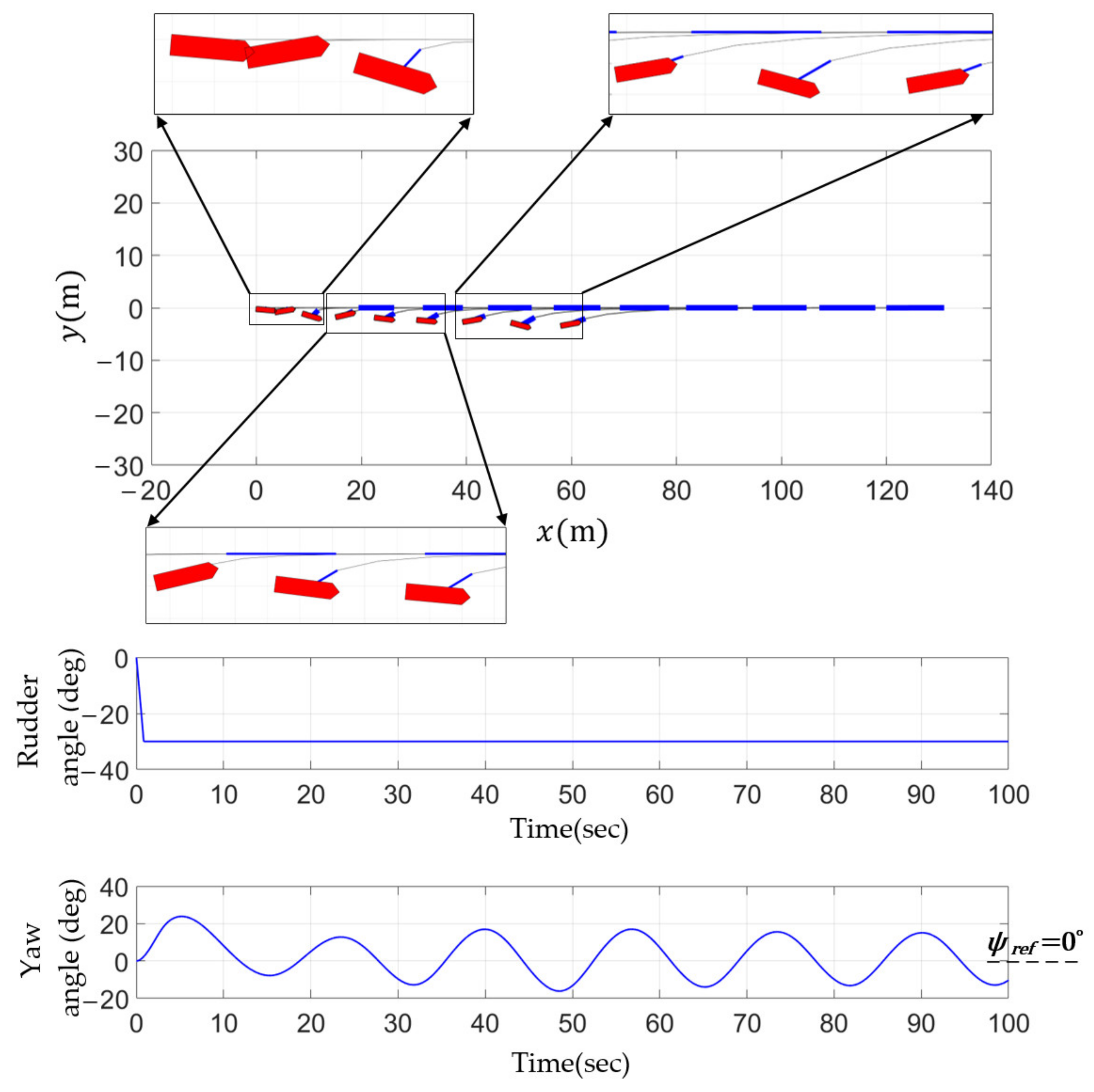
Case (c) has a spare range and is able to respond to additional disturbances, and Case (e) was considered to have difficulty responding to additional disturbances because there was little spare range of the elevator angles. Therefore, in Section 5.3, it is shown that the elevators can handle disturbances in both cases (c) and (e). The simulation was carried out under the same conditions as in Table 4, and a pitching moment of $-200 \mathrm{Nm}$ was continuously applied for cases (c) and (e) as a disturbance.

Figure 12 shows the simulation results when a disturbance of $-200 \mathrm{Nm}$ is applied in Case (c). The animation for this case is analogous to that in Figure 11 and is therefore omitted. The pitch angle can track the reference value ${\theta }_{ref}$ accurately if a disturbance is applied.

Figure 13 shows the simulation results when a disturbance of $-200 \mathrm{Nm}$ is applied in Case (e). Without a disturbance, elevator angles of approximately 20° and 16° are required to track the reference values of ${\theta }_{ref}=$ 0° and 10° (see the red line). Therefore, a spare range of approximately 10° can respond to a disturbance because the maximum elevator angle is 30°; however, if the applied disturbance exceeds the ability of the elevators, the pitch angle cannot be controlled properly (see dotted blue line).

From the results, we know that Case (c) is more advantageous for pitch control than Case (e) because there is enough spare range of elevator angles that can respond to unexpected disturbance.

5.4. Yaw Control

Figure 14 shows the allowable range of disturbance where the yaw control can be achieved under the same conditions as Case (c) in Table 4. The simulation was conducted by selecting points marked with a circle and triangle in the controllable and uncontrollable areas, respectively.

5.4.1. At the Point Marked with a Circle

In this case, the rudder can sufficiently respond to disturbances because the point is located inside the controllable area. First, to emphasize the importance of yaw control, the towfish was towed without controlling the yaw. It is assumed that a yawing moment of $200 \mathrm{Nm}$ is applied continuously as a disturbance. Figure 15 shows the simulation results. For clearer understanding, the $20 \mathrm{m}$ length of cable from the mother ship and the $20 \mathrm{m}$ length of cable from the towfish are drawn by thick blue lines. If the yaw control is not applied (rudder angle = 0°), the yaw angle of the towfish varies in the form of a sine wave, and this motion can distort the image of the sonar, for example, InSAS attached to the towfish. Thus, yaw control is necessary to improve the quality of sonar images.

Figure 16 shows the simulation results when the yaw control is performed. The reference value ${\psi }_{ref}$ was set to 0°. We can confirm that the yaw angle was controlled to 0°; however, the towfish moved while maintaining an offset in the $y$-axis direction owing to the disturbance. To address this problem, the yaw controller in Equation (37) is slightly modified as follows such that it can control the sway (the motion along the $y$-axis) and the yaw angle.

$${\delta }_R=K_p\_Y\left({\psi }_{ref}-\psi \right)-K_d\_Yr+K_i\_Y{{\displaystyle \int }}_0^t\left({\psi }_{ref}-\psi \right)+K_P\_S\left(y_{ref}-y\right),$$

(38)

where $y_{ref}$ and $y$ are the target and current $y$-axis positions, respectively, and $K_P\_S$ is the control gain for sway control. The control gains $K_p\_Y$, $K_d\_Y$, $K_i\_Y$, and $K_p\_S$ are chosen as 10, 5, 0.015, and 3, respectively. Figure 16 also shows the simulation results when yaw and sway control were performed. The towfish can move without an offset error in the $y$-axis position.

5.4.2. At the Point Marked with a Triangle

Figure 17 shows the simulation results at the point marked with a triangle with a disturbance of $350 \mathrm{Nm}$. The controller in Equation (37) was used for yaw control. The triangle is located in an uncontrollable area, and the yaw angle cannot be controlled even if the maximum angle is −30°.

6. Conclusions

This paper discussed an attitude control method for a towfish with two elevators and a single rudder to improve the quality of the image of a sonar system attached to the towfish. A feasible region of the towing point for pitch control in accordance with the variations in the center of gravity and towing speed was presented, and the allowable range of disturbance for yaw control was investigated. Through simulations with the dynamics of the towfish and towing cable, it was demonstrated that the feasible region of the towing point obtained and the allowable range of the disturbance were both correctly selected, and there was a region/range where the attitude control can be applied with relative ease. The results can be summarized as follows.

(1)

When the feasible towing point is located before the center of gravity, attitude control can be achieved even if disturbance is applied;

(2)

When the feasible towing point is located behind the center of gravity, attitude control is difficult to be accomplished sufficiently because there is small spare range of the elevator angles;

(3)

The yaw control is required. Otherwise, the towfish can move in the form of a sine wave if disturbance is applied consistently;

(4)

To track a given path accurately, sway control is required together with the yaw control.

Especially, the results (1) and (2) can be used as an index to determine the position of the towing point and the capacity of the actuators (elevators and rudder) for attitude control at the design stage and in the field. In addition, the results of this study will be applied to the towfish under development and therefore our future work involves performing experiments in the sea using the towfish.

References

1. Pang, S.; Li, Y.; Yi, H. Joint Formation Control with Obstacle Avoidance of Towfish and Multiple Autonomous Underwater Vehicles Based on Graph Theory and the Null-Space-Based Method. Sensors 2019, 19, 2591. [Google Scholar] [CrossRef] [PubMed] [Green Version]
2. Murashima, T.; Aoki, T.; Tsukioka, S.; Hyakudome, S.; Yoshida, H.; Nakajoh, S.; Ishibashi, S.; Sasamoto, R. Thin cable systems for ROV and AUV in JAMSTEC. Oceans 2003, 5, 2695–2700. [Google Scholar]
3. Kostenso, V.; Tolstonogov, A.; Mokeeva, I. The Combined AUV Motion Control with Towed Magnetometer. In Proceedings of the 2019 IEEE Conference on Underwater Technology, Kaohsiung, Taiwan, 16–19 April 2019. [Google Scholar]
4. Wakita, N.; Hiyoshi, H.; Lchikawa, T.; Yamauchi, Y. Development of Autonomous Underwater Vehicle (AUV) for Exploring Deep Sea Marine Mineral Resources. Mitsubishi Heavy Ind. Tech. Rev. 2010, 47, 73–80. [Google Scholar]
5. Yan, Z.; Wu, Y.; Zhang, G. A Real-Time Path Planning Algorithm for AUV in Unknown Underwater Environment Based on Combining PSO and Waypoint Guidance. Sensors 2018, 19, 20. [Google Scholar] [CrossRef] [PubMed] [Green Version]
6. Cao, X.; Sun, H.; Jan, G. Multi-AUV cooperative target search and tracking in unknown underwater environment. Ocean Eng. 2018, 150, 1–11. [Google Scholar] [CrossRef]
7. Park, J.; Kim, N. Dynamics modeling of a semi-submersible autonomous underwater vehicle with a towfish towed by cable. Nav. Archit. Ocean Eng. 2015, 7, 409–425. [Google Scholar] [CrossRef] [Green Version]
8. Go, G.; Ahn, H. Hydrodynamic derivative determination based on CFD and motion simulation for a tow-fish. Appl. Ocean Res. 2019, 82, 191–209. [Google Scholar] [CrossRef]
9. Buckham, B.; Nahon, M.; Seto, M.; Zhao, X.; Lambert, C. Dynamics and control of a towed underwater vehicle system, part 1: Model development. Ocean Eng. 2003, 30, 453–470. [Google Scholar] [CrossRef]
10. Lee, J.; Oh, Y.; Park, S.; Kim, H. Development of towed synthetic aperture sonar system. Korea Soc. Nav. Sci. Technol. 2019, 2, 28–31. [Google Scholar] [CrossRef]
11. Conrad, R.A. Development and Characterization of a Side Scan Sonar Towfish Stabilization Device. Master’s Thesis, University of New Hampshire, Durham, UK, 2006. [Google Scholar]
12. Pilbrow, E.; Hayes, P.; Gough, P. Inertial Navigation System for a Synthetic Aperture Sonar Towfish. In Proceedings of the Electronics New Zealand Conference, Christchurch, New Zealand, 26–28 November 2002. [Google Scholar]
13. Crawford, A. Methods of Determining Towfish Location for Improvement of Side Scan Sonar Image Positioning; Defense Research Reports. Report Number: DRDC-ATLANTIC-TM-2003-019-Technical Memorandum; Defence Research Establishment Atlantic: Dartmouth, NS, Canada, 2002. [Google Scholar]
14. Muscat, M.; Cammarata, A.; Maddio, P.; Sinatra, R. Design and development of a towfish to monitor marine pollution. Euro-Mediterr. J. Environ. Integr. 2018, 3, 1–12. [Google Scholar] [CrossRef]
15. Antonelli, G.; Chiaverini, S.; Finotello, R.; Schiavon, R. Real-time path planning and obstacle avoidance for RAIS: An autonomous underwater vehicle. Ocean Eng. 2001, 26, 216–227. [Google Scholar] [CrossRef]
16. Korte, H. Track Control of a Towed Underwater Sensor Carrier. IFAC Proc. Vol. 2000, 33, 89–94. [Google Scholar] [CrossRef]
17. Pilbrow, E.; Hayes, M. Acoustic Timing Simulation of Active Beacons for Measuring the Tow-Path of a Synthetic Aperture Sonar; Acoustic Research Groups: Christchurch, New Zealand, 2004. [Google Scholar]
18. Fortune, S.; Gough, P.; Hayes, M. A Statistical Method for Autofocus of Synthetic Aperture Sonar Images. In Proceedings of the IVCN 2000, Hamilton, New Zealand, 6 January 2000. [Google Scholar]
19. Cammarata, A.; Sinatra, R. Parameter Study for the Steady-State Equilibrium of a Towfish. Intell. Robot. Syst. 2016, 81, 231–240. [Google Scholar] [CrossRef]
20. Teixeira, F.; Aguiar, A.; Pascoal, A. Nonlinear adaptive control of an underwater towed vehicle. Ocean Eng. 2010, 37, 1193–1220. [Google Scholar] [CrossRef]
21. Muscat, M.; Formosa, M.; Salgado, G.; Sinatra, R.; Cammarata, A. Design of an Underwater Towfish Using Design by Rule and Design by Analysis. In Proceedings of the ASME 2014 Pressure Vessels and Piping Conference, Anakeim, CA, USA, 20–24 July 2014. [Google Scholar]
22. Koterayama, W.; Kyozukw, Y.; Nakamura, M.; Ohkusu, M.; Kashiwagi, M. The motion of a depth controllable towed vehicle. Offshore Mech. Artic Eng. 1988, 1, 423–430. [Google Scholar]
23. Bagheri, A.; Karimi, T.; Amanifard, N. Tracking performance control of a cable communicated underwater vehicle using adaptive neural network controllers. Appl. Soft Comput. 2010, 10, 908–918. [Google Scholar] [CrossRef]
24. Seto, M.; Watt, G. The interaction dynamics of a semi-submersible towing a large towfish. In Proceedings of the 8th International Offshore and Polar Engineering Conference, Montreal, QC, Canada, 24–29 May 1998. [Google Scholar]
25. Wu, J.; Chen, J.; Xu, Y.; Jin, X.; Lu, L.; Chen, Y. Experimental Observation on a Controllable Underwater Towed Vehicle With Vertical Airfoil Main Body. In Proceedings of the 34th International Conference on Ocean, Offshore and Artic Engineering, St. John’s, NL, Canada, 31 May–5 June 2015. [Google Scholar]
26. Choi, J.-K.; Sakai, H.; Tanaka, T. Autonomous Towed Vehicle for Underwater Inspection in a Port Area. In Proceedings of the International Conference on Robotics and Automation, Barcelona, Spain, 18–22 April 2005. [Google Scholar]
27. Khan, M.; Khan, A.; Zoppi, M.; Molfino, R. Development of a 5 degree-of-freedom Towfish and its Control Strategy. In Proceedings of the 6th International Conference on Field and Service Robotics, Chamonix, France, 9–12 July 2007. [Google Scholar]
28. Lambert, C.; Nahon, M.; Buckham, B.; Seto, M. Dynamics and control of towed underwater vehicle system, part 2: Model validation and turn maneuver optimization. Ocean Eng. 2003, 30, 471–485. [Google Scholar] [CrossRef]
29. Winget, J.; Huston, R. Cable dynamics—A finite segment approach. Comput. Struct. 1976, 4, 245–249. [Google Scholar] [CrossRef]
30. Koterayama, W.; Yamaguchi, S.; Nakamura, M.; Mariyama, A.; Akamatsu, T. A Numerical Study for Design of Depth, Pitch And Roll Control System of a Towed Vehicle. In Proceedings of the 4th International Offshore and Polar Engineering Conference, Osaka, Japan, 10–15 April 1994. [Google Scholar]
31. Fossen, T.I. Handbook of Marine Craft Hydrodynamics and Motion Control; John Wiley & Sons Ltd: Sussex, UK, 2011. [Google Scholar]
32. Fossen, T.I. Marine Control. Systems; Marine Cybernetics: Trondheim, Norway, 2001. [Google Scholar]
33. Fossen, T.I. Guidance and Control. of Ocean Vehicles; John Wiley & Sons Ltd: Sussex, UK, 1994. [Google Scholar]
34. Yokobiki, T.; Koterayama, W.; Yamaguchi, S.; Nakamura, M. Dynamics and Control of a Towed Vehicle in Transient Mode. Int. J. Offshore Polar Eng. 2000, 10, 19–25. [Google Scholar]
35. Osamu, N.; Nakamura, M.; Koterayama, W. Dynamic Simulation And Field Experiment of Submarine Cable During Laying And Recovery. In Proceedings of the 12th International Offshore and Polar Engineering Conference, Kitakyushu, Japan, 26–31 May 2002. [Google Scholar]
36. Park, C.; Shin, M.; Choi, J.; Hwang, H.; Shin, Y.; Kim, Y. An Experimental Study on Effect of Angle of Attack on Elevator Control Force for Underwater Vehicle with Separate Fixed Fins. Ocean Eng. Technol. 2016, 30, 243–252. [Google Scholar] [CrossRef] [Green Version]
Figure 1. Towfish used in this study.
Jmse 09 00641 g001
Figure 2. Forces acting on the towfish.
Jmse 09 00641 g002
Figure 3. Definition of body and earth-fixed coordinate systems.
Jmse 09 00641 g003
Figure 4. Lumped mass model: (a) concept and (b) coordinate systems.
Jmse 09 00641 g004
Figure 5. Forces acting on towfish in x z plane (vertical plane).
Jmse 09 00641 g005
Figure 6. Five cases ((a)–(e)) used to discuss effect of towing point and center of gravity.
Jmse 09 00641 g006
Figure 7. (a) Feasible region of r c x when x g and towing speed change and (b) when expressed along the r c x x g plane.
Jmse 09 00641 g007
Figure 8. Forces acting on towfish in x y plane (horizontal plane).
Jmse 09 00641 g008
Figure 9. Allowable range of f d i s when x g = 0.3   m by which yaw control can be achieved.
Jmse 09 00641 g009
Figure 10. Allowable range of disturbance for yaw control when (a) x g = 0   m , (b) x g = 0.2   m , (c) x g = 0.3   m , (d) x g = 0.4   m , and (e) x g = 0.5   m .
Jmse 09 00641 g010
Figure 11. Simulation results when pitch control is applied for Cases (c) and (e). Here, δ s = δ r + δ l /2.
Jmse 09 00641 g011
Figure 12. Simulation results when 200   Nm disturbance is applied for Case (c).
Jmse 09 00641 g012
Figure 13. Simulation results when 200   Nm disturbance is applied for Case (e).
Jmse 09 00641 g013
Figure 14. Two points (positions of towing point and disturbances) selected for yaw control simulation (marked with a circle and triangle, respectively).
Jmse 09 00641 g014
Figure 15. Simulation results without yaw control at point marked with a circle.
Jmse 09 00641 g015
Figure 16. Simulation results with only yaw control and yaw and sway control at point marked with a circle.
Jmse 09 00641 g016aJmse 09 00641 g016b
Figure 17. Simulation results when yaw control is applied at point marked with a triangle.
Jmse 09 00641 g017