A Numerical Solution for Modelling Mooring Dynamics, Including Bending and Shearing Effects, Using a Geometrically Exact Beam Model

Abstract

During the operation of moored, floating devices in the renewable energy sector, the tight coupling between the mooring system and floater motion results in snap load conditions. Before snap events occur, the mooring line is typically slack. Here, the mechanism of energy propagation changes from axial to bending dominant, and the correct modelling of the rotational deformation of the lines becomes important. In this paper, a new numerical solution for modelling the mooring dynamics that includes bending and shearing effects is proposed for this purpose. The approach is based on a geometrically exact beam model and quaternion representations for the rotational deformations. Further, the model is coupled to a two-phase numerical wave tank to simulate the motion of a moored, floating offshore wind platform in waves. A good agreement between the proposed numerical model and reference solutions was found. The influence of the bending stiffness on the motion of the structure was studied subsequently. We found that increased stiffness increased the amplitudes of the heave and surge motion, whereas the motion frequencies were less altered.

1. Introduction

Floating devices are attracting increasing attention to meet the global demand for green and renewable energy sources. An important factor for the safety of devices such as floating offshore wind turbines (FOWTs) is the correct construction of the attached mooring systems. In comparison to traditional offshore systems, where mainly large but low-frequency motions occur [1], FOWTs require stronger fixing of the platforms in order to ensure safe operations with rotating turbines. This stronger coupling between the motion of the floating body and the mooring system leads to the occurrence of slack lines and subsequently snap loads.

The most efficient approach for modelling the influence of mooring systems on floating structures is based on the analytical catenary solution [1] for slack lines and the elastic spring solution for taught lines. Both approaches are generally restricted to their primary intended forms, and their validity is based on the assumption of small motions of the moored system. A more elaborate version of this class of simplified approaches is a quasi-static solution [2,3] which combines the flexibility of a numerical model with the efficiency of an analytical formulation. However, the quasi-static assumption is still a serious restriction that does not hold for floating offshore wind turbines. Here, the dynamics of the mooring lines, which are described by non-linear partial differential equations of second order in both space and time, have to be included in the analysis.

If bending stiffness is neglected, multiple numerical solutions are applicable. Amongst others, finite differences [4,5,6], finite elements [7,8,9] and lumped mass [10,11,12] methods have been proposed. Recently, Palm et al. [13] utilised a discontinuous Galerkin method for solving the system. Thus, snap loads could be modelled with a high order of accuracy. These loads necessarily follow a phase of local slack which is characterised by vanishing axial stresses, and thus an ill-posed system if no bending stiffness is considered [14]. As pointed out by Zhu and Meguid [15], the main mechanism of energy propagation in these low tension situations also changes from axial to bending dominant. Thus, the ability to capture the correct bending dynamics of slack cables in three dimensions is a required extension for accurate mooring modelling [8].

One of the first attempts to include bending stiffness into a mooring model was presented by Garrett [9]. He developed a three-dimensional finite element model assuming a linearly elastic and torque-free rod. The effects of rotary inertia and shear deformations were neglected. Similar assumptions were made by Burgess [16] for proposing a cable model based on finite difference methods. Here, Euler angles were applied to account for the rotation of the line. This implies numerical difficulties, known as the Gimbal lock effect, in practice. Palm and Eskilsson [14] extended their Galerkin method for bending stiffness by following the idea of Garrett [9] and Tjavaras [17]. Thus, the inertia effects of the rotation of the cross-section were neglected and no torsion or shear force was considered. In [8], a cubic cable element with the translational positions of the end nodes as unknown variables was proposed. This element choice and the assumption of no external moments allowed the reformulation of the conservation laws in terms of forces acting on the node points. The resulting formulation is more compact than traditional finite element formulations which are based on 12 state variables.

More elaborate approaches were developed based on beam models suitable for deformable one-dimensional elastic structures. Mooring lines, such as other marine cables, are considered as beams undergoing large displacements and rotations [18]. Euler–Bernoulli beam models can account for the axial stiffness, bending and torsion under the assumption of small displacements, and the fact that the cross-sections remain undeformed during bending. The linear Timoshenko–Reissner beam theory includes the shearing effects of Euler–Bernoulli models but holds validity only for geometrically linear cases [19]. The extension of the latter approach to the geometrically non-linear domain was introduced by Antman [20] and Reissner [21], which is also known as the Cosserat rod theory due to Cosserat and Cosserat [22]. These geometrically exact beam theories provide consistent strain measures, which arise from the equilibrium equations for the deformed configuration, irrespective of the magnitudes of the displacements and rotations. Simo [23] and Simo and Vu-Quoc [24,25] generalised the theory of Antman [20] to propose a geometrically exact beam model using a rotational vector for the parametrisation of the rotations and the displacement and rotational vectors as the primary unknowns of the system. Quan et al. [26] recently presented the application of this beam model to underwater cable dynamics, whereas Cottanceau et al. [18] introduced a quasi-static version for the simulation of flexible cables in air.

As pointed out by Zupan et al. [27], any choice of the rotational vector in the three-dimensional space can ultimately lead to a singularity at some state of rotation. They overcame this numerical limitation using quaternions which represented a set of four singularity-free parameters. The proposed model solved the dynamics of geometrically non-linear beams in quaternion descriptions based on the Newmark integration scheme and the collocation method. Later, Weeger et al. [28] utilised NURBS curves and quaternions in combination with an isogeometric collocation method to solve the same set of equations. As an alternative, Lang and Arnold [29] discretised the quaternion-based set of equations using the finite difference method. Thus, a matrix-free formulation of the discrete system could be derived which can be easily solved with common ODE solvers. In [30], this model was successfully applied to the simulation of a large number of flexible rods in current flow using LES.

In this paper, the efficient Cosserat rod model of Lang and Arnold [29] is utilised to develop a mooring model with geometrically exact kinematics for the first time. Thus, the effects of shear force, torsion and bending on the behaviour of mooring systems can be analysed in contrast to previous attempts. The advantages of using their formulation and discretisation of the geometrically exact rod theory are the avoidance of the Gimbal lock effect and the efficient matrix-free formulation. However, solving the dynamics of the rotational degrees of freedom is necessarily connected with the disadvantage of increased computational costs compared to simpler mooring models. In particular, the small bending stiffnesses of mooring lines result in a stiff problem which requires small time steps. The model was implemented in the open-source CFD code REEF3D [31]. The code is based on a numerical wave tank which enables the application to fluid–structure interaction problems of complex free surfaces and moored, floating structures. The remainder of the paper starts by presenting the numerical model for the geometrically exact mooring model in Section 2. Then, multiple verification (Section 3) and validation cases (Section 4) are presented to analyse the accuracy of the approach and discuss its applicability. Next, we present the validated numerical model being applied to the simulation of a moored floating offshore wind platform using CFD in Section 5. Here, the influences of the bending stiffness on the tension forces in the mooring system and the motion of the structure are studied. The paper concludes with final remarks in Section 6.

2. Numerical Model

In the following, the numerical implementation of the proposed mooring model is described in detail.

2.1. Governing Equations

The deformation of a Cosserat rod is described by the translational motion of its centreline $\underline{r}(X,t)$, with $X\in [0;L]$ being the Lagrangian coordinate along the line of length L, in the inertia system and the conservation of the angular momentum expressed through the propagation of the rotation matrices of the cross sections $\underline{\underline{R}}(X,t)$ in time. The latter presupposes that each cross section remains plane but freely rotatable during the deformation. This allows for shear force and torsion through the time and space-dependency of $\underline{\underline{R}}$. On the basis of this description, a geometrically exact representation of the three-dimensional conservation laws of momentum can be combined to two one-dimensional equations for the translational and rotational accelerations, $\underline{\ddot{r}}$ and $\underline{\dot{\omega }}$ [29]:

$$\begin{array}{cc}\hfill {\rho }_{s}A\underline{\ddot{r}}& ={\displaystyle \frac{\partial \underline{f}}{\partial X}}+{\underline{f}}_{\mathrm{ext}},\hfill \end{array}$$

(1)

$$\begin{array}{cc}\hfill {\rho }_s\underline{\underline{I}}\underline{\dot{\omega }}+\underline{\omega }\times {\rho }_s\underline{\underline{I}}\underline{\omega }& ={\displaystyle \frac{\partial \underline{m}}{\partial X}}+{\displaystyle \frac{\partial \underline{r}}{\partial X}}\times \underline{f}+{\underline{m}}_{\mathrm{ext}},\hfill \end{array}$$

(2)

with ${\rho }_s$ being the material density, A the area of the rod and ${\underline{f}}_{\mathrm{ext}}$ and ${\underline{m}}_{\mathrm{ext}}$ the external forces and moments. Further, the internal forces $\underline{f}$ and moments $\underline{m}$ are defined under the assumption of linear viscoelastic material as

$$\begin{array}{cc}\hfill \underline{f}& =\underline{\underline{R}}{\underline{f}}_0=\underline{\underline{R}}{\underline{\underline{C}}}_{\epsilon ,0}·({\underline{\underline{R}}}^T\underline{\epsilon }-\left({\underline{\underline{R}}}^T\underline{\epsilon }\right){|}_{t=0})+\underline{\underline{R}}{\underline{\underline{C}}}_{\dot{\epsilon },0}·\left({\underline{\underline{\dot{R}}}}^T\underline{\epsilon }+{\underline{\underline{R}}}^T\underline{\dot{\epsilon }}\right),\hfill \end{array}$$

(3)

$$\begin{array}{cc}\hfill \underline{m}& =\underline{\underline{R}}{\underline{m}}_0=\underline{\underline{R}}{\underline{\underline{C}}}_{\kappa ,0}·({\underline{\underline{R}}}^T\underline{\kappa }-\left({\underline{\underline{R}}}^T\underline{\kappa }\right){|}_{t=0})+\underline{\underline{R}}{\underline{\underline{C}}}_{\dot{\kappa },0}·\left({\underline{\underline{\dot{R}}}}^T\underline{\kappa }+{\underline{\underline{R}}}^T\underline{\dot{\kappa }}\right),\hfill \end{array}$$

(4)

with the strain and curvature vectors

$$\begin{array}{c}\hfill \underline{\epsilon }={\displaystyle \frac{\partial \underline{r}}{\partial X}},{\left[\underline{\kappa }\right]}_x={\displaystyle \frac{\partial \underline{\underline{R}}}{\partial X}},\end{array}$$

(5)

and the constitutive matrices in the Lagrangian frame of the rod

$$\begin{array}{c}\hfill {\underline{\underline{C}}}_{\epsilon ,0}=\mathrm{diag}(EA,c_{s,Y}GA,c_{s,Z}GA),{\underline{\underline{C}}}_{\kappa ,0}=\mathrm{diag}(c_{t}G{I}_X,E{I}_Y,E{I}_Z).\end{array}$$

(6)

E is the Young’s modulus; G is the shear modulus; $\underline{\underline{I}}=\mathrm{diag}(I_X,I_Y,I_Z)$ are the second moments of area; and $\underline{c}=(c_t,c_{s,Y},c_{s,Z})$ are the torsion and shear correction factors.

It is elaborated in [19] that an efficient representation of the rotational motion without Gimbal locking is given in terms of the unit quaternions:

$$\begin{array}{cc}\hfill \underline{q}& =\mathbf{Re}\left(\underline{q}\right)+\mathbf{Im}\left(\underline{q}\right)={(q_0,q_1,q_2,q_3)}^T,\hfill \end{array}$$

(7)

with $\underline{q}\in \mathbb{H}$, $\mathbf{Re}\left(\mathbb{H}\right)=\mathbb{R}$, $\mathbf{Im}\left(\mathbb{H}\right)={\mathbb{R}}^3$ and $\left|\right|\underline{q}{\left|\right|}^2=1$. Within the Hamiltonian quaternion algebra $\mathbb{H}$, the conjugate $\underline{\overline{q}}$ of the quaternion $\underline{q}$ is defined as

$$\begin{array}{cc}\hfill \underline{\overline{q}}& =\mathbf{Re}\left(\underline{q}\right)-\mathbf{Im}\left(\underline{q}\right),\hfill \end{array}$$

(8)

and ∗ indicates the quaternion multiplication

$$\begin{array}{c}\hfill \underline{p}\ast \underline{q}=\underline{\underline{Q}}\left(p\right)\underline{q},\end{array}$$

(9)

with the quaternion matrix

$$\begin{array}{c}\hfill \underline{\underline{Q}}=\left(\begin{array}{cccc}{q}_0& -q_1& -q_2& -q_3\\ q_1& q_0& -q_3& q_2\\ q_2& q_3& q_0& -q_1\\ q_3& -q_2& q_1& q_0\end{array}\right).\end{array}$$

(10)

For a vector $\underline{v}\in {\mathbb{R}}^3$, the multiplication with a quaternion is defined as

$$\begin{array}{c}\hfill \underline{p}\ast \underline{v}=\underline{\underline{Q}}\left(p\right){\underline{(0,v)}}^T.\end{array}$$

(11)

Finally, the rotation matrix is expressed in terms of quaternions using

$$\begin{array}{c}\hfill \underline{\underline{R}}\left(q\right)=\underline{\underline{E}}·{\underline{\underline{G}}}^T,\end{array}$$

(12)

with

$$\underline{\underline{G}}=\left(\begin{array}{cccc}-q_1& q_0& q_3& -q_2\\ -q_2& -q_3& q_0& q_1\\ -q_3& q_2& -q_1& q_0\end{array}\right),\underline{\underline{E}}=\left(\begin{array}{cccc}-q_1& q_0& -q_3& q_2\\ -q_2& q_3& q_0& -q_1\\ -q_3& -q_2& q_1& q_0\end{array}\right),$$

(13)

Thus, the system of Equations (1) and (2) can be reformulated as [19]

$$\begin{array}{cc}\hfill \underline{\ddot{r}}& ={\displaystyle \frac{1}{{\rho }_{s}A}}·\left({\displaystyle \frac{\partial \underline{f}}{\partial X}}+{\underline{f}}_{\mathrm{ext}}\right),\hfill \end{array}$$

(14)

$$\begin{array}{cc}\hfill \underline{\ddot{q}}& ={\displaystyle \frac{2}{{\rho }_s}}{\underline{\underline{M}}}^{-1}·\left(4{\rho }_s\underline{\dot{q}}\ast \underline{\underline{I_q}}·(\underline{\dot{\overline{q}}}\ast \underline{q})+\frac{\partial \underline{c}}{\partial Z}\ast \underline{q}\ast {\underline{f}}_0+\frac{\partial \underline{q}\ast {\underline{m}}_0}{\partial Z}+\frac{\partial \underline{q}}{\partial Z}\ast {\underline{m}}_0+{\underline{m}}_{\mathrm{ext}}\ast \underline{q}\right)\hfill \\ \hfill & -\left|\right|\underline{\dot{q}}{\left|\right|}^2\underline{q},\hfill \end{array}$$

(15)

with the inverse mass matrix

$$\begin{array}{c}\hfill {\underline{\underline{M}}}^{-1}=\frac{1}{4}\underline{\underline{Q}}{\underline{\underline{I}}}_q^{-1}{\underline{\underline{Q}}}^T,\end{array}$$

(16)

and the quaternion matrix of inertia and its inverse

$$\begin{array}{c}\hfill \underline{\underline{I_q}}=\mathrm{diag}(0,I_X,I_Y,I_Z),{\underline{\underline{I_q}}}^{-1}=\mathrm{diag}(0,I_X^{-1},I_Y^{-1},I_Z^{-1}).\end{array}$$

(17)

The curvatures in the internal moments (4) are expressed using quaternions as

$$\begin{array}{cc}\hfill {\underline{\underline{R}}}^T·\underline{\kappa }& =2\underline{\overline{q}}\ast \frac{\partial \underline{q}}{\partial X}.\hfill \end{array}$$

(18)

2.2. Numerical Discretisation Using Finite Differences

Following the idea of Lang and Arnold [29], the line is split into N segments and a staggered grid is introduced with $\underline{r}$ and $\underline{m}$ defined at the segment edges and $\underline{q}$ and $\underline{f}$ defined in the segment centres (compare Figure 1). Two ghost points are included to incorporate the rotational boundary conditions as explained in Section 2.3.

The translational Equation (14) is solved at the grid points $i=1,...,N+1$ using central differences:

$$\begin{array}{c}\hfill {\underline{\ddot{r}}}_i={\displaystyle \frac{1}{{\rho }_{s}A}}\left({\displaystyle \frac{{\underline{f}}_{i+1}-{\underline{f}}_i}{\Delta X}}+{\underline{f}}_{\mathrm{ext},i}\right).\end{array}$$

(19)

The rotational Equation (15) is solved in the grid points $i=2,...,N+1$ so that

$$\begin{array}{c}\hfill {\underline{\ddot{q}}}_i={\displaystyle \frac{2{\underline{\underline{M}}}_i^{-1}}{{\rho }_s}}·{\left(4{\rho }_s\underline{\dot{q}}\ast \underline{\underline{I_q}}·(\underline{\dot{\overline{q}}}\ast \underline{q})+K_1+K_2+{\underline{m}}_{\mathrm{ext}}\ast \underline{q}\right)}_i-\left|\right|{\underline{\dot{q}}}_i{\left|\right|}^2{\underline{q}}_i,\end{array}$$

(20)

with the central differences

$$\begin{array}{cc}\hfill K_{1,i}& ={\left(\frac{\partial \underline{r}}{\partial X}\ast \underline{q}\ast {\underline{f}}_0\right)}_i={\displaystyle \frac{{\underline{r}}_i-{\underline{r}}_{i-1}}{\Delta X}}\ast {\underline{q}}_i\ast {\underline{f}}_{0,i},\hfill \end{array}$$

(21)

$$\begin{array}{cc}\hfill K_{2,i}& ={\left(\frac{\partial \underline{q}\ast {\underline{m}}_0}{\partial X}+\frac{\partial \underline{q}}{\partial X}\ast {\underline{m}}_0\right)}_i={\displaystyle \frac{{\underline{q}}_{i+1}\ast {\underline{m}}_{0,i}-{\underline{q}}_{i-1}\ast {\underline{m}}_{0,i-1}}{\Delta X}}.\hfill \end{array}$$

(22)

The discretisation is completed if a finite difference formulation for the curvatures is given. The difficulty is the choice of an appropriate interpolation of two adjoint quaternions in a segment edge. In this paper, the formulation

$$\begin{array}{c}\hfill {\left({\underline{\underline{R}}}^T·\underline{\kappa }\right)}_i={\displaystyle \frac{2\sqrt{2}}{\Delta Z}}{\displaystyle \frac{\underline{\mathbf{Im}({\overline{\underline{q}}}_i\ast {\underline{q}}_{i+1})}}{\sqrt{1+\mathbf{Re}({\overline{\underline{q}}}_i\ast {\underline{q}}_{i+1})}}}\end{array}$$

(23)

is chosen. It represents a midpoint finite difference approximation on the circle between the adjoint quaternions in $\mathbb{H}$ (see [29] for an illustration and proper derivation).

The propagation of the discrete system from the old time n to the new time $n+1$ is calculated by converting the equations into a system of first-order equations and applying the third-order accurate TVD Runge–Kutta scheme [32]:

$$\begin{array}{cc}\hfill {\underline{\Phi }}^{\left(1\right)}& ={\underline{\Phi }}^{\left(n\right)}+\Delta t\underline{L}\left({\underline{\Phi }}^{\left(n\right)}\right),\hfill \\ \hfill {\underline{\Phi }}^{\left(2\right)}& =\frac{3}{4}{\underline{\Phi }}^{\left(n\right)}+\frac{1}{4}{\underline{\Phi }}^{\left(1\right)}+\frac{1}{4}\Delta t\underline{L}\left({\underline{\Phi }}^{\left(1\right)}\right),\hfill \\ \hfill {\underline{\Phi }}^{(n+1)}& =\frac{1}{3}{\underline{\Phi }}^{\left(n\right)}+\frac{2}{3}{\underline{\Phi }}^{\left(2\right)}+\frac{2}{3}\Delta t\underline{L}\left({\underline{\Phi }}^{\left(2\right)}\right).\hfill \end{array}$$

(24)

Here, $\Delta t$ is the size of the time step, $\underline{\Phi }$ is the state vector and $\underline{L}$ represents the vector of the right-hand side.

2.3. Boundary Conditions

The staggered grid introduced above requires a more elaborate definition of the boundary conditions. For the translational equations defined at the segment edges, prescribed locations or velocities can be simply imposed on the boundary point. This is for example used to prescribe the motion of the fairlead of the mooring lines connected to floating objects in the CFD solver. In order to prescribe the rotation ${\underline{q}}_b$ at e.g., ${\underline{r}}_1$, the quaternion at the ghost point ${\underline{q}}_1$ is determined from extrapolating ${\underline{q}}_2$ and ${\underline{q}}_b$ to ${\underline{q}}_1$. Following the principal idea of the spherical linear interpolation (SLERP) for quaternions [33], this extrapolation is calculated as (compare [34])

$$\begin{array}{c}\hfill {\underline{q}}_1=2({\underline{q}}_b·{\underline{q}}_2){\underline{q}}_b-{\underline{q}}_2,{\underline{\dot{q}}}_1={\displaystyle \frac{\partial {\underline{q}}_1}{\partial {\underline{q}}_2}}·{\underline{\dot{q}}}_2.\end{array}$$

(25)

In contrast, free end boundary conditions require vanishing internal forces and moments at the last grid point. Thus, free rotational ends are simply imposed by setting $\underline{m}=0$ at the corresponding point. For the translational equations, this requires ${\underline{f}}_b=\underline{0}$. A linear extrapolation of the internal forces to the fictive ghost point behind the last segment centre, e.g., ${\underline{f}}_{N+2}$, is employed by using

$$\begin{array}{c}\hfill {\underline{f}}_{N+2}=2{\underline{f}}_b-{\underline{f}}_{N+1}=-{\underline{f}}_{N+1}.\end{array}$$

(26)

Inserting this expression into the finite difference formulation at the last grid point results in the modified equation

$$\begin{array}{c}\hfill {\underline{\ddot{r}}}_{N+1}={\displaystyle \frac{1}{{\rho }_{s}A}}\left({\displaystyle \frac{-2{\underline{f}}_{N+1}}{\Delta X}}+{\underline{f}}_{\mathrm{ext},N+1}\right),\end{array}$$

(27)

which implicitly respects the free boundary condition for the internal forces.

2.4. External Forces

The external forces acting on the rod are calculated using the assumptions of Morison et al. [35] for hydrodynamic transparent structures. Thus, they are defined as the sum of hydrodynamic and static forces. The hydrodynamic forces are approximated as the inertia and drag forces acting on the centreline of the structure. The velocity dependent drag forces are given as [36]

$$\begin{array}{cc}\hfill {\underline{F}}_D& =\frac{\rho }{2}d·\left[c_{d,t}\left(\underline{v}·\underline{n}\right)\left|\underline{v}·\underline{n}\right|·\underline{n}+c_{d,n}\left(\underline{v}-\left(\underline{v}·\underline{n}\right)\underline{n}\right)\left|\underline{v}-\left(\underline{v}·\underline{n}\right)\underline{n}\right|\right],\hfill \end{array}$$

(28)

with $c_{d,n}$ and $c_{d,t}$ the drag coefficients in normal and tangential direction, d the diameter of the rod, $\rho$ the fluid density, $\underline{v}$ the relative velocity vector between fluid and structure, and $\underline{n}$ the unit normal vectors along $\underline{r}\left(X\right)$. The normal component is calculated as a function of the Reynolds number Re [37]:

$$\begin{array}{cc}\hfill c_{d,n}\left(\mathrm{Re}\right)& =\left\{\begin{array}{cc}{\displaystyle \frac{8\pi }{s\mathrm{Re}}}·\left(1.0-0.87s^{-2.0}\right)\hfill & \mathrm{if}\mathrm{Re}<1.0\hfill \\ 1.45+8.55{\mathrm{Re}}^{-0.9}\hfill & \mathrm{if}1.0\le \mathrm{Re}<30.0\hfill \\ 1.1+4.0{\mathrm{Re}}^{-0.5}\hfill & \mathrm{else},\hfill \end{array}\right.\hfill \end{array}$$

(29)

whereas the tangential component is taken as $0.5$ [13]. The inertia forces are calculated using [38]

$$\begin{array}{cc}\hfill {\underline{F}}_I& =\rho A·\left[{\underline{a}}_f+c_{m,t}\left(\underline{a}·\underline{n}\right)\underline{n}+c_{m,n}\left(\underline{\ddot{r}}-\left(\underline{a}\underline{n}\right)\underline{n}\right)\right],\hfill \end{array}$$

(30)

with ${\underline{a}}_f$ being the fluid acceleration, $\underline{a}$ the relative acceleration between fluid and structure and $c_m$ the added mass coefficients in normal and tangential directions, taken as $3.8$ and 0 in this study [13].

The static gravity and buoyancy forces are calculated under the assumption of an equally distributed mass:

$${\underline{F}}_G={\rho }_{s}A\underline{g}·{\displaystyle \frac{{\rho }_c-\rho }{{\rho }_c}}.$$

(31)

$\underline{g}$ represents the gravitational acceleration vector typically pointing in negative z direction. In addition, the effect of the bottom on the mooring line is modelled using the contact force defined by Palm et al. [13].

2.5. Coupling to the Fluid Solver

The open-source CFD code REEF3D [31] was applied for the simulation of the fluid–structure interaction of the moored, floating offshore wind platform presented in Section 5. The code can solve the incompressible Navier–Stokes equations on a staggered rectilinear grid using finite differences. The free surface is modelled using the level set method of Osher and Sethian [39] and Sussman et al. [40]. The dynamics of rigid floating structures are coupled to the fluid solver using a continuous direct forcing method [41] and the incremental pressure-correction algorithm of Timmermans et al. [42]. The third-order accurate TVD Runge–Kutta scheme of Shu and Osher [32] is applied to propagate the momentum and free surface in time, and the fifth-order accurate WENO schemes by Jiang and Peng [43] and Jiang and Shu [44] are used for convection terms. The boundary conditions are enforced with a ghost point approach, and an n-halo decomposition strategy with three layers and the message passing interface (MPI) handles the inter-processor communication efficiently.

As previously described [3], the influence of the mooring system on the fluid was neglected due to the assumption of hydrodynamic transparency and the negligible disturbance of mooring lines on the fluid in its vicinity. As boundary conditions, free rotations but fixed translational motions were set. On the ground, the mooring line was fixed, whereas the fairlead followed the motion of the rigid floating body. The coupling between the mooring and fluid dynamics solver was implemented in a two-way explicit manner. In each time step, the fluid velocities of the old time step were linearly interpolated at the segment edges of the rod to calculate the external forces on the mooring line. External moments were not included in this study. The motion of the line was then advanced to the new time step, and the tension forces acting at the fairlead were added to the rigid body motion solver as external loads. Sub-iterations were required because the time step of the mooring solver is much smaller than the time step of the fluid solver. Following Palm [45], the fairlead boundary condition was interpolated in time to ensure a smooth transition between the old location and the new location. An illustration of the complete algorithm can be found in Figure 2.

3. Verification

3.1. Three-Dimensional Static Deformation of a Rod Under Constant Loads

The convergence of the implemented Cosserat rod model was first assessed with the static test case proposed in [46]. As the initial condition, a squared rod was defined along one quarter of a circle with a radius of 1 m without pretension. The geometrical and material properties are stated in

Table 1. Geometrical and material properties of the rod used for the static deformation test.

L [m]	A [${\mathbf{m}}^2$]	E [$\mathbf{N}/{\mathbf{m}}^2$]	I [${\mathbf{m}}^4$]	G [$\mathbf{N}/{\mathbf{m}}^2$]
${\displaystyle \frac{\pi }{4}}$	$1\times {10}^{-4}$	$1\times {10}^9$	$\left({\displaystyle \frac{1}{6}},{\displaystyle \frac{1}{12}},{\displaystyle \frac{1}{12}}\right)·$$1\times {10}^{-4}$	$1\times {10}^9$

. One end was fixed for both translational and rotational motion, whereas the other end was free. Two constant loads of 3 and 6 N acted on the free end perpendicularly to the initial rod configuration. Thus, a three-dimensional non-linear deformation of the rod was initiated at $t=0$ s, and a converged static solution was calculated using a small portion of internal damping to speed up the rate of convergence. Figure 3 shows the $L_2$ norms of error for N between 5 and 160 and the two load cases. An even finer solution was taken as the reference for this calculation. The log–log plot reveals a second-order accurate solution in all directions, which is in accordance with the theoretical accuracy of the chosen discretisation scheme.

3.2. Rigid Pendulum with Continuous Mass Distribution

The presented formulation for the dynamics of a rod is capable of predicting the motions of rigid bodies without further modifications. In order to verify this feature, the motion of a rigid pendulum with a continuous mass distribution in a gravity field is compared to the theoretical solution given in [34]. Very high values for E and G ensured that the pendulum moved as a rigid body. The pendulum was initially located on the horizontal plane perpendicular to the direction of the gravity vector. At $t=0$ s, the pendulum was released, with one end being pinned and the other moving freely. A very small time step was chosen to remove its influence on the solution. Figure 4a shows the differences between the theoretical and numerically predicted angle of the pendulum over the first two periods. The error increases over time due to numerical dissipation but is reduced with an increasing number of grid points. In Figure 4b, the corresponding convergence of the $L_2$ norm of the time-integrated error is visualised. As before, the nominal order of accuracy is reached.

3.3. Forced Vibration of a Pinned Rod Under Static Force

The vibration of a rod under a static force is verified next. Assuming small deflections, the analytical solution for the position of the centre of the rod under a force on this point is found from the solution of the Euler–Bernoulli beam equations [47]:

$$\begin{array}{cc}\hfill {\omega }_1& ={\displaystyle \frac{{\pi }^2}{L^2}}·\sqrt{{\displaystyle \frac{E{I}_Y}{\rho A}}},\hfill \\ \hfill d(L/2,t)& ={\displaystyle \frac{-2F}{\rho AL{\omega }_1^2}}·sin\left({\displaystyle \frac{\pi }{2}}\right)·sin\left({\displaystyle \frac{5\pi }{L}}\right)·\left(1-cos\left({\omega }_{1}t\right)\right).\hfill \end{array}$$

(32)

The geometrical and material properties were taken from [27] and are presented in

Table 2. Geometrical and material properties of the beam used for the vibration of a pinned rod.

L [m]	A [${\mathbf{m}}^2$]	$\mathbf{\rho }$ [$\mathbf{kg}/{\mathbf{m}}^3$]	E [$\mathbf{N}/{\mathbf{m}}^2$]	${\mathit{I}}_{\mathit{Y}}$ [${\mathbf{m}}^4$]	G [$\mathbf{N}/{\mathbf{m}}^2$]
10	$1.0$	$1.0$	$1e4$	$1\times {10}^4$	$1\times {10}^9$

. The initial rod was straight, and a static force of 1 N acted perpendicular on its mid-point. Both ends were pinned. The motion of the mid-point over 25 s for different numbers of grid points is shown in Figure 5. The maximum deflection of the beam was well captured by the numerical model for $N>32$, whereas a small deviation of the frequency was present after about 6 periods even for the finest solution with $N=128$. Following the argument of Tschisgale [34], this observation was due to the coupling of shear and bending modes in the Cosserat rod equations. This theoretical difference from the Euler–Bernoulli beam equations has to be taken into account when comparing a fully non-linear solution to (32). However, Zupan et al. [27] obtained better agreement with the analytical solution for their geometrically exact model using a finite element method. This indicates that the chosen staggered finite difference method might also cause the observed deviations.

4. Validation

4.1. Large Motion and Deformation of a Free-Free Rod

A typical validation case for nonlinear beam models is the two [24] and three-dimensional [25] deformation of a flexible rod undergoing large motions. The initial positions of the two ends of the straight rod are $(0,0,8)$ and $(6,0,0)$ m. Both ends are free, and time-dependent external forces and moments acting on the lower end cause complicated translational and rotational motions in a free flight. The loads are defined as

$$\begin{array}{cc}\hfill M_{ext,y}\left(t\right)& =\left\{\begin{array}{cc}80\hfill & \mathrm{if}t<2.5\mathrm{s}\hfill \\ 0\hfill & \mathrm{else}\hfill \end{array}\right.,\hfill \\ \hfill F_{ext,x}\left(t\right)& =\frac{1}{10}{M}_{ext,y}\left(t\right),\hfill \end{array}$$

(33)

for the two-dimensional case and as

$$\begin{array}{cc}\hfill M_{ext,y}\left(t\right)& =\left\{\begin{array}{cc}\frac{400}{5}t\hfill & \mathrm{if}t\le 2.5\mathrm{s}\hfill \\ 200-\frac{400}{5}·\left(t-\frac{5}{2}\right)\hfill & \mathrm{if}2.5\mathrm{s}<t\le 5\mathrm{s}\hfill \\ 0\hfill & \mathrm{else}\hfill \end{array}\right.,\hfill \\ \hfill M_{ext,z}\left(t\right)& =\frac{1}{2}{M}_{ext,y}\left(t\right),\hfill \\ \hfill F_{ext,x}\left(t\right)& =\frac{1}{10}{M}_{ext,y}\left(t\right),\hfill \end{array}$$

(34)

for the three-dimensional configuration. The geometrical and material properties are summarised in

Table 3. Geometrical and material properties of the free-free rod undergoing large motions and deformations.

L [m]	A [${\mathbf{m}}^2$]	$\mathit{\rho }$ [$\mathbf{kg}/{\mathbf{m}}^3$]	${\underline{\underline{\mathit{C}}}}_{\mathit{\epsilon },0}$	${\underline{\underline{\mathit{C}}}}_{\mathit{\kappa },0}$	$\underline{\underline{\mathit{I}}}$ [${\mathbf{m}}^4$]
10	$1.0$	$1.0$	$diag(1\times {10}^4,1\times {10}^4,1\times {10}^4)$	$diag(500,500,500)$	$diag(20,10,10)$

. The deformed rod at different time instances for $N=10,20$ and 40 is shown in the Figure 6 and Figure 7 in comparison to the numerical solution of Hesse and Palacios [48].

Figure 6 shows the 2D solution at different time instances between 0 and 10 s. For $N=10$, minor differences to the reference solution were observed after $8.0$ s, whereas qualitatively good agreement is given for the finer grids. As stated in [48], potential differences were due to different time stepping because this test case imposed up to the fourth bending mode. In comparison, the results for the three-dimensional load case in Figure 7 show better agreement with the reference solution. An explanation for this might be that this case was only presented for the first $6.5$ s of the simulation. Later time instances might reveal larger discrepancies as well.

Quantification of the simulation results is provided in

Table 4. Convergence of the percentage error of the z-position ${\epsilon }_z\left(t\right)$ (%) of the central point for different numbers of grid points.

N	4	8	16	32	64	128
${\epsilon }_z(t=10\mathrm{s})$ 2D	$0.76$	$0.48$	$0.39$	$0.35$	$0.33$	$0.32$
${\epsilon }_z(t=5\mathrm{s})$ 3D	$13.6$	$5.6$	$3.6$	$3.1$	$2.9$	$2.8$

. The z-position of the central point of the rod was measured at the end of the simulations for different grid sizes. As the forces and moments were spatially attached to the end of the rod, this point was theoretically not moving in z direction during the deformation. Thus, the corresponding error of the z-coordinate at this point can be used as a good measure for the performance of the model for long-duration integrations. It is evident from the table that the solutions converge towards the analytical result with an increasing number of grid points. For the two-dimensional case, the percentage error decreases from $0.76\%$ for $N=4$ to $0.32\%$ for $N=128$, whereas the minimum error is $2.8\%$ for the three-dimensional case. This increase in error might be attributed to the increased complexity of the solution when adding the third dimension.

4.2. Swinging Motion of Pinned Elastic Rods with Free Ends

For the next validation case, a similar rod as in Section 4.1 was pinned at one of its ends and subject to gravity forces. Thus, a swinging motion with slack and tense situations was expected. The positions of this rod at different time instances are shown in Figure 8 for the geometrical and material properties given in

Table 5. Geometrical and material properties of the swinging elastic rod.

L [m]	r [m]	A [${\mathbf{m}}^2$]	$\mathit{\rho }$ [$\mathbf{kg}/{\mathbf{m}}^3$]	E [$\mathbf{N}/{\mathbf{m}}^2$]	${\mathit{I}}_{\mathit{Y}}$ [${\mathbf{m}}^4$]	G [$\mathbf{N}/{\mathbf{m}}^2$]	$\underline{\mathit{g}}$ [$\mathbf{m}/{\mathbf{s}}^2$]
$1.0$	$0.005$	$\pi r^2$	1100	$5\times {10}^6$	$\frac{\pi }{4}{r}^4$	$\frac{5}{3}\times {10}^6$	$-9.81$

. The simulated result was obtained with 10 grid points and compared to the solution using the same number of elements in the FEM toolbox Abaqus (reported in [29]). Overall, very good agreement with the reference results was achieved. This was quantified by plotting the temporal evolution of the tension forces at $0.4$ and $0.8$ m of the rod (see Figure 9). At $X=0.4$ m, the tension force increased continuously while the rod was moving downwards due to the influence of gravity. At around $t=0.45$ s, the forces started to oscillate due to the shock-like waves propagating along the rod. The tension force decreased significantly when the rod approached its point of return. Compression effects were present. All phenomena were well captured by the implemented model.

Further assessment of the model’s capabilities is provided by comparing to the time series of tension forces in a swinging rod measured by Koh et al. [49]. In comparison to the setup from above, the initial configuration of the rod was a hanging shape which was calculated from a catenary solution [50]. The setup for the simulation is given in

Table 6. Geometrical and material properties of the swinging elastic hanging rod.

L [m]	r [m]	A [${\mathbf{m}}^2$]	$\mathit{\rho }$ [$\mathbf{kg}/{\mathbf{m}}^3$]	E [$\mathbf{N}/{\mathbf{m}}^2$]	${\mathit{I}}_{\mathit{Y}}$ [${\mathbf{m}}^4$]	G [$\mathbf{N}/{\mathbf{m}}^2$]	$\underline{\mathbf{g}}$ [$\mathbf{m}/{\mathbf{s}}^2$]	${\underline{\underline{\mathit{C}}}}_{\dot{\mathit{\epsilon }},0}(1,1)$ [$\mathbf{Ns}$]	${\underline{\underline{\mathit{C}}}}_{\dot{\mathit{\kappa }},0}(2,2)$ [${\mathbf{Nsm}}^2$]
$2.022$	$0.0125$	$\pi r^2$	1430	$3.13\times {10}^6$	$\frac{\pi }{4}{r}^4$	$1.04\times {10}^6$	$-9.81$	$4.079$	$0.02-0.04$

. Palm and Eskilsson [14] pointed out that the experiment lacks the measurement of the damping properties for the bending modes. Therefore, they conducted multiple simulations with different values for ${\underline{\underline{C}}}_{\dot{\kappa },0}(2,2)$ and found the best agreement with the experiment when choosing a value of $0.02\mathrm{N}\mathrm{s}{\mathrm{m}}^2$. Similarly to their results, the proposed model is to a large extent not sensible with regard to this value as long as it is not zero. As can be seen in Figure 10, the numerical result obtained with $N=15$ grid points agrees well with the experiments with regard to the period and the peaks of the tension forces. At the minima, which are characterised by compression forces, the simulation tended to over-predict the peak values by about $20\%$. A possible explanation is given by Palm and Eskilsson [14], who suggested that the frictional forces at the pivot pin cause a reduction of the tension forces. In contrast, this influence was not accounted for in the simulations. We also noticed that a further increase of the bending damping coefficient to $0.04\mathrm{N}\mathrm{s}{\mathrm{m}}^2$ provided slightly better agreement with the experiments.

4.3. Dynamics of a Catenary Chain in Water

As a final validation case, the proposed mooring model is compared to the experiment of a moving catenary chain in water presented in [51]. The chain of $L=33$ m was placed in a water tank with a depth of 3 m. One end of the chain was fixed to the bottom at $(0,0,0)$, whereas the other end was subjected to a circular motion with a radius of $0.2$ m around the point $(32.554,0,3.3)$. The motion had periods of $T=1.25$ and $3.5$ s. The line is discretised by 20 points, and the geometrical and material properties are summarised in

Table 7. Geometrical and material properties of the Catenary chain. The coefficients for the external force calculation were taken from [13].

L [m]	r [m]	A [${\mathbf{m}}^2$]	$\mathit{\rho }$ [$\mathbf{kg}/{\mathbf{m}}^3$]	E [$\mathbf{N}/{\mathbf{m}}^2$]	${\mathit{I}}_{\mathit{Y}}$ [${\mathbf{m}}^4$]	G [$\mathbf{N}/{\mathbf{m}}^2$]	$\underline{\mathit{g}}$ [$\mathbf{m}/{\mathbf{s}}^2$]	${\underline{\underline{\mathit{C}}}}_{\dot{\mathit{\epsilon }},0}(1,1)$ [$\mathbf{Ns}$]
33	$0.0011$	$0.104$	7800	$9.53\times {10}^8$	$\frac{\pi }{4}{r}^4$	$3.17\times {10}^8$	$-9.81$	$4.079$

. It is to be noticed that the chain did not allow for compression effects. This was respected in the model by setting the internal forces to zero if the forces along the centreline of the rod were locally negative.

Figure 11a presents the time series of the tension force magnitudes for the motion with $T=1.25$ s. The numerical model is capable of reproducing the physical frequency and peak values of the measured tension forces. In comparison to the experiment, the model predicted longer intervals of low tension due to the inclusion of bending stiffness and viscous damping in the tension force direction. The shock, induced by the sudden lifting of the completely slack chain, resulted in a strong increase of the tension forces. The numerical solution overshot at a saddle point close to the peak due to the additional momentum in this model, which altered the shock speed. Further insights into this behaviour were given by simulating this case with increased bending stiffness and without rotational motions. This ideal case was calculated by neglecting the rotational equations and replacing the calculation of the inner forces with the calculation provided in, e.g., [13]. A small amount of viscous damping was required to avoid unphysical oscillations of the numerical solution. As can be seen in Figure 12, the results without bending stiffness show less overshooting and undershooting of the experimental distribution, particularly at the saddle point. At the same time, oscillations at about half the maximum tension force arose due to the ground forces. In contrast, the increase of the bending stiffness introduced additional saddle points and also delayed the occurrence of the peak values. This substantiates the postulation that the bending stiffness is the main cause of the discrepancy between numerics and experimentation.

Better agreement with the experiment is given for the fairlead motion with $T=3.5$ s in Figure 11b. This was probably caused by the slower motion of the chain. Thus, the additional inertia of the rotational motions did not alter the principal propagation of the shocks alongside the chain.

5. Application to the Simulation of a Moored Floating Offshore Wind Turbine Support Structure

The validation case in Section 4.3 reveals that the proposed mooring model is capable of predicting the correct tension force propagation to a large extent. The main advantage of this model is, however, the capability of incorporating shear, bending and torsion effects into the analysis. The influences of these effects on the expected tension forces and motions of a moored floating offshore wind turbine support structure are analysed in the following.

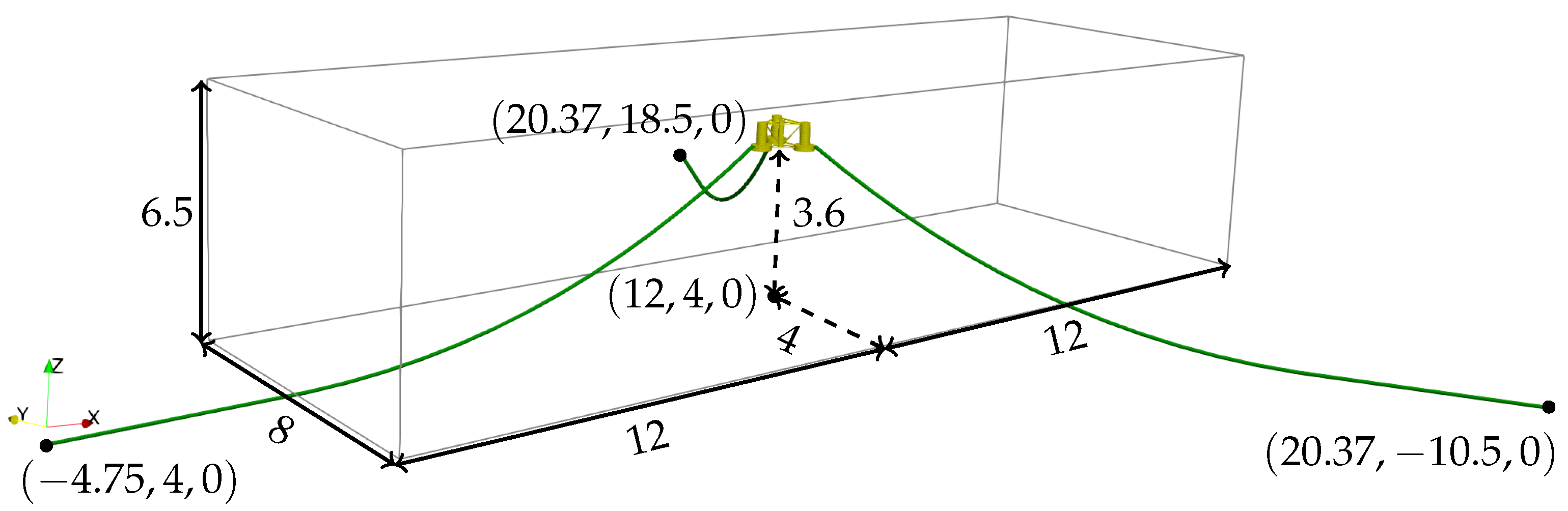
The chosen design was the well-established DeepCwind OC4 semi-submersible FOWT [52] at a 1:50 Froude scale taken from [53]. The sub-structure consists of three vertical columns connected to a more slender central column using multiple thin braces. Heave plates are attached to the bottom of the columns to increase stability. The platform is held in place through a mooring system consisting of three catenary lines spread symmetrically about the vertical axis of the structure. The fairleads of the lines are attached to the top of the heave plates, whereas the bottom ends of the lines lie on the sea ground. The stiffness matrices required for the present model were calculated from the given information about the elasticity module and second moments of area calculated from the assumption of a cylindrical shape. The reference solution was taken as the mean of the various numerical models presented in [54].

The structure was placed in the middle of a numerical wave tank, as shown in Figure 13. The tank had a length of 24 m, a width of 8 m and a height of $6.5$ m, and the water depth was 4 m. It can be noticed that the lower part of the mooring system was placed outside the computational domain to lower the computational costs of the simulations. This is also justified by the observation that the fluid velocities close to the bottom of the tank are small and a large portion of the mooring lines lies on the ground. Thus, the fluid velocities outside the computational domain but needed for the external force calculation of the mooring system were assumed to be zero. 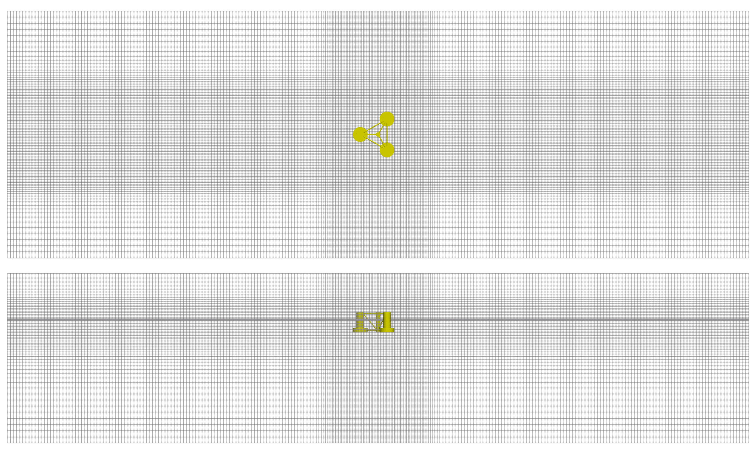Near the inlet of the domain, a wave generation zone was defined using the relaxation method [31]. A numerical beach at the end of the domain damped the wave energy to avoid reflections. A rectilinear grid was used to discretise the numerical domain. As can be seen in Figure 14, a refinement box with uniform grid sizes was defined around the structure. Cells of linearly increasing size were placed between the box and the domain boundaries to ensure a smooth transition. The grid size in the inner domain was determined from decay tests in heave and surge, presented next.

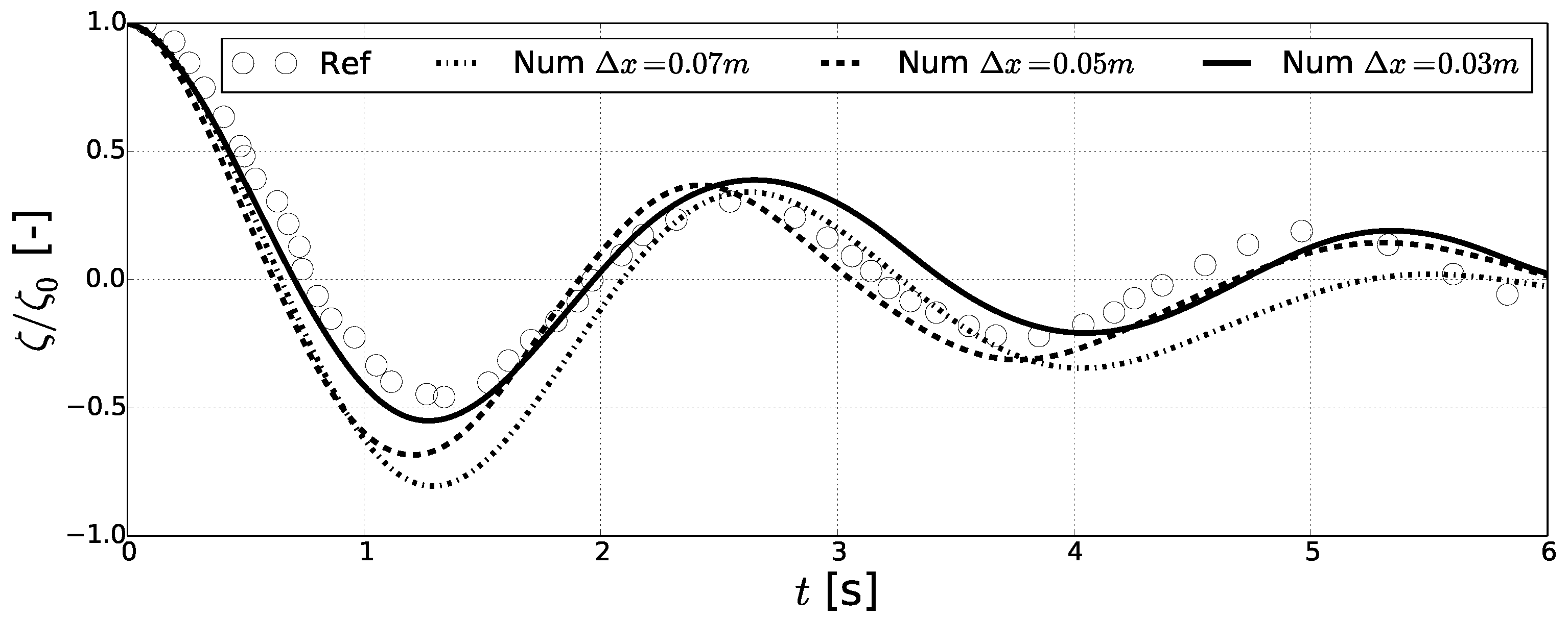
At first, a free heave decay test was conducted for the moored structure using three different grid sizes in the refinement box. The grid size outside of this inner region was automatically calculated based on linear grid growth with a ratio of $1.1$. Figure 15 presents the time series of the heave motion in comparison to the numerical solution in [54]. At the first peak after $1.2$ s, the numerical solution converged towards the reference, whereas all grids predicted the correct amplitude at the subsequent peaks. Further, the present model tended to predict a slightly longer natural period than the reference. 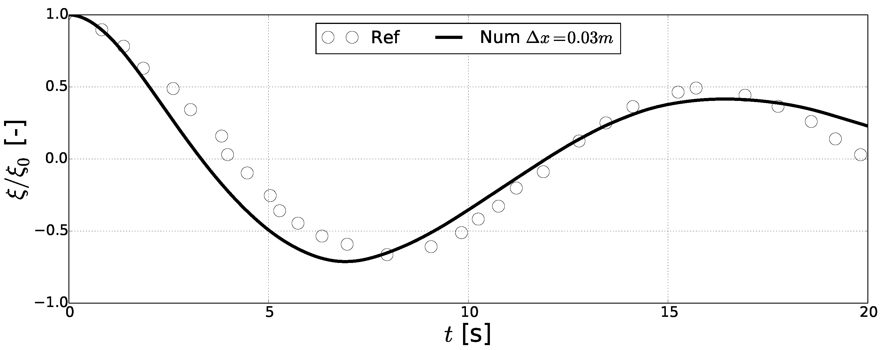Next, the grid with a minimum distance of $0.03$ m was chosen for the surge decay test (Figure 16). Both the amplitudes and the frequency of the motion were well predicted by the model. Therefore, this grid size was also used for the simulations below. The corresponding mesh had approximately $4.7$ million grid points.

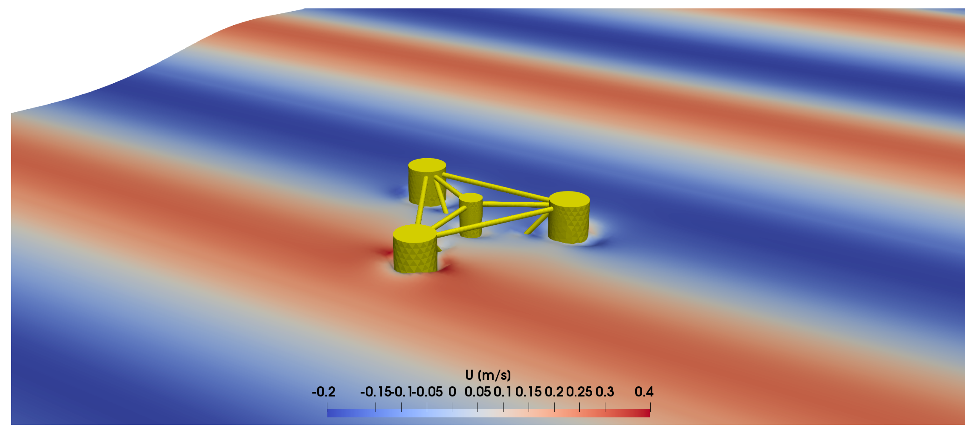
The accuracy of the numerical setup was assessed using a regular wave case with a wave height of $H=0.12$ m and a wave period of $T=1.41$ s. This corresponds to a wave length approximately twice the structural length, as can be seen in Figure 17. The wave was modelled as a second-order Stokes wave in the simulation.

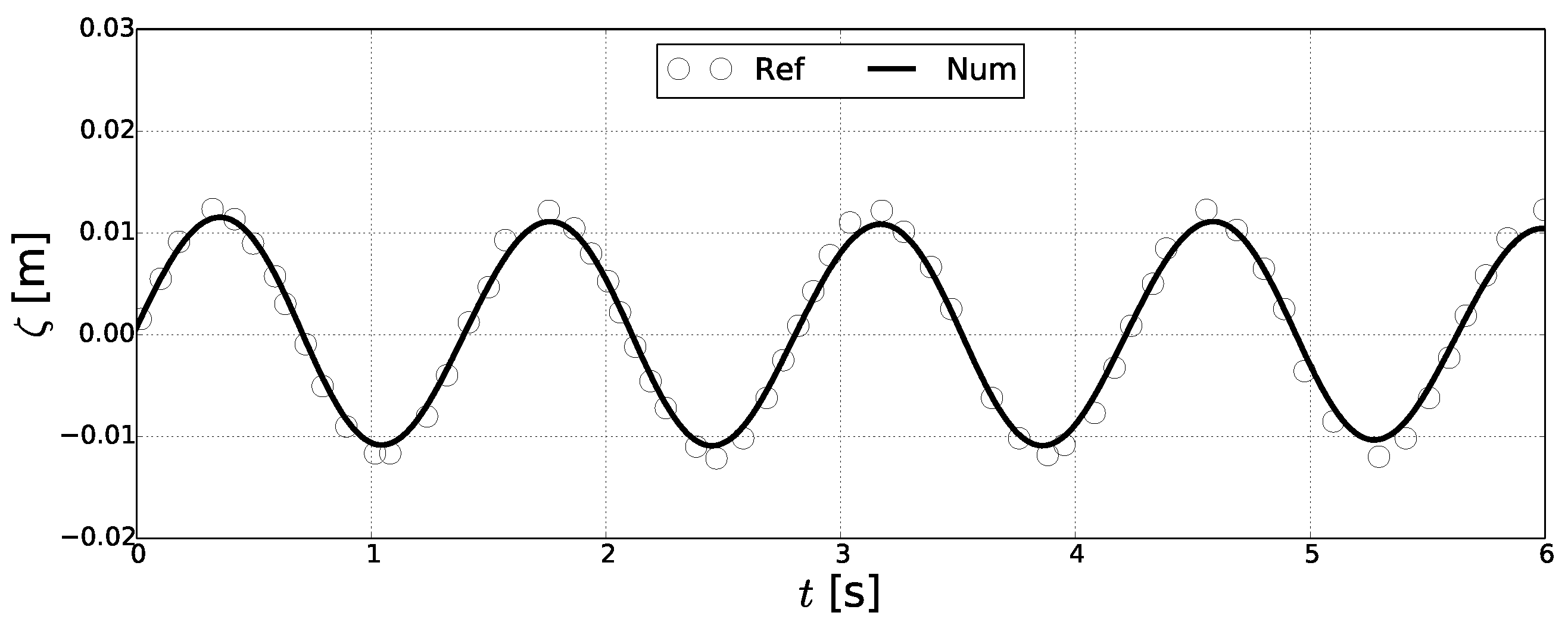
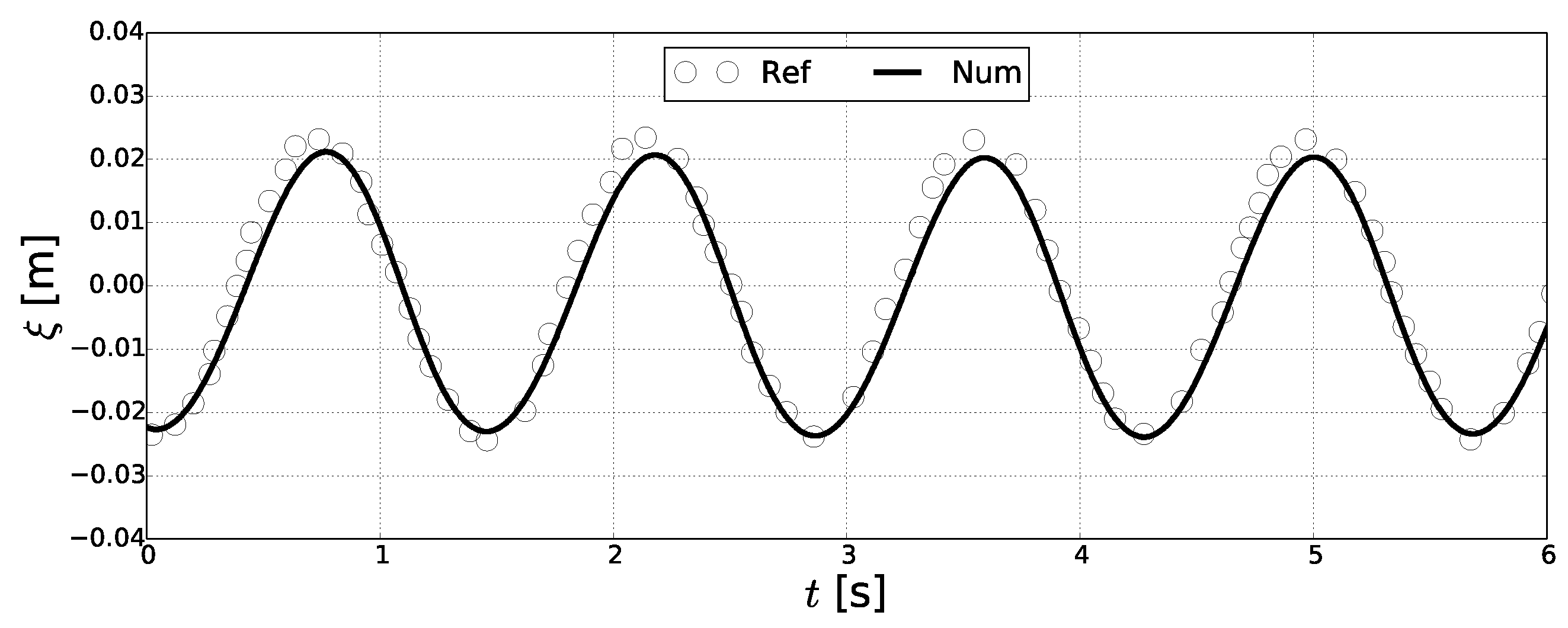
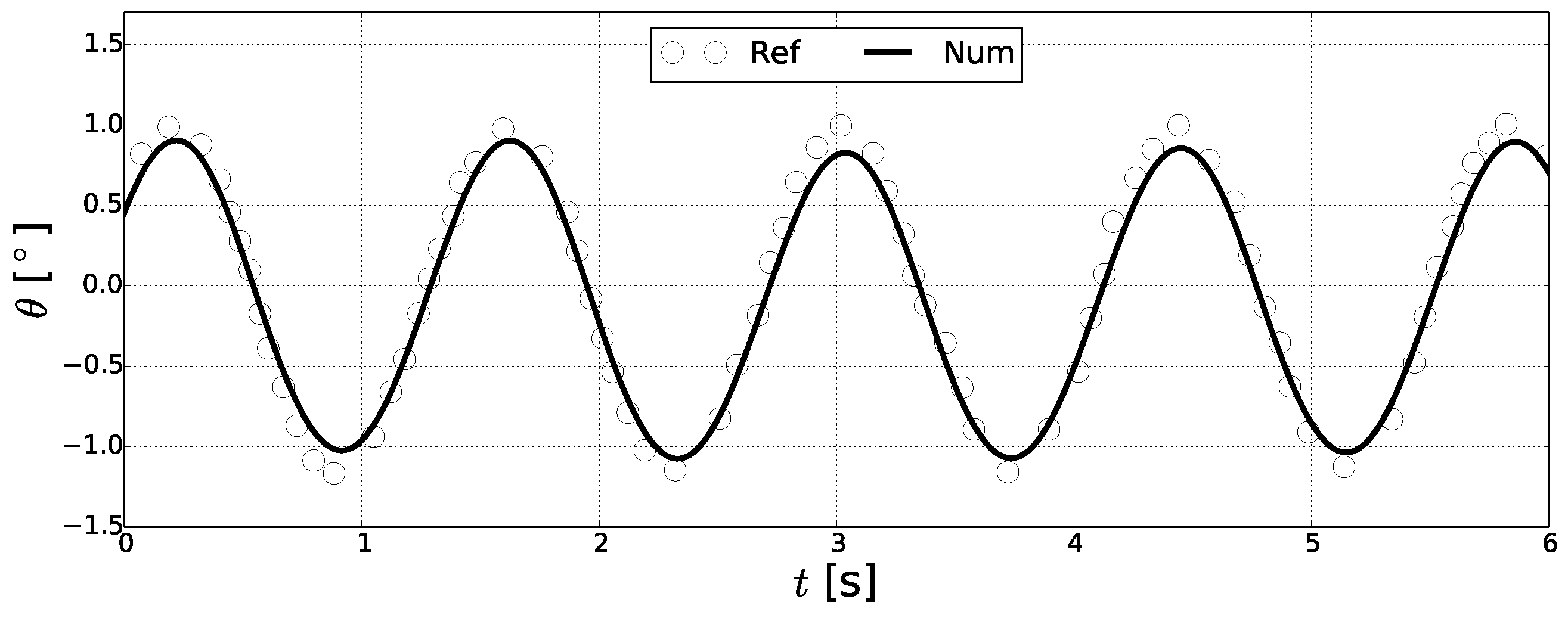
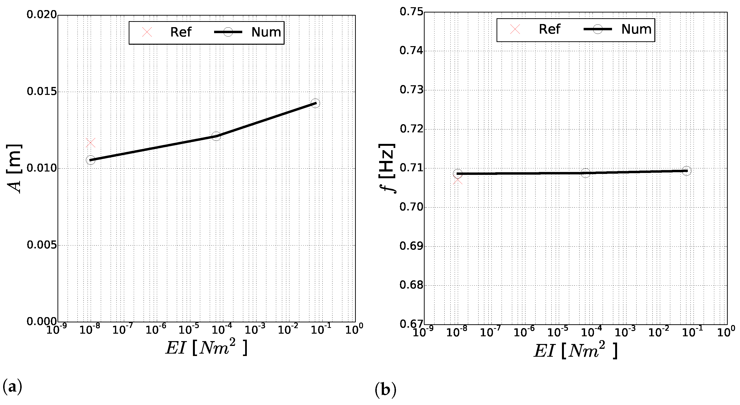
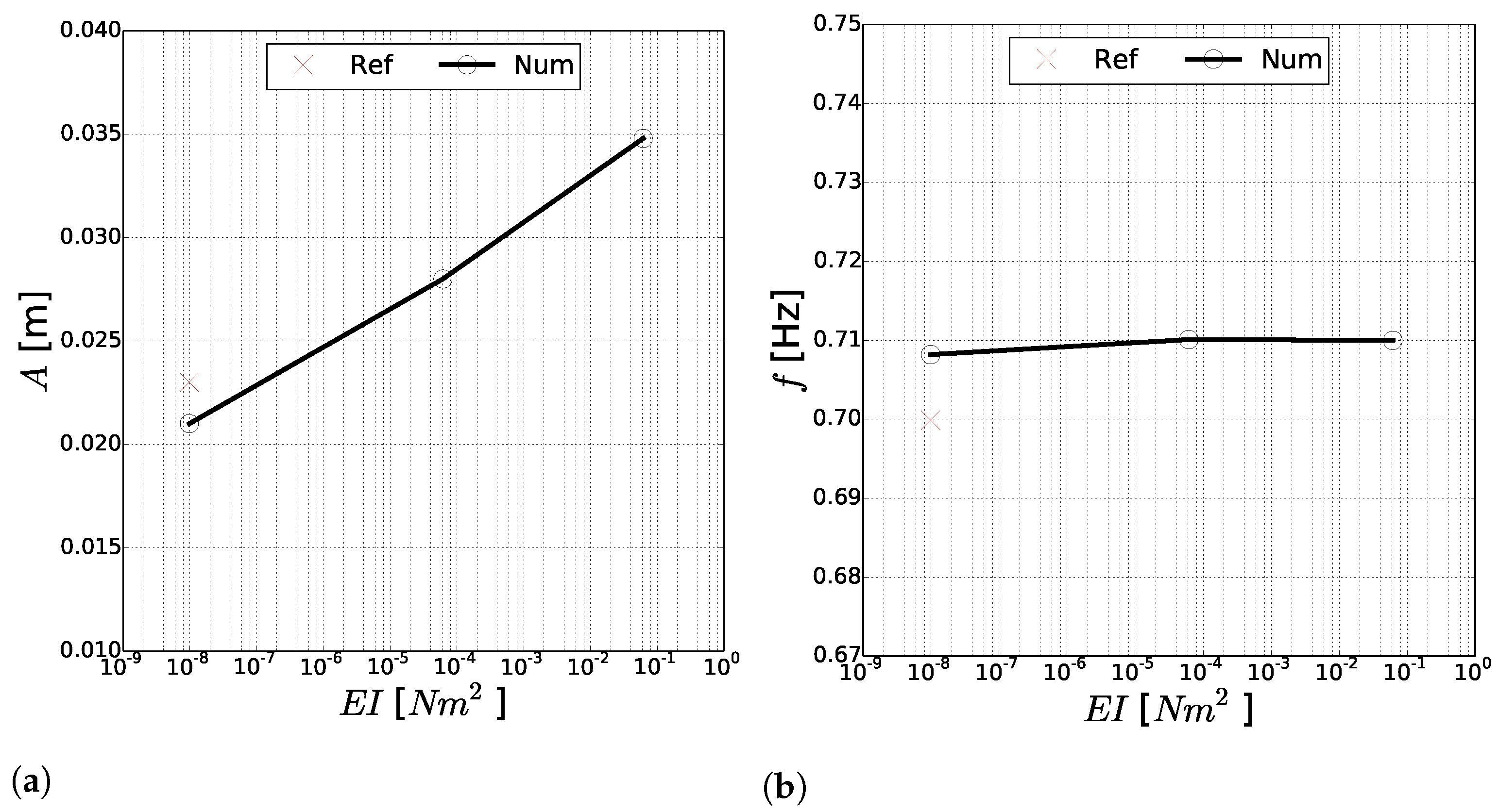
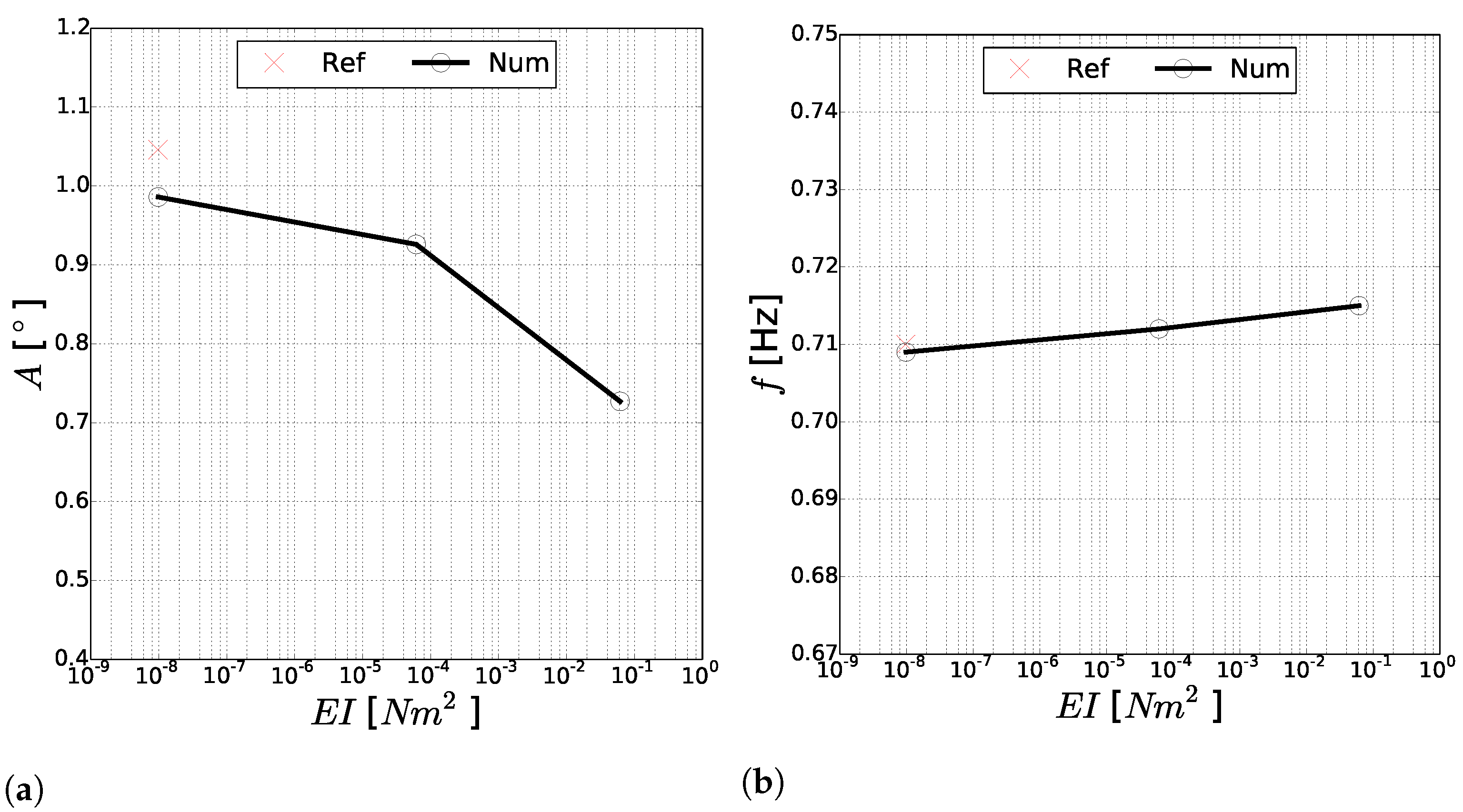
The qualitative comparison of the three body motions to the reference solution can be found in Figure 18, Figure 19 and Figure 20, whereas the quantification of the mean amplitude and frequency is shown in Figure 21, Figure 22 and Figure 23. The latter parameters were found from fast Fourier transformations of the steady-state time signals of the motions. Generally, good agreement between the presented and reference simulation can be stated. 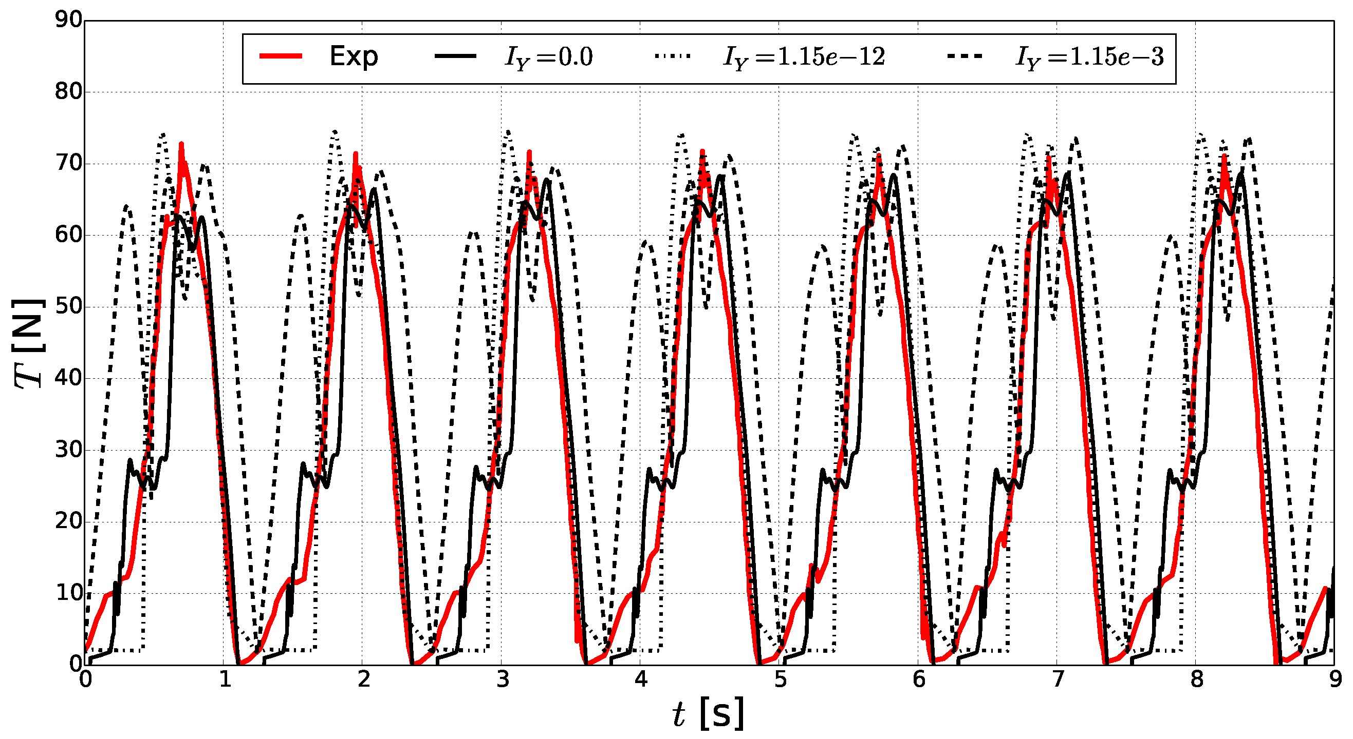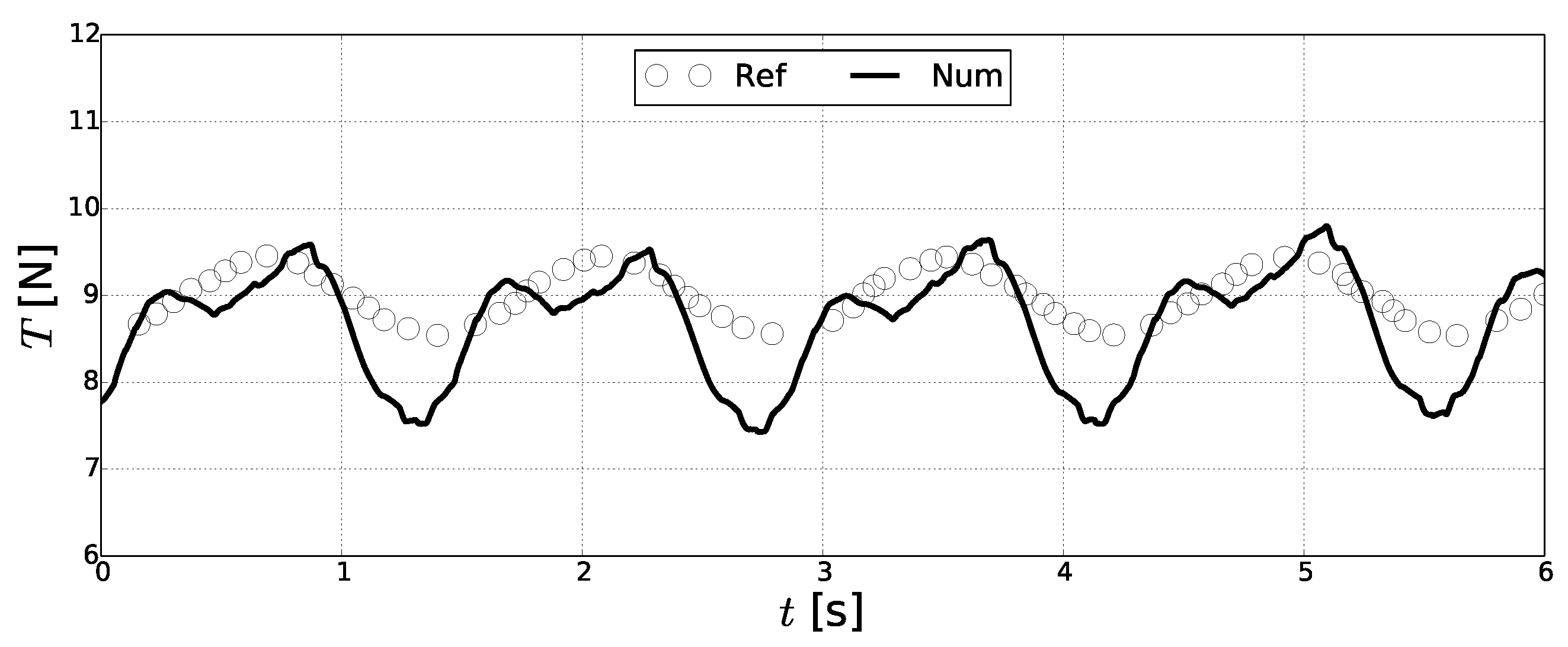The frequencies of the three motions are close to the encountered wave frequency of $0.71$ Hz. Further, the investigated model predicted lower motion amplitudes for the positive peaks. This is particularly prevalent for the surge motion, which indicates that the front mooring line might have caused this difference. The time series of the tension force magnitudes at the fairlead of the front mooring line is presented in Figure 24 to investigate this. In comparison to the reference solution, similar frequencies and crests of the forces but lower force troughs were predicted. This difference might be the reason for the slightly different motions of the structure.

Further insights into the influence of bending stiffness on the motion of moored, floating structures was provided by additional simulations with increased stiffness values. Figure 21, Figure 22 and Figure 23 present the amplitudes and frequencies of the motions for different bending stiffnesses. The reference solution from above, which is only available for the original bending stiffness, is also shown for comparison’s sake. It was first noticed that the frequencies of the heave and surge motions seem not to have been influenced by the increased stiffness. In contrast, the amplitudes of these motions increased by up to $40\%$ and $70\%$ respectively, and the pitch amplitude decreased by up to $30\%$. The reason for this was the additional rotational momentum, which restrained the rotation of the structure. Thus, the wave energy was rather converted into the translational modes. This also involved an increase of the mooring tension forces. It was finally observed that the bending stiffness led to an increased pitch frequency due to the larger system stiffness.

6. Conclusions

A new approach for simulating the dynamics of mooring systems and their interactions with floating structures was presented in this paper. It was based on a geometrically exact beam model originally developed for slender flexible rods. An efficient solution for the arising system of equations was found from a quaternion description of the rotational deformations and a finite difference discretisation. Explicit time integration was utilised, in contrast to previous approaches. The fluid forces acting on the system were calculated from Morison’s formula and the assumption of hydrodynamic transparency. The resulting mooring model has the advantage over existing models that it can account not just for bending but also shearing and torsion effects. Several verification and validation cases showed that the model is of second-order accuracy and can accurately represent the structural deformations and tension force distributions of rods and mooring lines.

The mooring model was then coupled to a two-phase CFD solver to investigate moored, floating structures in waves. The applicability of this approach was shown for the semi-submersible floating offshore wind support structure of the DeepCwind OC4 project. Initial decay tests in heave and surge were conducted to study the convergence of the numerical model and determine the required number of grid points. Then, the motion of the structure in a regular wave was compared to previous numerical solutions. Good agreement for the amplitude and frequency of the heave, surge and pitch motion was shown. A study of the influences of increasing bending stiffness on these motions revealed only a minor change to the motion frequencies but significant effects on the amplitudes. The additional rotational momentum decreased the rotation of the structure so that the wave energy acted more strongly on the translational modes.

The presented development of a dynamic mooring model is only one possible application for geometrically exact beam theory. Within further research, the same model will be applied to other slender marine structures, such as monopiles, offshore wind turbine towers and floaters. Additionally, electrical submarine cables might be of interest, as they do not only experience axial elongation but also torsion in the helical armour [55]. Further, the comparison to the analytical solution for the forced vibration of a pinned rod revealed a principal deviation of the chosen numerical approach. Previous research showed better results using finite element methods. Within further developments, it has to be investigated what causes the problems of the finite difference discretisation and whether the deviations can be avoided by switching to a finite element solution.

References

1. Faltinsen, O. Sea Loads on Ships and Offshore Structures; Cambridge University Press: Cambridge, UK, 1990. [Google Scholar]
2. Martin, T.; Kamath, A.; Bihs, H. Modelling and Simulation of Moored-floating Structures using the Tension-Element-Method. In Proceedings of the ASME 2018 37th International Conference on Ocean, Offshore and Arctic Engineering, Madrid, Spain, 17–22 June 2018; Volume 2. [Google Scholar]
3. Martin, T.; Kamath, A.; Bihs, H. Accurate modelling of the interaction of constrained floating structures and complex free surfaces using a new quasi-static mooring model. Int. J. Numer. Meth. Fluids 2021, 93, 504–526. [Google Scholar] [CrossRef]
4. Ablow, C.; Schechter, S. Numerical Solution of Undersea Cable Dynamics. Ocean Eng. 1983, 10, 443–457. [Google Scholar] [CrossRef]
5. Mavrakos, S.; Papazoglou, V.; Triantafyllou, M.; Hatjigeorgiou, J. Deep water mooring dynamics. Mar. Struct. 1996, 9, 181–209. [Google Scholar] [CrossRef]
6. Gobat, J.; Grosenbaugh, M. Dynamics in the trouchdown region of catenary moorings. In Proceedings of the 11th International Offshore and Polar Engineering Conference, Stavanger, Norway, 17–22 June 2001. [Google Scholar]
7. Aamo, O.; Fossen, T. Finite Element Modelling of Moored Vessels. Math. Comput. Model. Dyn. Syst. 2001, 7, 47–75. [Google Scholar] [CrossRef]
8. Buckham, B.; Driscoll, F.R.; Nahon, M. Development of a Finite Element Cable Model for Use in Low-Tension Dynamics Simulation. J. Appl. Mech. 2004, 71, 476–485. [Google Scholar] [CrossRef]
9. Garrett, D.L. Dynamic Analysis of Slender Rods. J. Energy Resour. Technol. 1982, 104, 302–306. [Google Scholar] [CrossRef]
10. Walton, T.; Polachek, H. Calculation of transient motion of submerged cables. Math. Comp. 1959, 14, 27–46. [Google Scholar] [CrossRef]
11. Vissio, G.; Passione, B.; Hall, M.; Raffero, M. Expanding ISWEC Modelling with a Lumped-Mass Mooring Line Model. In Proceedings of the European Wave and Tidal Energy Conference, Nantes, France, 6–11 September 2015. [Google Scholar]
12. Hall, M.; Goupee, A. Validation of a lumped-mass mooring line model with DeepCwind semisubmersible model test data. Ocean Eng. 2015, 104, 590–603. [Google Scholar] [CrossRef] [Green Version]
13. Palm, J.; Eskilsson, C.; Bergdahl, L. An hp-adaptive discontinuous Galerkin method for modelling snap loads in mooring cables. Ocean Eng. 2017, 144, 266–276. [Google Scholar] [CrossRef]
14. Palm, J.; Eskilsson, C. Influence of Bending Stiffness on Snap Loads in Marine Cables: A Study Using a High-Order Discontinuous Galerkin Method. J. Mar. Sci. Eng. 2020, 8, 795. [Google Scholar] [CrossRef]
15. Zhu, Z.; Meguid, S. Elastodynamic Analysis of Low Tension Cables Using a New Curved Beam Element. Int. J. Solids Struct. 2006, 43, 1490–1504. [Google Scholar] [CrossRef] [Green Version]
16. Burgess, J. Bending Stiffness in a Simulation of Undersea Cable Deployment. Int. J. Offshore Polar Eng. 1993, 3, 197–204. [Google Scholar]
17. Tjavaras, A. The Dynamics of Highly Extensible Cables. Ph.D. Thesis, MIT, Cambridge, MA, USA, 1996. [Google Scholar]
18. Cottanceau, E.; Thomas, O.; Véron, P.; Alochet, M.; Deligny, R. A Finite Element/Quaternion/Asymptotic Numerical Method for the 3D Simulation of Flexible Cables. Finite Elem. Anal. Des. 2018, 139, 14–34. [Google Scholar] [CrossRef] [Green Version]
19. Lang, H.; Arnold, M. Numerical aspects in the dynamic simulation of geometrically exact rods. Appl. Numer. Math. 2012, 62, 1411–1427. [Google Scholar] [CrossRef]
20. Antman, S. Kirchhoff’s problem for nonlinearly elastic rods. Quart. J. Appl. Math 1974, 32, 221–240. [Google Scholar] [CrossRef] [Green Version]
21. Reissner, E. On finite deformations of space-curved beams. Z. Angew. Math. Phys. ZAMP 1981, 32, 734–744. [Google Scholar] [CrossRef]
22. Cosserat, E.; Cosserat, F. Théorie des Corps dé Formables. Librairie Scientifique A. Hermann et Fils (Translation: Theory of Deformable Bodies, NASA TT F-11 561, 1968). 1909. Available online: https://www.worldcat.org/title/theory-of-deformable-bodies/oclc/641300962 (accessed on 29 April 2021).
23. Simo, J. A finite strain beam formulation. The three-dimensional dynamic problem. Part I. Comput. Meth. Appl. Mech. Eng. 1985, 49, 55–70. [Google Scholar] [CrossRef]
24. Simo, J.; Vu-Quoc, L. On the dynamics of flexible beams under large overall motions—the plane case: Part II. J. Appl. Mech. 1986, 53, 855–863. [Google Scholar] [CrossRef]
25. Simo, J.; Vu-Quoc, L. On the dynamics in space of rods undergoing large motions—A geometrically exact approach. Comput. Methods Appl. Mech. Eng. 1988, 66, 125–161. [Google Scholar] [CrossRef]
26. Quan, W.; Chang, Q.; Zhang, Q.; Gong, J. Dynamics Calculation for Variable-Length Underwater Cable with Geometrically Nonlinear Motion. Ocean Eng. 2020, 212, 107695. [Google Scholar] [CrossRef]
27. Zupan, E.; Saje, M.; Zupan, D. Dynamics of spatial beams in quaternion description based on the Newmark integration scheme. Comput. Mech. 2013, 51, 47–64. [Google Scholar] [CrossRef]
28. Weeger, O.; Yeung, S.K.; Dunn, M.L. Isogeometric Collocation Methods for Cosserat Rods and Rod Structures. Comput. Methods Appl. Mech. Eng. 2017, 316, 100–122. [Google Scholar] [CrossRef]
29. Lang, H.; Arnold, M. Multibody dynamics simulation of geometrically exact Cosserat rods. Multibody Syst. Dyn. 2011, 25, 285–312. [Google Scholar] [CrossRef]
30. Tschisgale, S.; Fröhlich, J. An immersed boundary method for the fluid-structure interaction of slender flexible structures in viscous fluid. J. Comput. Phys. 2020, 423. [Google Scholar] [CrossRef]
31. Bihs, H.; Kamath, A.; Alagan Chella, M.; Aggarwal, A.; Arntsen, Ø.A. A new level set numerical wave tank with improved density interpolation for complex wave hydrodynamics. Comput. Fluids 2016, 140, 191–208. [Google Scholar] [CrossRef]
32. Shu, C.; Osher, S. Efficient implementation of essentially non-oscillatory shock-capturing schemes. J. Comput. Phys. 1988, 77, 439–471. [Google Scholar] [CrossRef] [Green Version]
33. Shoemake, K. Animating Rotation with Quaternion Curves. SIGGRAPH Comput. Graph. 1985, 19, 245–254. [Google Scholar] [CrossRef]
34. Tschisgale, S. A Numerical Method for Fluid-Structure Interactions of Slender Rods in Turbulent Flow. Ph.D. Thesis, TUDpress, Dresden, Germany, 2020. [Google Scholar]
35. Morison, J.; O’Brien, M.; Johnson, J.; Schaaf, S. The force exerted by surface waves on piles. Pet. Trans. Amer. Inst. Min. Eng. 1950, 186, 149–154. [Google Scholar] [CrossRef]
36. Martin, T.; Schacht, S.; Riesen, P.; Paschen, M. Efficient implementation of a numerical model for flexible net structures. Ocean Eng. 2018, 150, 272–279. [Google Scholar] [CrossRef]
37. Choo, Y.I.; Casarella, M. Hydrodynamic Resistance of Towed Cables. J. Hydronautics 1971, 5, 126–131. [Google Scholar]
38. Martin, T.; Bihs, H. A non-linear implicit approach for modelling the dynamics of porous tensile structures interacting with fluids. J. Fluids Struct. 2021, 100. [Google Scholar] [CrossRef]
39. Osher, S.; Sethian, J. Fronts propagating with curvature-dependent speed: Algorithms based on Hamilton-Jacobi formulations. J. Comput. Phys. 1988, 79, 12–49. [Google Scholar] [CrossRef] [Green Version]
40. Sussman, M.; Smereka, P.; Osher, S. A level set approach for computing solutions to incompressible two-phase flow. J. Comput. Phys. 1994, 114, 146–159. [Google Scholar] [CrossRef]
41. Martin, T.; Tsarau, A.; Bihs, H. A numerical framework for modelling the dynamics of open ocean aquaculture structures in viscous fluids. Appl. Ocean. Res. 2021, 106. [Google Scholar] [CrossRef]
42. Timmermans, L.; Minev, P.; Van De Vosse, F. An approximate projection scheme for incompressible flow using spectral elements. Int. J. Numer. Methods Fluid 1996, 22, 673–688. [Google Scholar] [CrossRef]
43. Jiang, G.; Peng, D. Weighted ENO schemes for Hamilton Jacobi equations. SIAM J. Sci. Comput. 2000, 21, 2126–2143. [Google Scholar] [CrossRef] [Green Version]
44. Jiang, G.; Shu, C. Efficient implementation of weighted ENO schemes. J. Comput. Phys. 1996, 12, 202–228. [Google Scholar] [CrossRef] [Green Version]
45. Palm, J. Mooring Dynamics for Wave Energy Applications. Ph.D. Thesis, Chalmers University of Technology, Gothenburg, Sweden, 2017. [Google Scholar]
46. Bathe, K.J.; Bolourchi, S. Large displacement analysis of three-dimensional beam structures. Int. J. Numer. Meth. 1979, 14, 961–986. [Google Scholar] [CrossRef]
47. Rao, S.S. Vibration of Continuous Systems; John Wiley & Sons, Inc.: Hoboken, NJ, USA, 2007. [Google Scholar]
48. Hesse, H.; Palacios, R. Consistent structural linearisation in flexible-body dynamics with large rigid-body motion. Comput. Struct. 2012, 110–111, 1–14. [Google Scholar] [CrossRef] [Green Version]
49. Koh, C.; Zhang, Y.; Quek, S. Low-tension cable dynamics: Numerical and experimental studies. J. Eng. Mech. 1999, 125, 347–354. [Google Scholar] [CrossRef]
50. Lockwood, E. A Book of Curves; Cambridge University Press: Cambridge, UK, 1961. [Google Scholar]
51. Bergdahl, L.; Palm, J.; Eskilsson, C.; Lindahl, L. Dynamically scaled model experiment of a mooring cable. J. Mar. Sci. Technol. 2016, 4, 5. [Google Scholar] [CrossRef] [Green Version]
52. Robertson, A.; Jonkman, J.; Masciola, M.; Song, H.; Goupee, A.; Coulling, A.; Luan, C. Definition of the Semisubmersible Floating System for Phase II of OC4. Tech. Rep. 2014. [Google Scholar] [CrossRef] [Green Version]
53. Bruinsma, N. Validation and Application of a Fully Nonlinear Numerical WaveTank. Master’s Thesis, Technical University of Delft, Delft, The Netherlands, 2016. [Google Scholar]
54. Robertson, A.; Jonkman, J.; Vorpahl, F.; Popko, W.; Qvist, J.; Froyd, L.; Chen, X.; Azcona, J.; Uzungoglu, E.; Guedes Soares, C.; et al. Offshore Code Comparison Collaboration, Continuation within IEA Wind Task 30: Phase II Results Regarding a Floating Semisubmersible Wind System: Preprint. Tech. Rep. 2014. [Google Scholar] [CrossRef]
55. Chang, H.C.; Chen, B.F. Mechanical Behavior of Submarine Cable under Coupled Tension, Torsion and Compressive Loads. Ocean Eng. 2019, 189, 106272. [Google Scholar] [CrossRef]
Figure 1. Definition of the discrete rod line (solid line) using N bluesegments of length Δ X . The bluesegment edges are marked as points, the segment centres as bars. The (dashed lines) show the ghost point extensions at both ends of the rod.
Jmse 09 00486 g001
Figure 2. Flowchart of the algorithm to simulate the fluid–structure interaction of moored, floating structures in waves.
Jmse 09 00486 g002
Figure 3. Convergence of the L2 norm of error for the end position of the deformed rod. The solution for N = 320 is taken as the exact solution here. The red line corresponds to a convergence rate of p = 2. (a) Case with a 3 N load. (b) Case with a 6 N load.
Jmse 09 00486 g003
Figure 4. Convergence study for the angle a of the rigid pendulum in a gravity field. (a) Differences of the angle between the numerical solutions with N = 10 to N = 80 and the theoretical solution over two periods. (b) Spatial convergence of the L2 norms of error. The red lines correspond to convergence rates of p = 1 and 2.
Jmse 09 00486 g004
Figure 5. Comparison of the numerical and theoretical solutions for the vibration of a pinned rod under static force excitation.
Jmse 09 00486 g005
Figure 6. Motion of the free-free flexible rod for the two-dimensional load case. The red line shows the initial position of the rod. The reference solution was taken from [48].
Jmse 09 00486 g006
Figure 7. Motion of the free-free flexible rod for the three-dimensional load case. The red lines show the initial position of the rod. The reference solution was taken from [48]. (a) Motion in the x-z plane. (b) Motion in the y-z plane.
Jmse 09 00486 g007
Figure 8. Deformation of a swinging elastic rod pinned at one end. The black lines show the deformed rod in 0.1 s time increments. The red line shows the initial position of the rod.
Jmse 09 00486 g008
Figure 9. Tension force distribution over time at two different positions for the swinging elastic rod.
Jmse 09 00486 g009
Figure 10. Tension force distribution over time close to the pin for the swinging elastic hanging rod.
Jmse 09 00486 g010
Figure 11. Numerically predicted fairlead tension force magnitudes in comparison to the experimental results. (a) T = 1.25 s. (b) T = 3.5 s.
Jmse 09 00486 g011
Figure 12. Numerically predicted fairlead tension force magnitudes for different bending stiffnesses in comparison to the experimental results for T = 1.25 s.
Jmse 09 00486 g012
Figure 13. Computational domain and mooring system for the simulation of a moored, floating offshore wind turbine in waves.
Jmse 09 00486 g013
Figure 14. Computational grid for the simulation of a moored, floating offshore wind turbine in waves.
Jmse 09 00486 g014
Figure 15. Convergence of the numerical solution for the free heave decay test for the support structure. The numerical reference solution was taken from [54].
Jmse 09 00486 g015
Figure 16. Convergence of the numerical solution for the free surge decay test for the support structure. The numerical reference solution was taken from [54].
Jmse 09 00486 g016
Figure 17. Illustration of the support structure facing a wave crest. The contour shows the free surface, and the colours indicate the velocities in x direction.
Jmse 09 00486 g017
Figure 18. Numerical solution for the heave motion over time with regular waves. The numerical reference solution was taken from [54].
Jmse 09 00486 g018
Figure 19. Numerical solution for the surge motion over time with regular waves. The numerical reference solution was taken from [54].
Jmse 09 00486 g019
Figure 20. Numerical solution for the pitch motion over time with regular waves. The numerical reference solution was taken from [54].
Jmse 09 00486 g020
Figure 21. Parameter study of the effects of EI on the (a) amplitude and (b) frequency of the heave motion.
Jmse 09 00486 g021
Figure 22. Parameter study of the effects of EI on the (a) amplitude and (b) frequency of the surge motion.
Jmse 09 00486 g022
Figure 23. Parameter study of the effects of EI on the (a) amplitude and (b) frequency of the pitch motion.
Jmse 09 00486 g023
Figure 24. Numerical solution for the tension force magnitudes at the fairlead of the front mooring line over time with regular waves. The numerical reference solution was taken from [54].
Jmse 09 00486 g024