Author Contributions
G.G., C.J., F.S., T.D. and B.G.S. conceptualised and formulated the hypothesis. B.G., S.O.-S. and R.M. conducted the formal analysis. B.G., G.G. and J.-V.F. provided the experimental turbine model and measurement tools. B.G., J.-V.F., F.S., I.S. and C.O. performed the investigation process and experiments. B.G., S.O.-S. and G.G. developed the methodology. B.G., S.O.-S., R.M. and G.G. wrote the original draft. F.S., I.S., T.D. and C.O. reviewed and revised the published work. All authors have read and agreed to the published version of the manuscript.
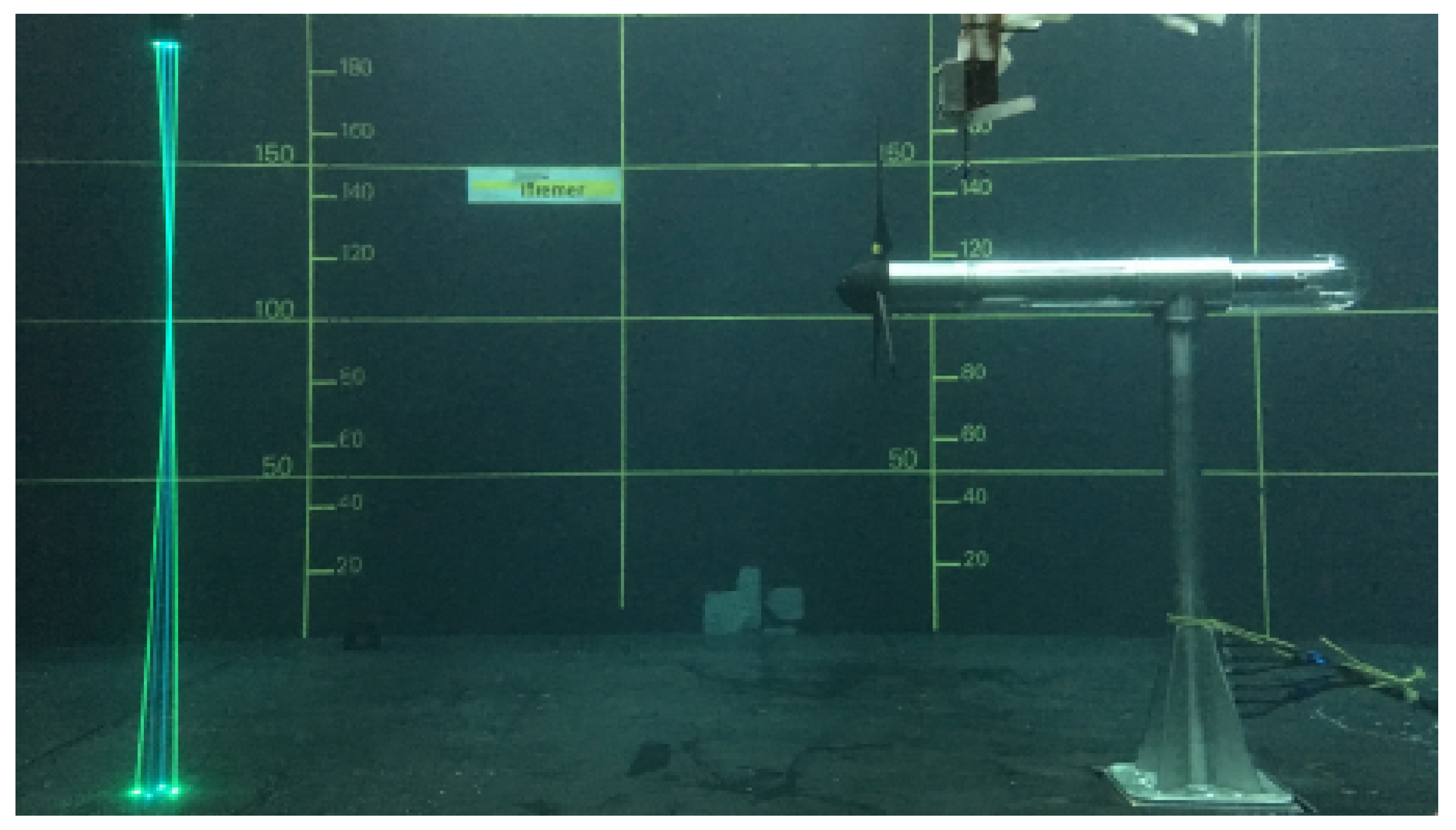
Figure 1.
Side view of the three-bladed instrumented turbine in the wave and current flume tank of Ifremer.
Figure 1.
Side view of the three-bladed instrumented turbine in the wave and current flume tank of Ifremer.
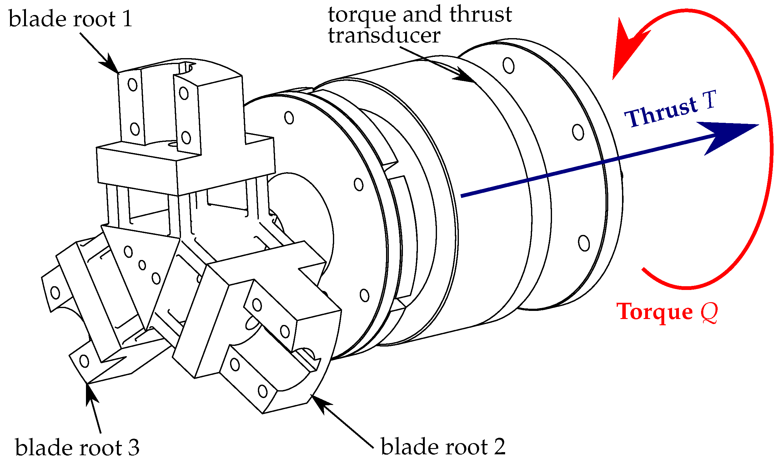
Figure 2.
The torque and thrust transducer.
Figure 2.
The torque and thrust transducer.
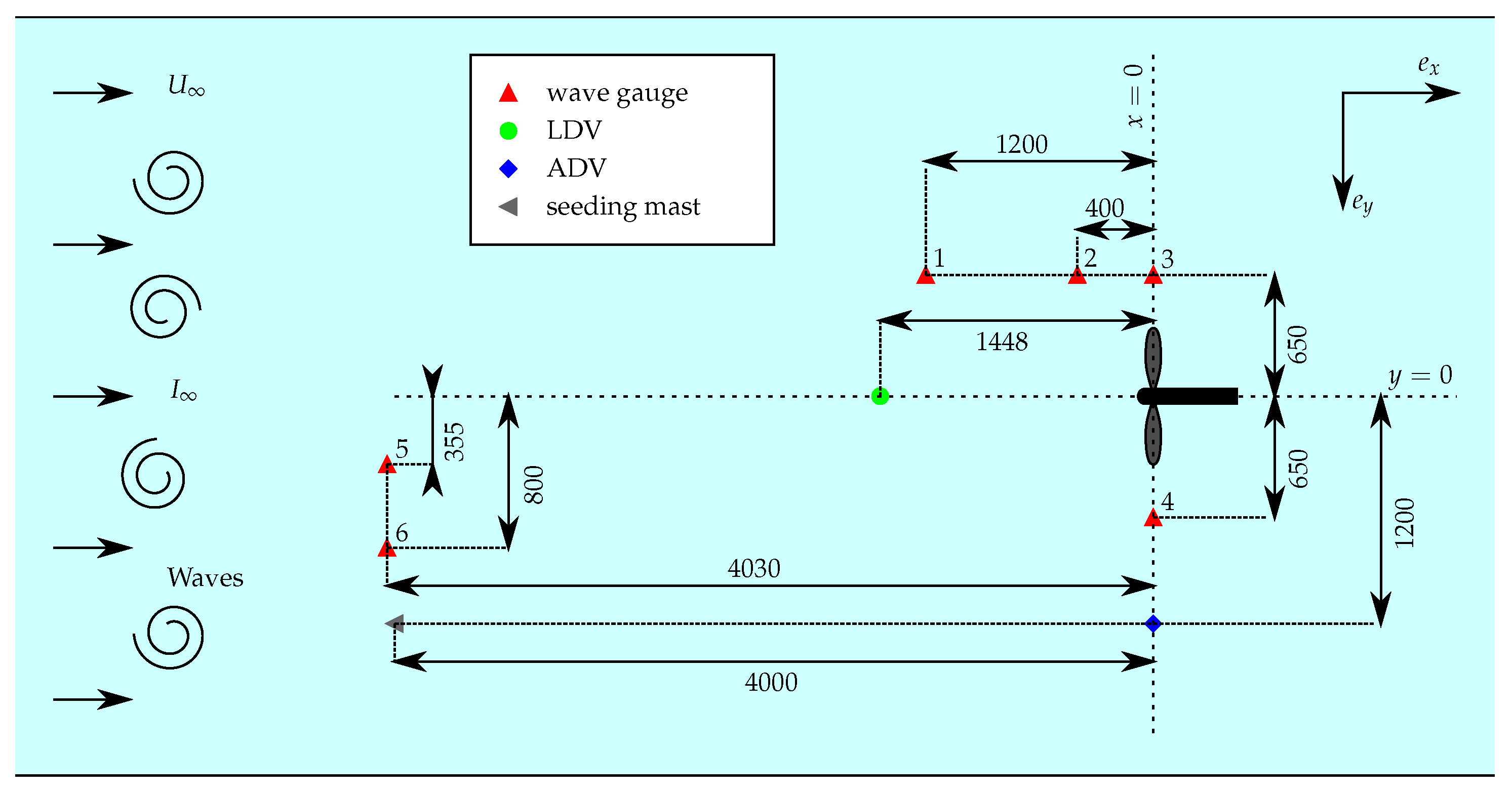
Figure 3.
Schematic top-view of the test set-up used in the three tanks. The ADV is used at Ifremer, FloWave and Cnr-Inm. The LDV is only used at Ifremer. The seeding mast is required at Cnr-Inm only. The wave gauges 1 to 3 are used at Ifremer and FloWave and 3 to 6 at Cnr-Inm. Dimensions are given in and the presented tank width represents the Ifremer size.
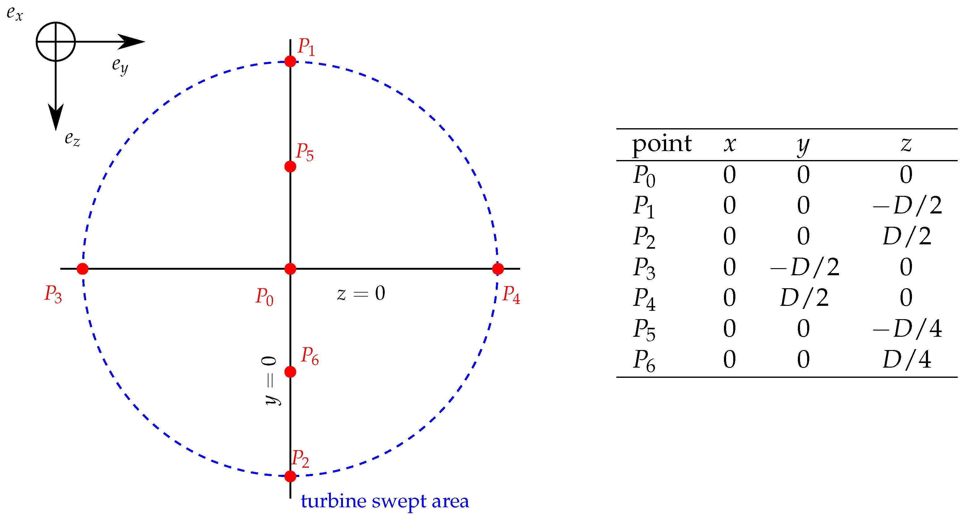
Figure 4.
Front view of the ADV measurement points describing the swept area of the turbine and their coordinates expressed in diameter . Points 0 to 2 and 5 and 6 are acquired at Ifremer. Points 0 to 2 are acquired at Cnr-Inm. Points 0 to 4 are acquired at FloWave.
Figure 4.
Front view of the ADV measurement points describing the swept area of the turbine and their coordinates expressed in diameter . Points 0 to 2 and 5 and 6 are acquired at Ifremer. Points 0 to 2 are acquired at Cnr-Inm. Points 0 to 4 are acquired at FloWave.
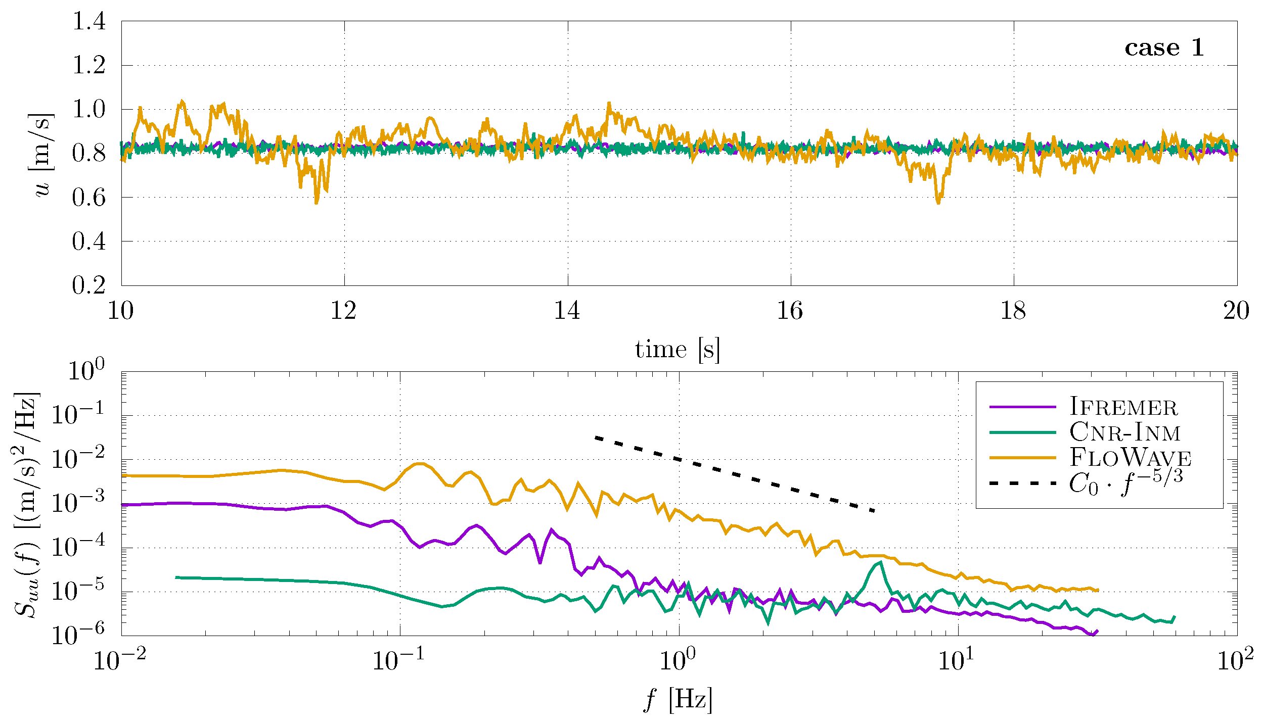
Figure 5.
Time histories (top) of the ADV streamwise velocity u measured at the top-dead centre of the rotor for case 1 and their corresponding PSD (bottom) at Ifremer, FloWave and Cnr-Inm. The PSD panel also includes Kolmogorov’s −5/3 power law.
Figure 5.
Time histories (top) of the ADV streamwise velocity u measured at the top-dead centre of the rotor for case 1 and their corresponding PSD (bottom) at Ifremer, FloWave and Cnr-Inm. The PSD panel also includes Kolmogorov’s −5/3 power law.
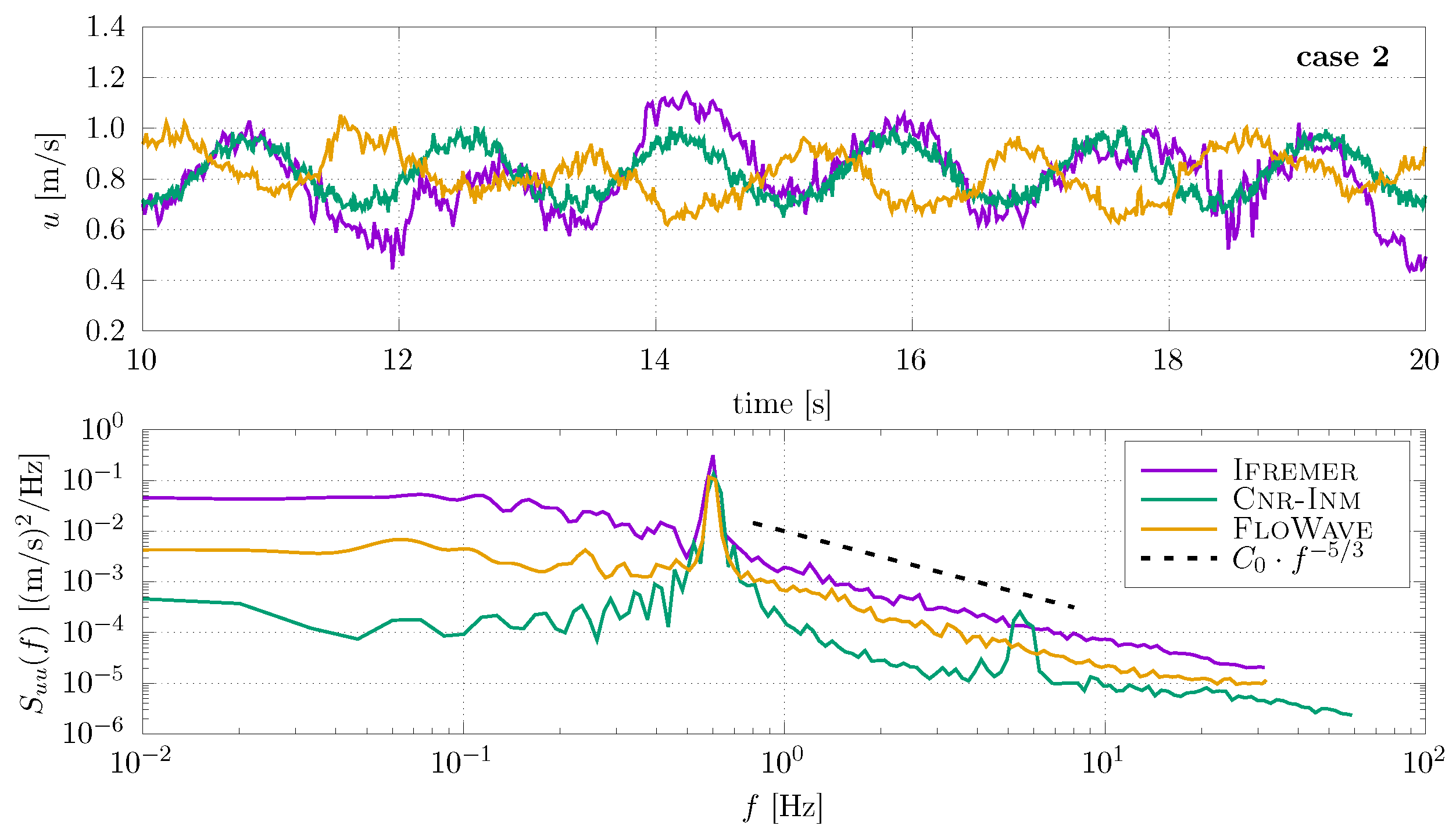
Figure 6.
Time histories (top) of the ADV streamwise velocity u measured at the top-dead centre of the rotor for case 2 and their corresponding PSD (bottom) at Ifremer, FloWave and Cnr-Inm. The PSD panel also includes Kolmogorov’s −5/3 power law.
Figure 6.
Time histories (top) of the ADV streamwise velocity u measured at the top-dead centre of the rotor for case 2 and their corresponding PSD (bottom) at Ifremer, FloWave and Cnr-Inm. The PSD panel also includes Kolmogorov’s −5/3 power law.
Figure 7.
Time average (markers) and standard deviation (shading) of the ADV stream-wise velocity u versus turbine rotational speed for current-only case 1 at all facilities. Dashed lines are the average of u for case 1 at all rotational speed settings per facility; the red line is the target value of 0.8 m/s.
Figure 8.
Time average (markers) and standard deviation (shading) of the ADV stream-wise velocity u measured in synchronisation with the turbine against turbine rotational speed for wave and current case 2 at all facilities. Dashed lines are the average of u for case 2 at all rotational speed settings per facility. Red line is the target value of 0.8 m/s.
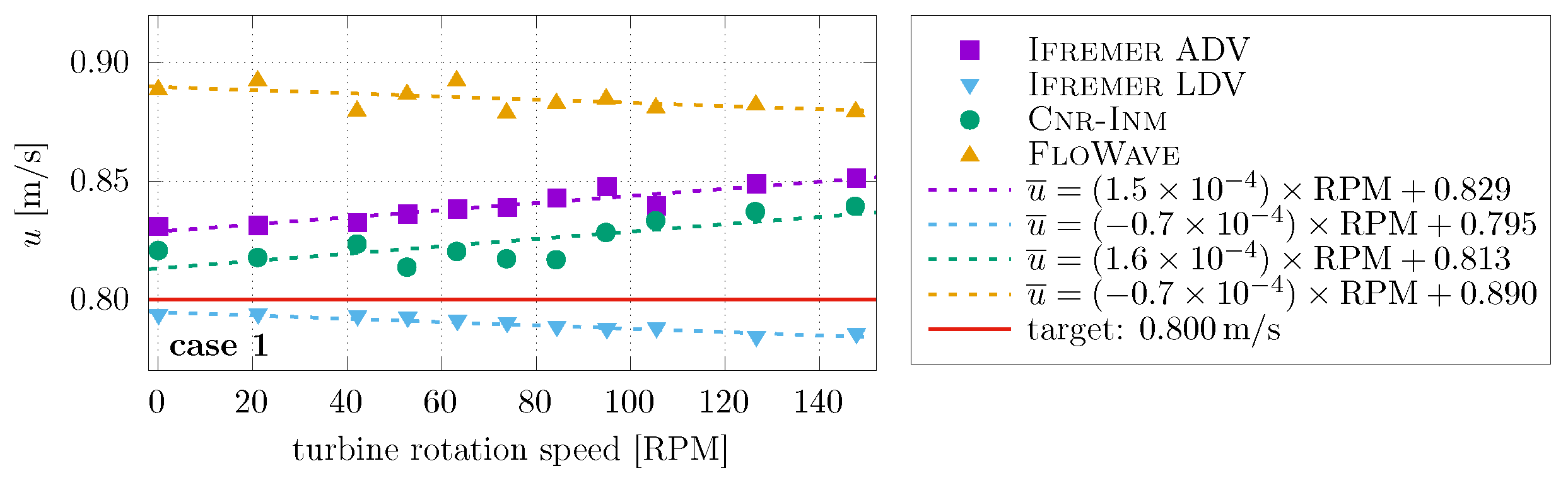
Figure 9.
Variation of the time-averaged (markers) and linear regression (dotted lines) of the ADV and LDV (only at Ifremer) stream-wise velocity u in synchronisation with the turbine against the turbine rotational speed for case 1 at all facilities. The red line indicates the target velocity of 0.8 m/s.
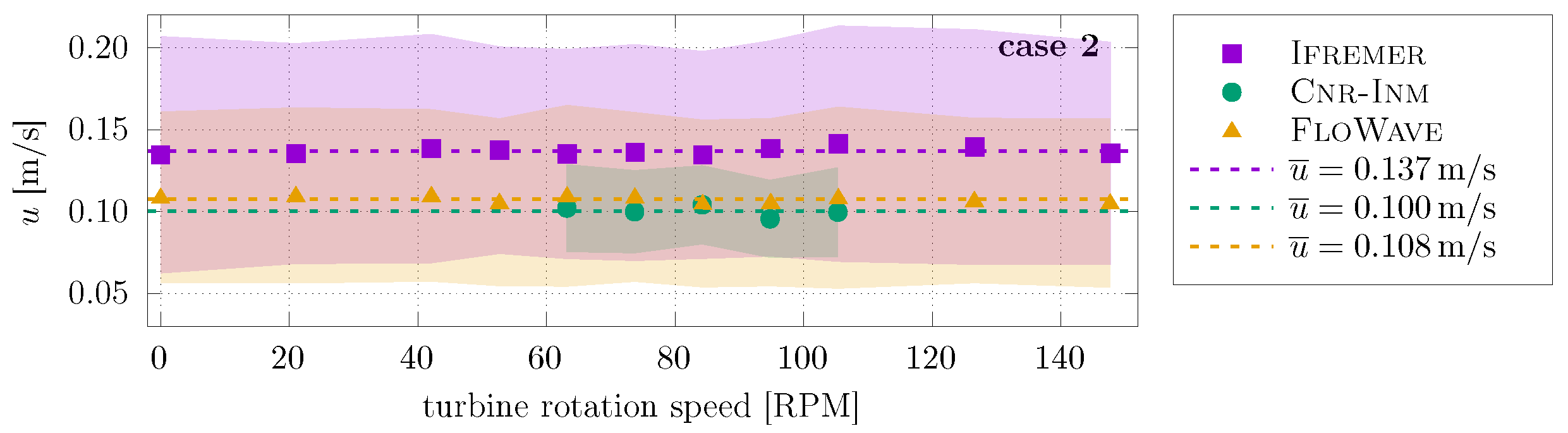
Figure 10.
Variation of the time-averaged (markers) and standard deviation (shading) of the horizontal wave orbital velocity u with rotational speed for case 2 at all facilities, obtained with the ADV. Dashed lines are the average of horizontal wave orbital for case 2 at all rotational speed settings per facility.
Figure 11.
Variation of the average (markers) and standard deviation (shading) of the wave amplitude
with rotational speed for case 2 at all facilities. Dashed lines are the average of the wave amplitude for case 2 at all rotational speed settings per facility. The red line indicates the target wave amplitude of case 2, data obtained with wave probe 3 (see
Figure 3).
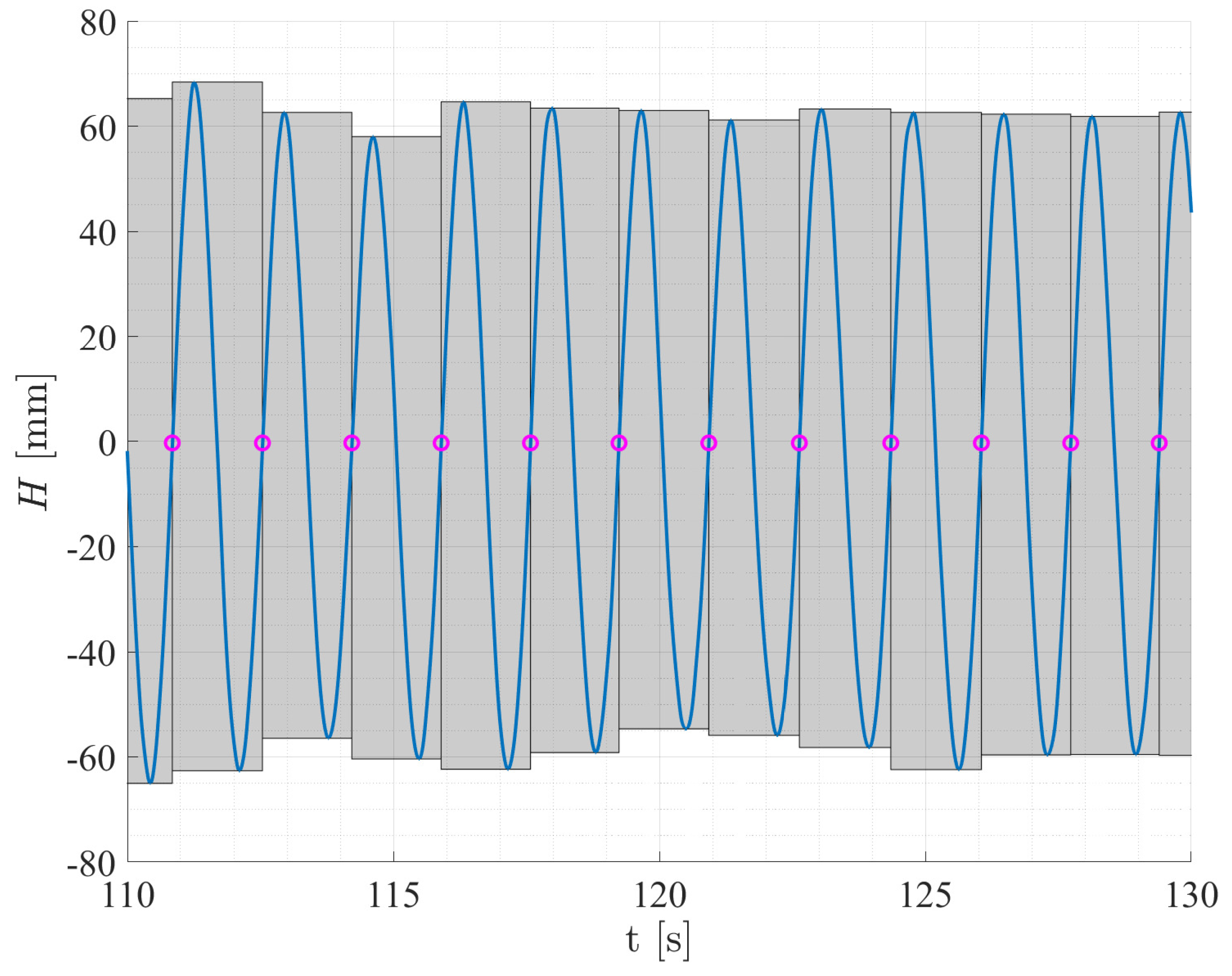
Figure 12.
Visual representation of the zero-up crossing method. Pink circles represent every time the signal crosses zero from negative to positive. The width of the greyed areas indicates the wave period and the height indicates the wave height.
Figure 12.
Visual representation of the zero-up crossing method. Pink circles represent every time the signal crosses zero from negative to positive. The width of the greyed areas indicates the wave period and the height indicates the wave height.
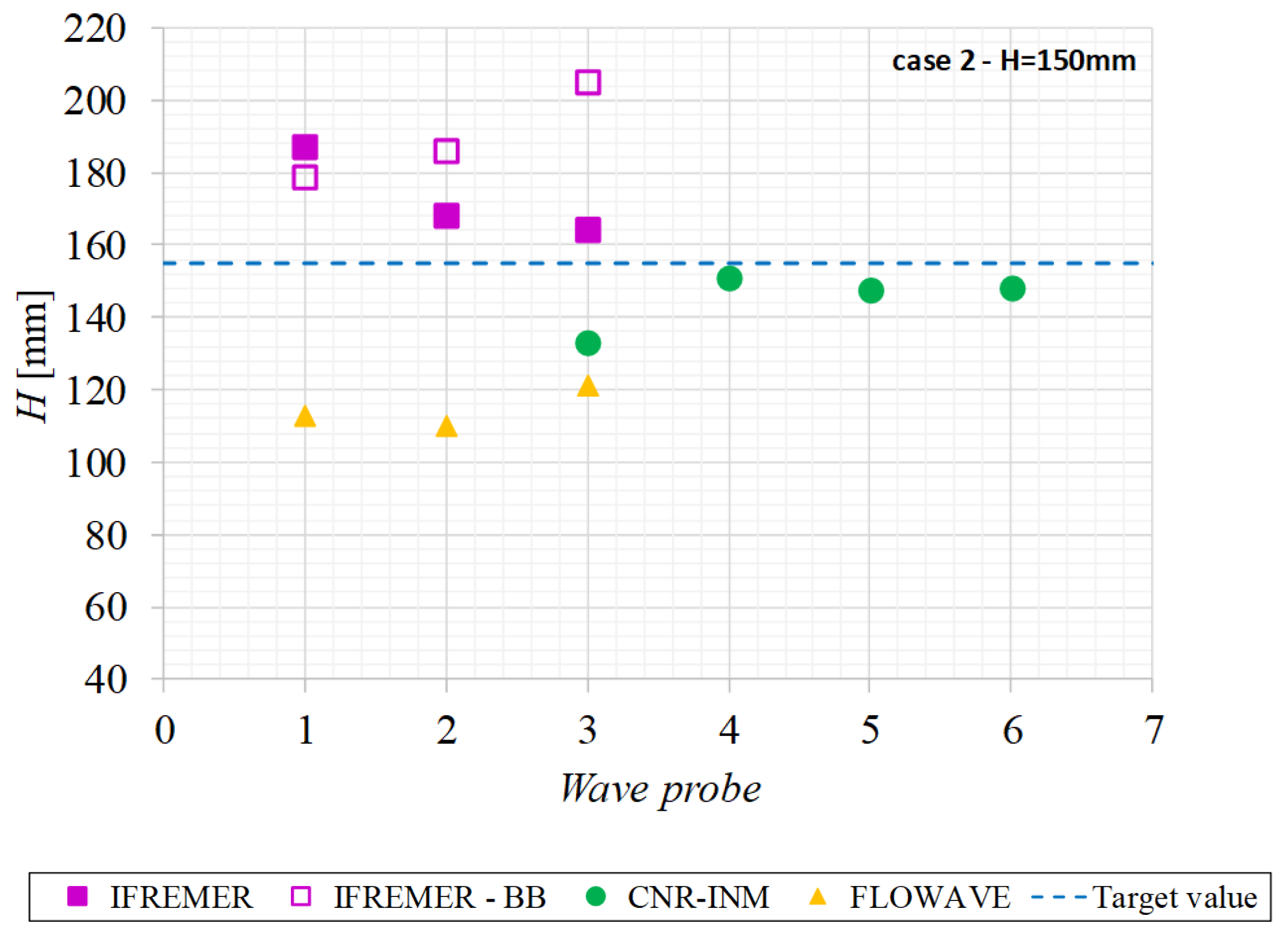
Figure 13.
Wave height
H comparison between the different wave probes at each facility for case 2.
Ifremer-BB are the bare-basin, flow characterisation tests. Dashed line represents the target wave height for case 2 of
. For the physical location of each wave probe, refer to
Figure 3.
Figure 13.
Wave height
H comparison between the different wave probes at each facility for case 2.
Ifremer-BB are the bare-basin, flow characterisation tests. Dashed line represents the target wave height for case 2 of
. For the physical location of each wave probe, refer to
Figure 3.
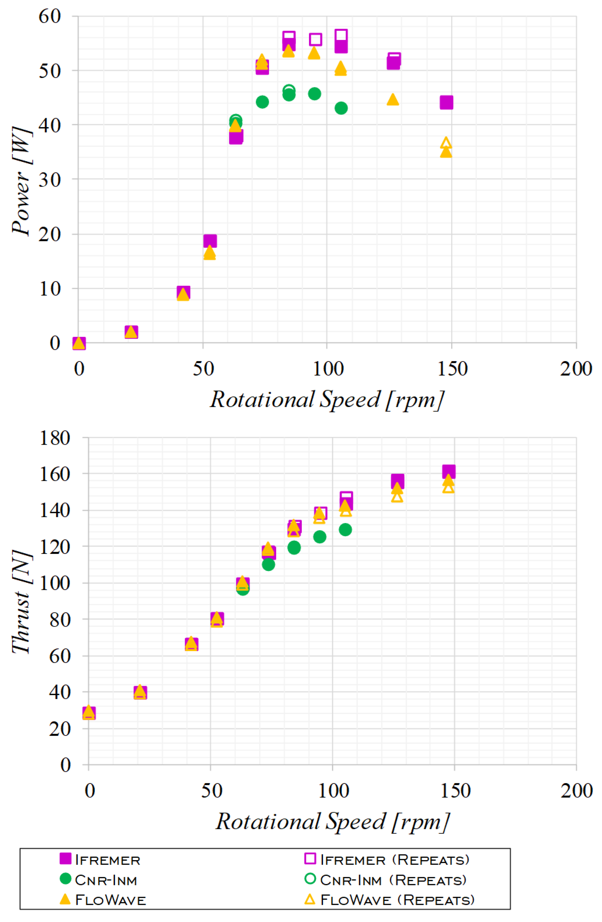
Figure 14.
Case 1: Variation of the time average of the power (top) and thrust (bottom) measurements against turbine rotational speed for cases at 0.8 m/s, taken at each of the facilities with the repeated tests when available.
Figure 14.
Case 1: Variation of the time average of the power (top) and thrust (bottom) measurements against turbine rotational speed for cases at 0.8 m/s, taken at each of the facilities with the repeated tests when available.
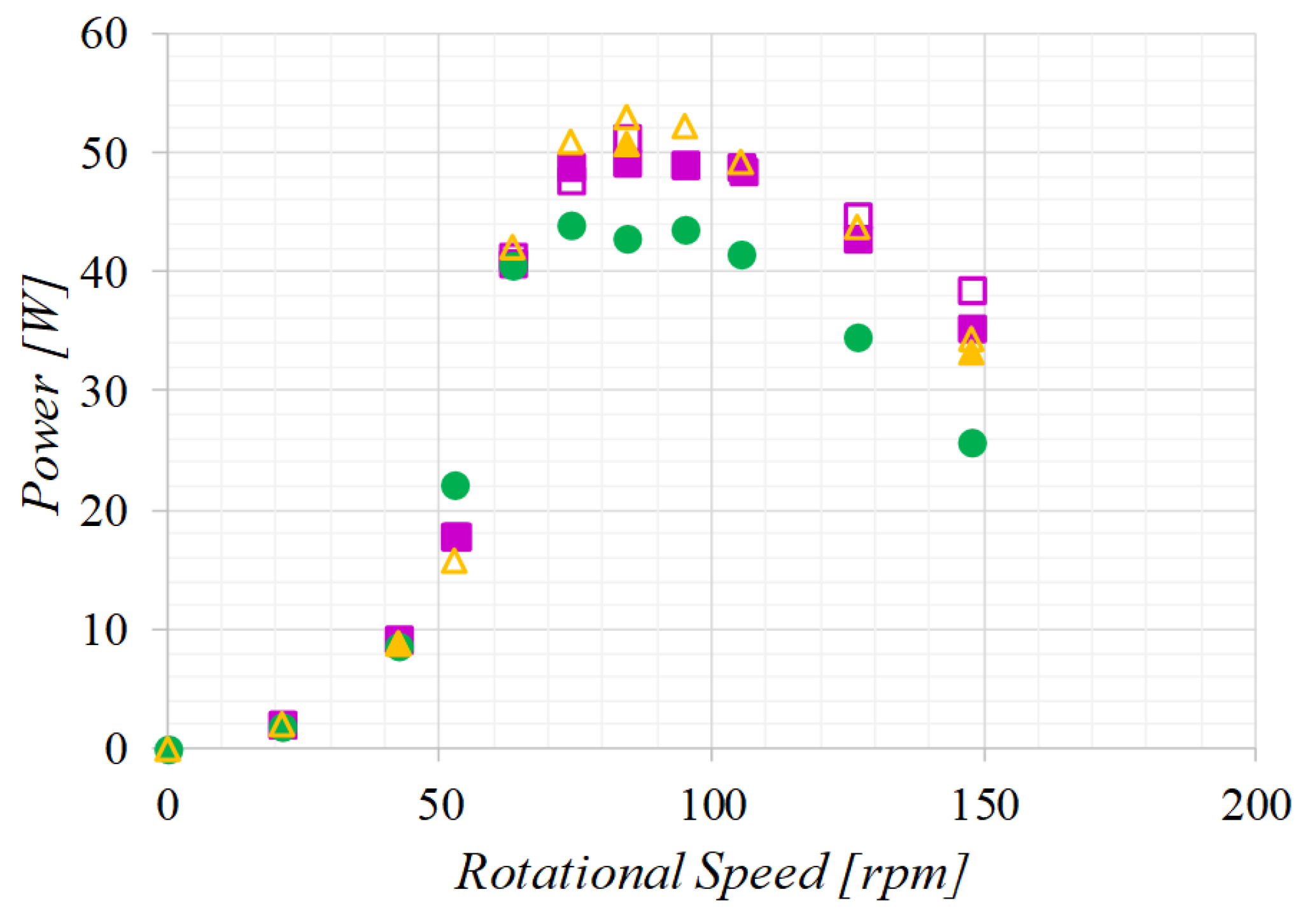
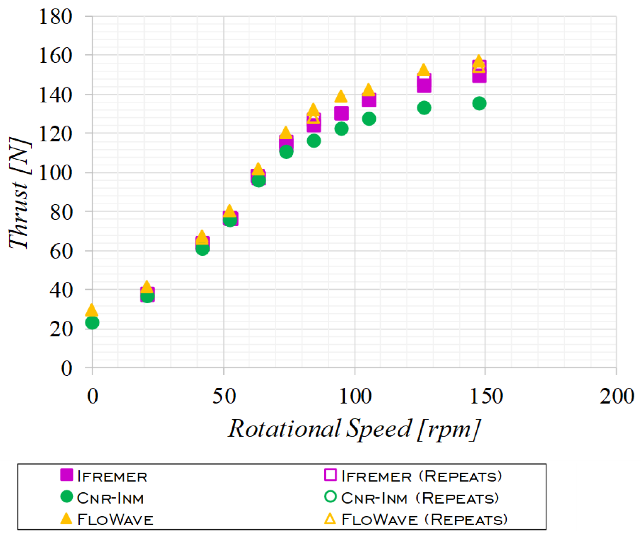
Figure 15.
Case 2: Variation of the time average of the power (top) and thrust (bottom) measurements against turbine rotational speed for cases at 0.8 m/s, taken at each of the facilities with the repeated tests when available.
Figure 15.
Case 2: Variation of the time average of the power (top) and thrust (bottom) measurements against turbine rotational speed for cases at 0.8 m/s, taken at each of the facilities with the repeated tests when available.
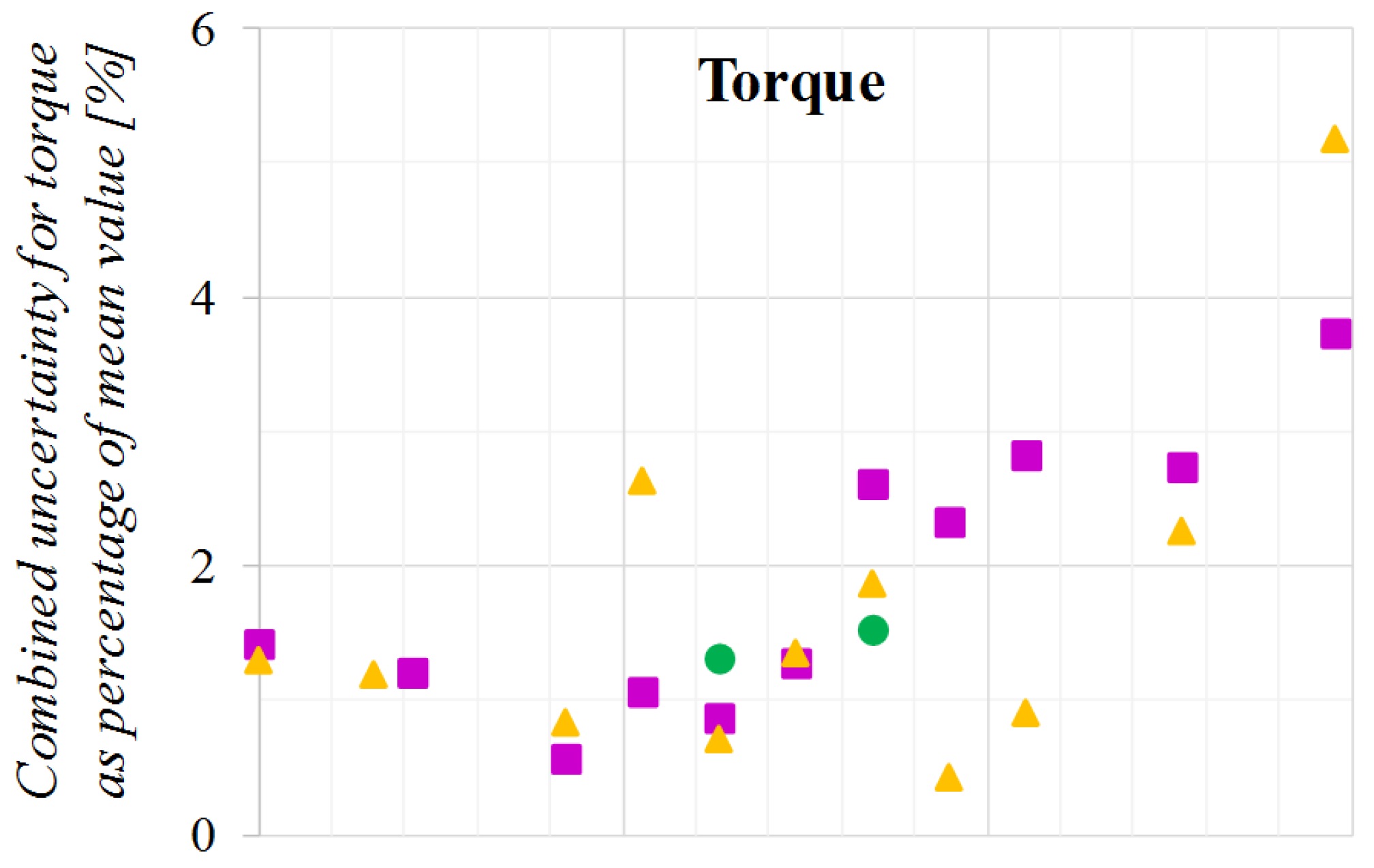
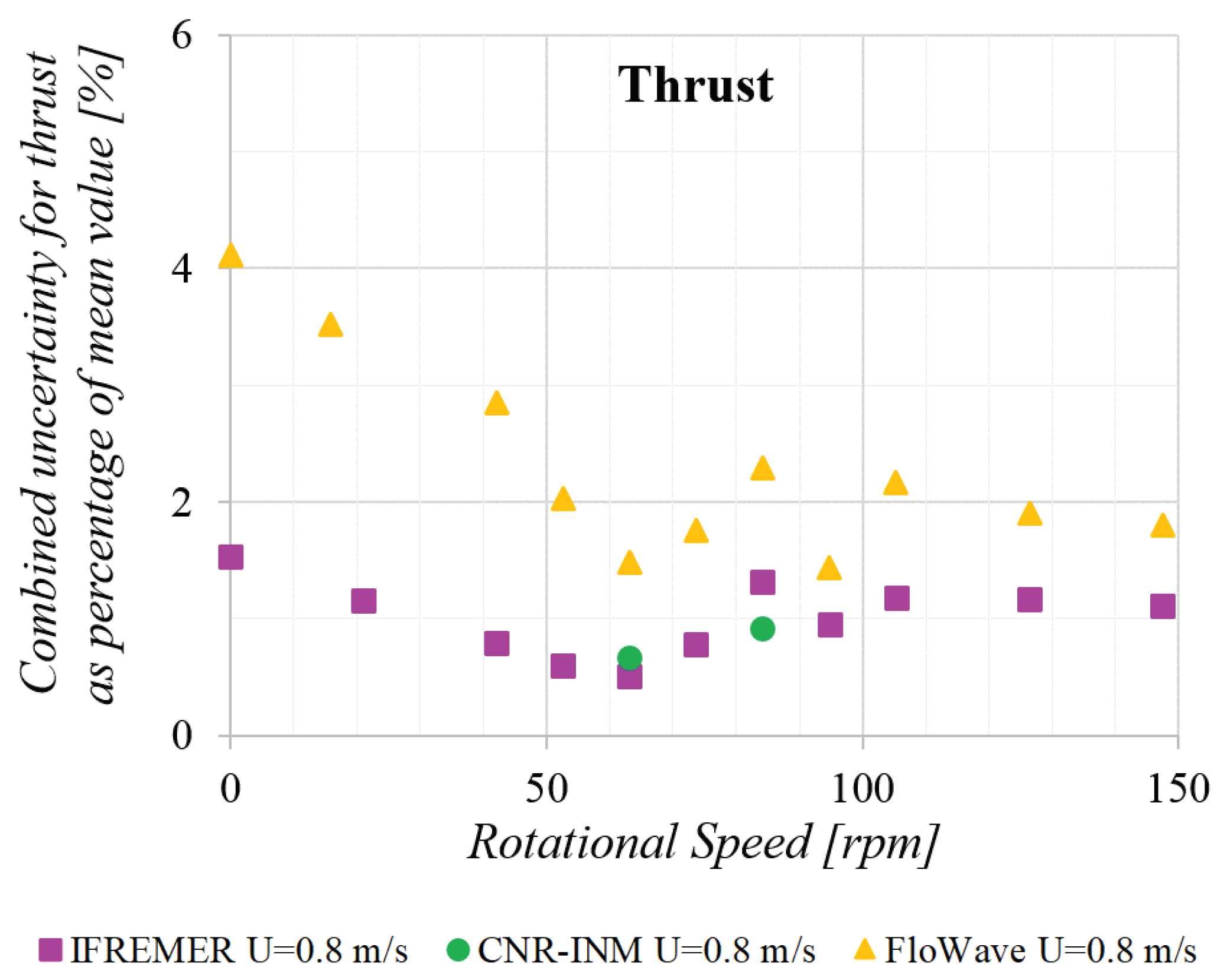
Figure 16.
Combined uncertainty for all cases at (i.e., cases 1, 2, 3 and 7) for torque (top) and thrust (bottom) as percentage of mean value based on the rotational speed for each the facilities.
Figure 16.
Combined uncertainty for all cases at (i.e., cases 1, 2, 3 and 7) for torque (top) and thrust (bottom) as percentage of mean value based on the rotational speed for each the facilities.
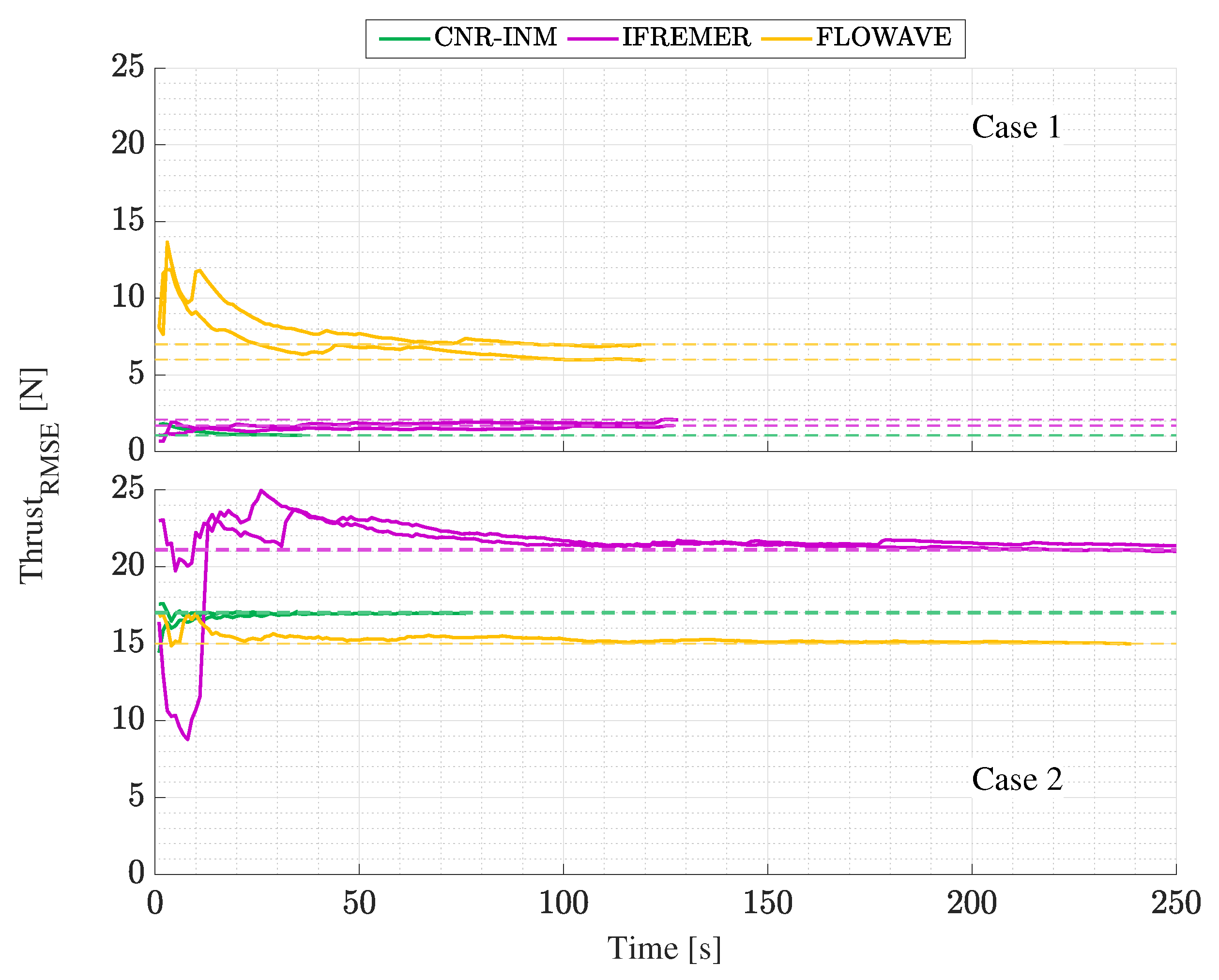
Figure 17.
Stabilisation of the thrust RMSE at for case 1 (top) and 2 (bottom) at all facilities. Dashed lines are the RMSE value of the whole time series; same-colour curves are repeat tests when available.
Figure 17.
Stabilisation of the thrust RMSE at for case 1 (top) and 2 (bottom) at all facilities. Dashed lines are the RMSE value of the whole time series; same-colour curves are repeat tests when available.
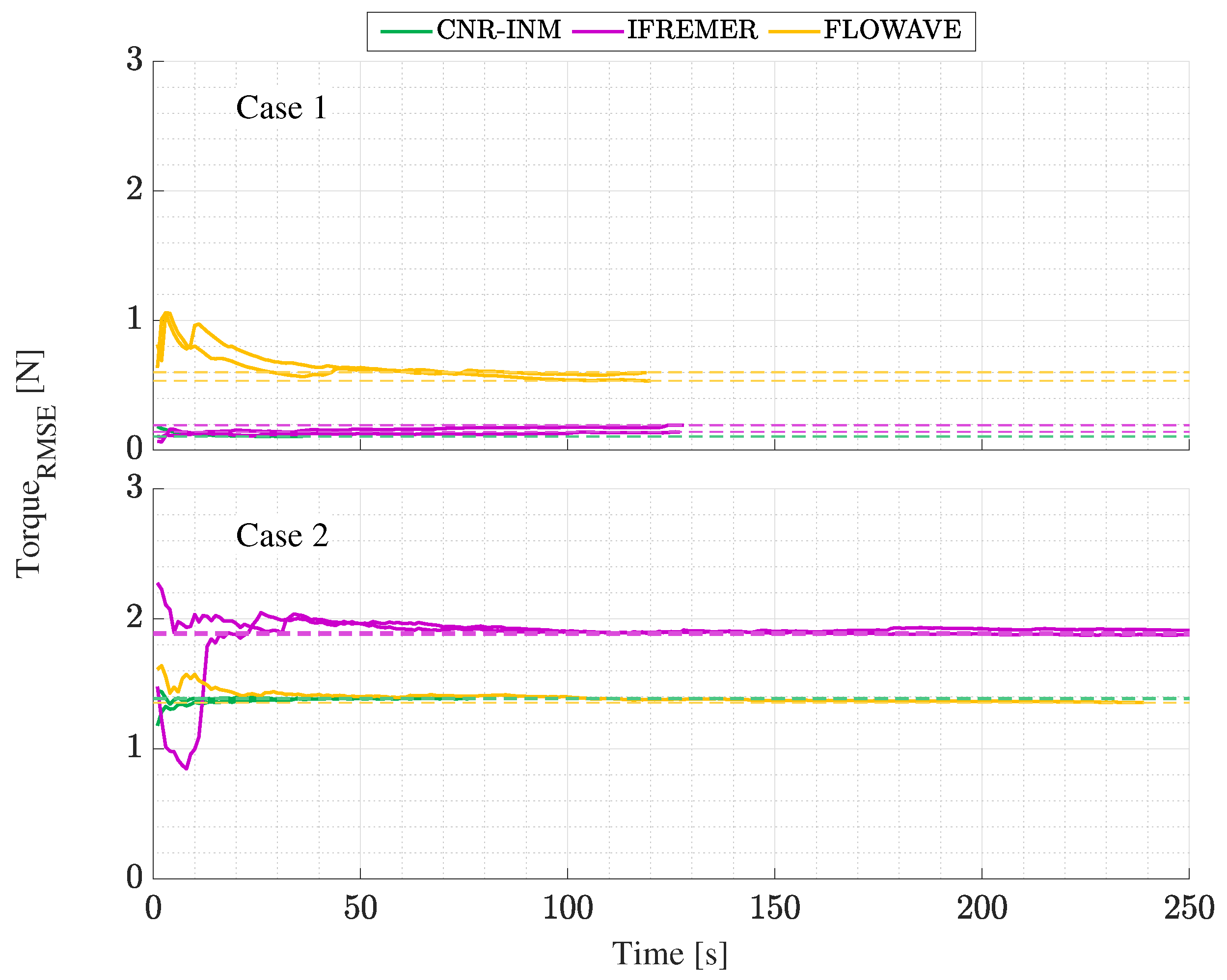
Figure 18.
Stabilisation of the torque RMSE at for case 1 (top) and 2 (bottom) at all facilities. Dashed lines are the RMSE value of the whole time series; same-colour curves are repeat tests when available.
Figure 18.
Stabilisation of the torque RMSE at for case 1 (top) and 2 (bottom) at all facilities. Dashed lines are the RMSE value of the whole time series; same-colour curves are repeat tests when available.
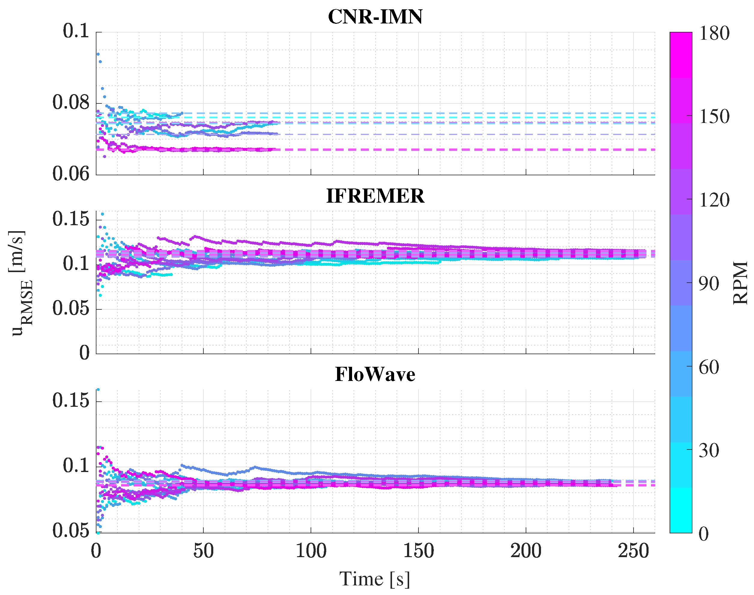
Figure 19.
Stabilisation of the RMSE of u for case 1 at all facilities.
Figure 19.
Stabilisation of the RMSE of u for case 1 at all facilities.
Table 1.
Wave–current interaction experiments undertaken with three-bladed HATTs.
Table 1.
Wave–current interaction experiments undertaken with three-bladed HATTs.
| Author | Facility | Rotor ∅ [m] | Wave Characteristics |
|---|
| Barltrop et al., 2007 [5] | Towing tank. Strathclyde University | 0.4 | Collinear regular waves |
| Gaurier et al., 2013 [6] | Flume tank. Ifremer | 0.9 | Collinear regular waves |
| Galloway et al., 2014 [7] | Towing tank. Southampton University | 0.8 | Collinear regular waves |
| Henriques et al., 2015 [8] | Flume tank. University of Liverpool | 0.5 | Collinear regular waves |
| Martinez et al., 2018 [9] | Flume tank. FloWave | 1.2 | Multi-directional regular waves |
| Ordonez-Sanchez et al., 2019 [10] | Towing tank. Cnr-Inm | 0.9 | Collinear regular and irregular waves |
| Draycott et al., 2019 [11] | Flume tank. FloWave | 1.2 | Collinear and opposing irregular waves |
| Draycott et al., 2019 [12] | Flume tank. FloWave | 1.2 | Focused wave groups |
| Porter et al., 2019 [13] | Flume tank. Ifremer | 0.9 | Collinear regular waves. Passively adaptive composite blades |
| Martinez et al., 2020 [14] | Flume tank. Ifremer | 0.9 | Collinear regular and irregular waves |
Table 2.
Main characteristics of the controlled testing facilities.
Table 2.
Main characteristics of the controlled testing facilities.
| Laboratory | Ifremer | Cnr-Inm | FloWave |
|---|
| Type of tank | flume | towing | flume |
| Length [m] | 18 | 220 | 10 |
| Width × Depth [m] | 4 × 2 | 9 × 3.5 | 10 × 2 |
| Speed range [m/s] | 0.1 to 2.2 | 0.1 to 10 | 0.1 to 1.6 |
| Turbulence int. [%] | 1.5 to 15 | - | 5 to 11 |
Table 3.
Measuring range and accuracy of turbine instrumentation.
Table 3.
Measuring range and accuracy of turbine instrumentation.
| Measured Signal | Operating Range | Accuracy |
|---|
| Thrust | | 0.2% |
| Torque | | 0.2% |
Table 4.
Summary of the test matrix.
Table 4.
Summary of the test matrix.
| Case | Type | Flow Speed [m/s] | Wave Frequency | Wave Amplitude [Hz] | Facilities Tested at [mm] |
|---|
| 1 | current | 0.8 | | | ifr, cnr, flw |
| 2 | regular | 0.8 | 0.6 | 75 | ifr, cnr, flw |
| 3 | regular | 0.8 | 0.5 | 35 | ifr, cnr, flw |
| 4 | current | 1.0 | | | ifr, cnr, flw |
| 5 | regular | 1.0 | 0.7 | 75 | ifr, cnr |
| 6 | regular | 1.0 | 0.6 | 55 | ifr, cnr, flw |
| 7 | irregular | 0.8 | 0.6 # | 100 * | ifr, cnr, flw |
Table 5.
Disc-integrated velocity average (DIVA) values for the flow characterisation without turbine for all cases at all facilities. See
Section 2.5.1, from [
15].
Table 5.
Disc-integrated velocity average (DIVA) values for the flow characterisation without turbine for all cases at all facilities. See
Section 2.5.1, from [
15].
| Case | Ifremer | Cnr-Inm | FloWave |
|---|
| 1 | 0.826 | 0.843 | 0.825 |
| 2 | 0.848 | 0.848 | 0.827 |
| 3 | 0.846 | N/A | 0.822 |
| 4 | 1.024 | 1.037 | 1.036 |
| 5 | 1.056 | 1.036 | N/A |
| 6 | 1.047 | N/A | 1.031 |
| 7 | 0.840 | N/A | 0.826 |
Table 6.
Time and case average of the ADV stream-wise velocity
u for all cases at all facilities. ADV mounted at
and
as seen in
Figure 3.
Table 6.
Time and case average of the ADV stream-wise velocity
u for all cases at all facilities. ADV mounted at
and
as seen in
Figure 3.
| Case Number | Ifremer | Cnr-Inm | FloWave |
|---|
|
|---|
| 1 | 0.840 | 0.824 | 0.885 |
| 2 | 0.886 | 0.832 | 0.892 |
| 3 | 0.869 | 0.840 | 0.886 |
| 4 | 1.050 | 1.025 | 1.105 |
| 5 | 1.094 | 1.042 | - |
| 6 | 1.084 | 1.039 | 1.103 |
| 7 | 0.876 | 0.899 | 0.890 |
Table 7.
Time-average of the horizontal wave orbitals u measured by the ADV at the turbine hub height for all cases at all facilities.
Table 7.
Time-average of the horizontal wave orbitals u measured by the ADV at the turbine hub height for all cases at all facilities.
| Case Number | Ifremer | Cnr-Inm | FloWave |
|---|
|
|---|
| 2 | 0.137 | 0.100 | 0.108 |
| 3 | 0.119 | 0.056 | 0.086 |
| 5 | 0.136 | 0.094 | - |
| 6 | 0.139 | 0.082 | 0.102 |
| 7 | 0.088 | 0.038 | 0.087 |
Table 8.
Time and case average of the wave amplitude
for all cases at all facilities. Data obtained from wave probe 3 (see
Figure 3) in synchronisation with the turbine.
Table 8.
Time and case average of the wave amplitude
for all cases at all facilities. Data obtained from wave probe 3 (see
Figure 3) in synchronisation with the turbine.
| Case Number | Target | Ifremer | Cnr-Inm | FloWave |
|---|
|
|---|
| 2 | 75 | 87 | 66 | 60 |
| 3 | 35 | 37 | 30 | 26 |
| 5 | 75 | 72 | 62 | - |
| 6 | 55 | 61 | 50 | 26 |
| 7 | 100 * | 40 | 35 | 35 |
Table 9.
Comparison of the combined expanded uncertainty as a percentage of the average value based on Equations (
1) and (
2).
Table 9.
Comparison of the combined expanded uncertainty as a percentage of the average value based on Equations (
1) and (
2).
| Facility | Torque [%] | Thrust [%] | Rotational Speed [%] |
|---|
| Cnr-Inm | 1.48 | 0.68 | 0.04 |
| FloWave | 4.21 | 3.13 | 0.07 |
| Ifremer | 1.60 | 0.91 | 0.11 |
Table 10.
Combined uncertainty for torque as percentage of mean value based on the case number for each facility [%]. Current-only cases at Cnr-Inm have no repeats.
Table 10.
Combined uncertainty for torque as percentage of mean value based on the case number for each facility [%]. Current-only cases at Cnr-Inm have no repeats.
| Case | Facility |
|---|
| Cnr-Inm | FloWave | Ifremer |
|---|
| 1 | - | 2.81 | 2.52 |
| 2 | 1.45 | 1.44 | 1.31 |
| 3 | 1.37 | 1.53 | 1.71 |
| 4 | - | 15.28 | 1.93 |
| 5 | 0.72 | - | 1.12 |
| 6 | 0.78 | 1.90 | 1.30 |
| 7 | - | 2.24 | 1.89 |
Table 11.
Combined uncertainty for thrust as percentage of mean value based on the case number for each facility [%]. Current-only cases at Cnr-Inm have no repeats.
Table 11.
Combined uncertainty for thrust as percentage of mean value based on the case number for each facility [%]. Current-only cases at Cnr-Inm have no repeats.
| Case | Facility |
|---|
| Cnr-Inm | FloWave | Ifremer |
|---|
| 1 | - | 2.35 | 1.37 |
| 2 | 0.76 | 2.84 | 0.98 |
| 3 | 0.81 | 3.68 | 1.01 |
| 4 | - | 7.74 | 0.88 |
| 5 | 0.59 | - | 0.90 |
| 6 | 0.54 | 1.15 | 1.00 |
| 7 | - | 0.96 | 0.98 |


 ,
, 


