Topological and Morphological Controls on Morphodynamics of Salt Marsh Interiors

Abstract

Salt marshes are important coastal environments and provide multiple benefits to society. They are considered to be declining in extent globally, including on the UK east coast. The dynamics and characteristics of interior parts of salt marsh systems are spatially variable and can fundamentally affect biotic distributions and the way in which the landscape delivers ecosystem services. It is therefore important to understand, and be able to predict, how these landscape configurations may evolve over time and where the greatest dynamism will occur. This study estimates morphodynamic changes in salt marsh areas for a regional domain over a multi-decadal timescale. We demonstrate at a landscape scale that relationships exist between the topology and morphology of a salt marsh and changes in its condition over time. We present an inherently scalable satellite-derived measure of change in marsh platform integrity that allows the monitoring of changes in marsh condition. We then demonstrate that easily derived geospatial and morphometric parameters can be used to determine the probability of marsh degradation. We draw comparisons with previous work conducted on the east coast of the USA, finding differences in marsh responses according to their position within the wider coastal system between the two regions, but relatively consistent in relation to the within-marsh situation. We describe the sub-pixel-scale marsh morphometry using a morphological segmentation algorithm applied to 25 cm-resolution maps of vegetated marsh surface. We also find strong relationships between morphometric indices and change in marsh platform integrity which allow for the inference of past dynamism but also suggest that current morphology may be predictive of future change. We thus provide insight into the factors governing marsh degradation that will assist the anticipation of adverse changes to the attributes and functions of these critical coastal environments and inform ongoing ecogeomorphic modelling developments.

1. Introduction

Salt marshes represent a major component of low-lying sedimentary coastal systems and occur across the world [1]. Over recent decades, salt marshes have attracted increasing attention, with much research being focused on the services and functions they provide [2]. Salt marshes exhibit an extremely high biodiversity [3] and primary productivity [4]. They attenuate wave energy and contribute significantly to the protection provided by natural foreshores from high waves and water levels threatening coastal communities [5,6]. Marshes are a sink for atmospheric carbon [7,8,9], while providing a habitat for many endangered or threatened species and nursery areas for commercial fish stock species [10,11]. They also have cultural value as areas for recreation and tourism. In the UK, over the last 150 years map and aerial imagery suggest an expansion of marsh areas in northern England, as against areal loss in the south, attributed to regional variations in sediment supply [12]. It has, however, proven difficult to ascertain patterns of marsh areal change and controlling factors over the latter half of the twentieth century. The East Anglian coast (Figure 1) is thought to be a region with high rates of wetland loss (e.g., [13]), but in reality rates and types of marsh loss have exhibited great spatial variability (e.g., [14]). Furthermore, achieving precise estimates of changes in marsh area has been shown to be challenging by the few large-scale UK inventories attempted [15,16,17].

The position of a marsh system within a broader context of the coastal zone exerts controls on factors such as sediment or nutrient import and export, tidal flushing and residence times, and forces exerted by tidal currents. The connectivity between intertidal wetland areas and offshore deep channel zones is crucial to water, sediment, and nutrient exchange and thus to the morphological evolution of marshes [18].

The position of a marsh parcel within the surrounding system, and the position of a point on the marsh within individual parcels, modulate local-scale responses. There has long been recognition that elevation–sedimentation relationships vary with scale. For example, single-tide sediment deposition decreases with distance from tidal channels, while surface elevation provides an important marsh-wide control over annual to decadal timescales [19]. Kearney and Rogers [20] previously used logistic regression to predict internal platform integrity changes in marshes at a regional scale in Chesapeake and Delaware Bays, USA. They demonstrated empirical relationships between changes in marsh surface condition and factors such as distance up-estuary and position within a marsh parcel. The marsh systems on the UK East coast have a different context (tidal range, position within tidal frame, sedimentology, vegetation community) to those studied by Kearney and Rogers [20] but we are able to draw comparisons between the topological relationships presented here and their findings.

The morphology of the marsh, described by the spatial distribution of landscape units (at a scale of metres) such as vegetated platforms, salt pans, creeks, and large channels, is the integrative result of historic morphodynamics [21]. Morphology is also thought to exert a control on future changes through biogeomorphic feedback [22], while the interactions between topography and hydrodynamic forces have been extensively explored from a numerical perspective [23]. From an empirical perspective, a relationship between the functional form of marsh margins and erosion rates has been demonstrated [24].

Of particular, and most immediate, interest for landscape management are the loci of greatest dynamism; the most important to understand when considering future ecosystem service provision are those exhibiting (or likely to exhibit) erosion. This study aims to assess the decadal morphodynamics of salt marsh systems on the east coast of the UK, evaluate the role of topological and morphological factors in determining the observed changes, and provide understanding of the controls on salt marsh morphological evolution to support ecosystem management and the development of models that combine ecological and physical functioning. We present landscape-scale statistical models relating such changes to easily derived spatial parameters at scales from the regional (tens of kilometres) to local (metres). Such understanding will help with the prediction of locations likely to exhibit degradation accompanied by concomitant losses of ecosystem services. This will thereby facilitate targeted management interventions to protect the ecological and physical functioning of these important coastal ecosystems.

2. Materials and Methods

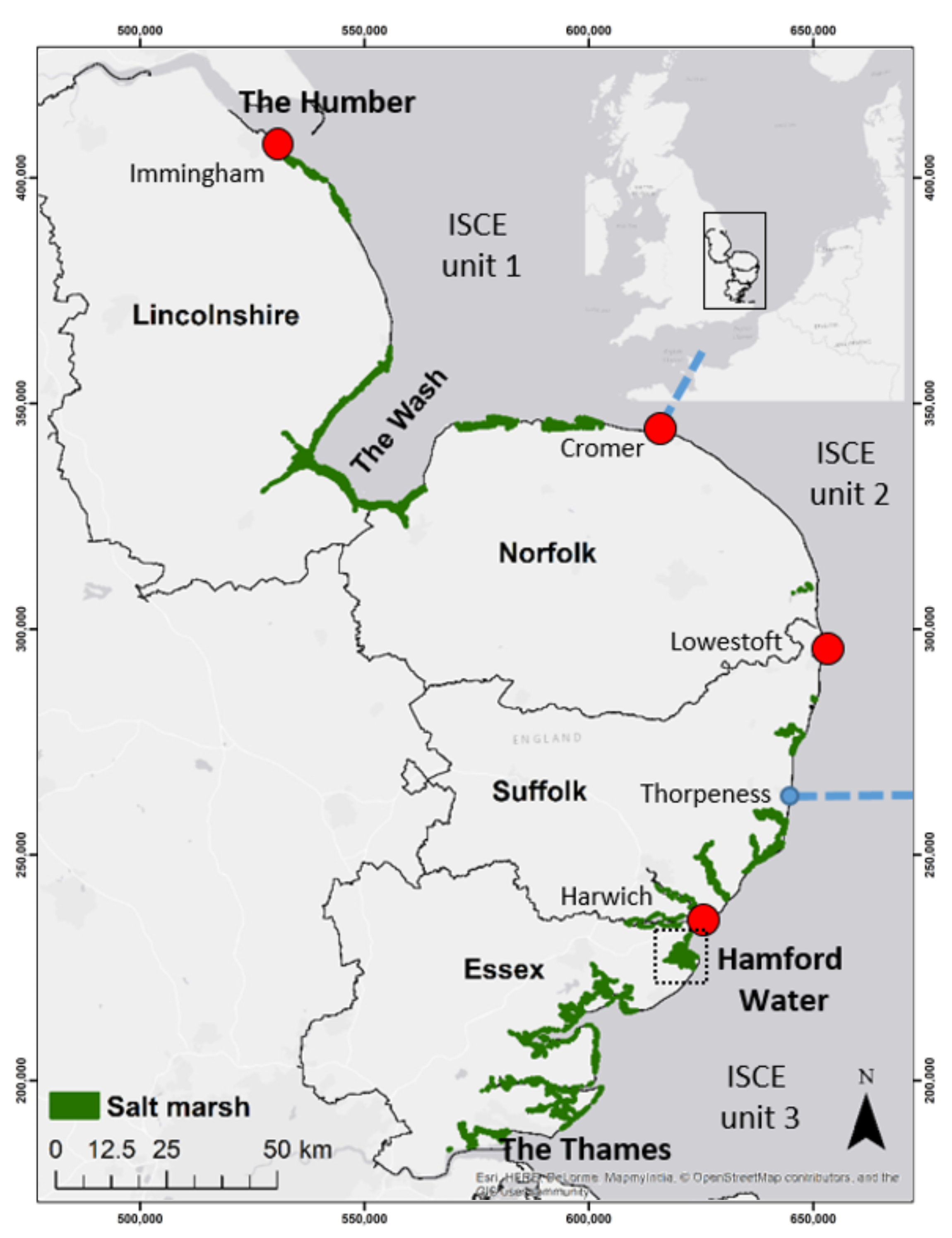
2.1. Study Area

The coastline of East Anglia, UK, is bounded by the Humber estuary to the north and the Thames estuary to the south (Figure 1). The region is, in many parts, densely populated. The population in the coastal districts of Suffolk and Norfolk exceeds 600,000 (Office for National Statistics GB 2016 census data—www.ons.gov.uk/census accessed on 23 October 2018). A considerable amount of variability occurs along this stretch of coast in terms of the hydrodynamic and sedimentary contexts. The mean spring tidal range (MSTR) varies from 6.18 m at Immingham on the Humber to a minimum of 1.94 m at Lowestoft, Suffolk, before increasing again further south (ntslf.org accessed on 10 December 2020).

Pethick and Leggett [25] partitioned the region into three Integrated Scale Coastal Evolution (ISCE) units. The Northern ISCE includes the eroding glacial cliffs north of the Humber, which provide sediment inputs for the sandy shorelines in Lincolnshire and the infilling embayment of The Wash. The ISCE includes the spit and barrier island system of the north Norfolk coast as far east as Cromer. The second ISCE is dominated by cliffs composed of glacial sands and gravels and lies between Cromer and Thorpeness. The third, southerly, unit comprises numerous estuaries and inlets sitting within a large embayment and characterised by silt or clay sediments [26]. The region contains some 14,406 ha of salt marsh [17] of diverse character and setting; open coast, embayment, back-barrier, and estuarine marshes are represented [27]. Suffolk and Essex have both experienced a net loss of marsh area in the second half of the twentieth century [15] while The Wash embayment, between Norfolk and Lincolnshire, represents a long-term sediment sink [28] and continues to infill [26], with attendant increases in marsh area [24]. At the regional scale, none of these systems can be thought of as ’sediment starved’.

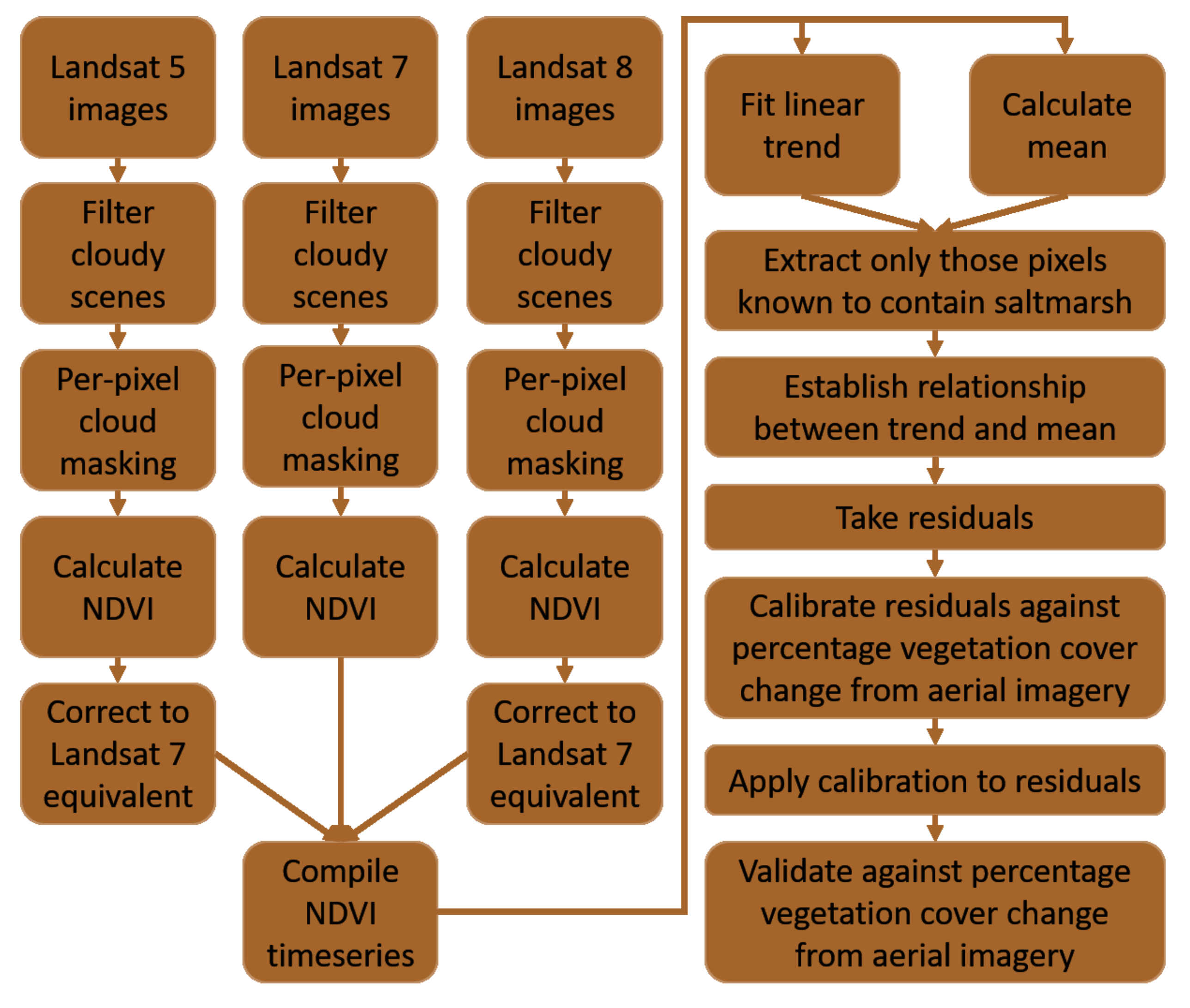
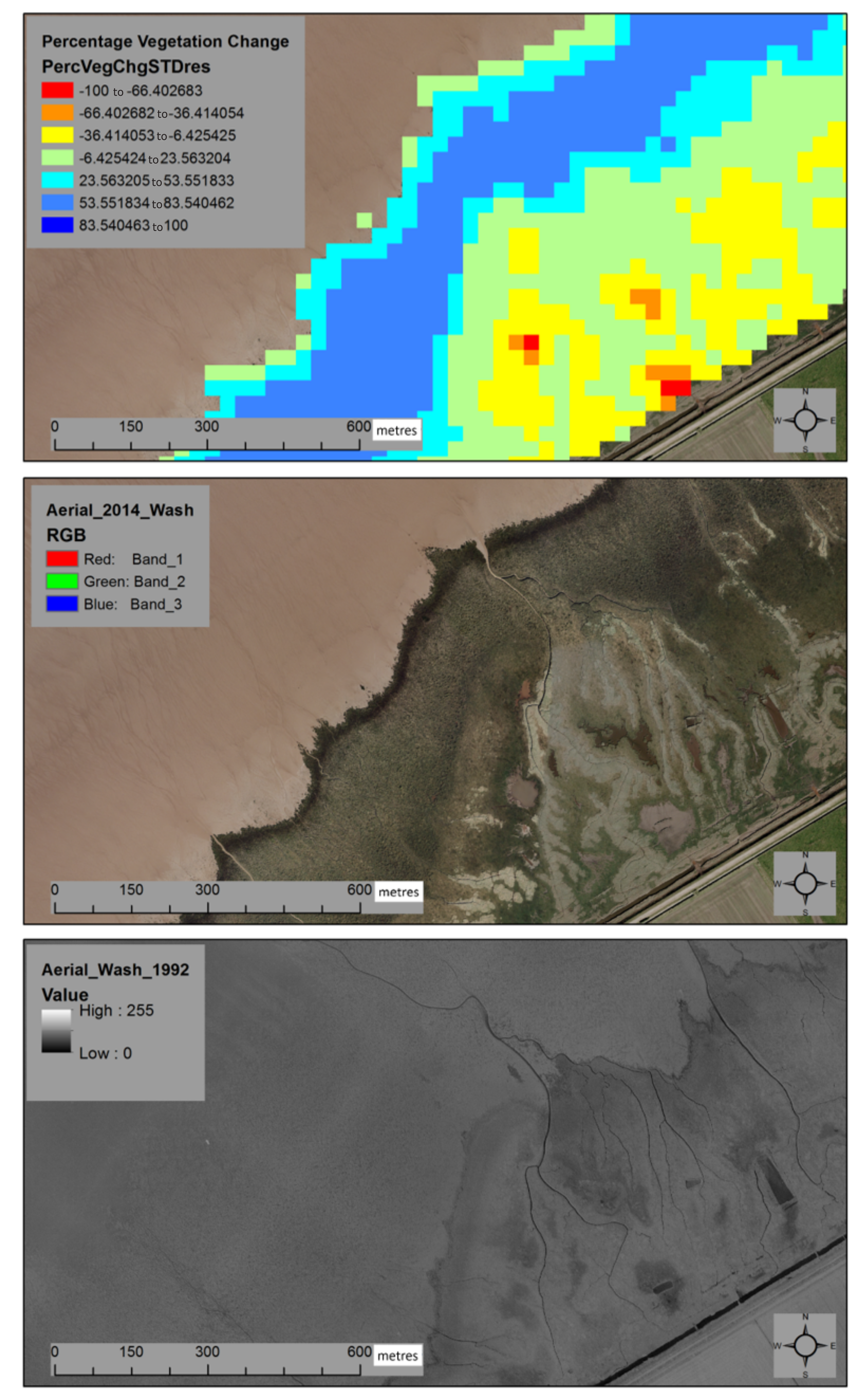
2.2. Morphological Change

We address controls on morphodynamic change within marsh interiors comprising the complex morphologies of vegetated surfaces, creeks, pools, and pans that lie landward of the seaward margin of the marsh as a whole. We use satellite imagery to estimate changes in vegetation distributions within these areas, from which we infer morphological changes. This inference is based on well-established elevational controls on intertidal vegetation establishment [29], which have been thoroughly ground-referenced for NW Europe by Suchrow and Jensen [30]. In inferring morphological change, we assume that all surfaces of sufficient elevation to support vegetation become colonised, while those that are too low do not.

Changes in the extent of vegetation within marsh interiors were estimated using a modified trend analysis of the Landsat archive, which represents the longest appropriate satellite time series available (1984–present). Imagery dating between 1985 and 2016 was used in this study. The exact time period over which the metric is calculated will vary slightly between pixels due to the different acquisition dates of imagery over certain areas and cloud cover precluding the use of some pixels (see https://osf.io/mgsyz/).

A metric was derived, denoted $\delta P_{veg}$, that can be interpreted as representing the percentage change in vegetation cover within any given pixel over the timeframe of the satellite observations. As such, it reflects the temporal variations in the areal unvegetated–vegetated marsh ratio (UVVR) within each 30 m by 30 m pixel. The UVVR could be considered a geomorphic metric that has itself been shown to be related to marsh vulnerability [31]. The methodological workflow we use is summarised in Figure 2 and is detailed extensively in Appendix A.

In Google Earth Engine [32], the Normalised Difference Vegetation Index (NDVI), a proxy for the amount of chlorophyll (and therefore vegetation) present, was computed for all scenes within the Landsat archive for the study region up to 2016. Conceptually, the NDVI for a pixel in a satellite image can be considered to be a function of the percentage of that pixel covered by vegetation and the nature of the vegetation within that pixel. A change in the NDVI reflects a change in the percentage vegetation cover within the pixel, with the signal potentially being modulated by any attendant changes in community composition (and therefore spectral signature) and the vigour of the vegetation present. Lopes et al. [33] evaluted a number of vegetation indices for the monitoring of salt marsh extent and condition in Portugal based on the Landsat archive and concluded that NDVI performed best, with a seasonally varying goodness-of-fit [34] typically exceeding 0.9 at one location and 0.75 at another, where a perfect classification would result in a value of 1.

NDVI values were cross-calibrated to account for differences in radiomemtric response between different Landsat sensors before a linear trend was computed over the time series for each pixel. A relationship between the coefficients of the trend and the mean NDVI over the time series was found, which was removed by taking the residuals of the regression fit between the slope of the trend line and the mean NDVI ($R^2=0.22$, $p\le 0.001$). The resulting residuals were standardised and calibrated against 25cm Environment Agency aerial photography from 1992 and 2013/14. Calibration was achieved by the visual assessment of the aerial photography subsets extracted for a random sample of satellite pixels (n = 83) stratified to represent the full range of observed standardised residual trend coefficents. For each satellite pixel area, 50 points were randomly distributed and each was manually classified as either coinciding with vegetated or unvegetated surfaces in both the 1992 and 2013/14 aerial photography. For each year, the percentage of satellite pixel area that was vegetated in the aerial photography was then calculated based on the counts in each surface cover class. A strong relationship was found between the satellite-derived residuals and the photography-based estimates of change in vegetation cover ($R^2=0.87$, $p\le 0.001$), implying that changes in vegetation extent dominate changes in $\delta P_{veg}$. The calibration sample was drawn from the entire study region. $\delta P_{veg}$ varies in the range −100% to +100%, where −100% represents a change from fully vegetated to fully bare and +100% the opposite. The method was validated against a sample of pixels representative of the full range of calibrated estimates (n = 100) but drawn from a local subset area (Hamford Water, Essex) to obviate the effect of any large-scale (e.g., latitudinal) signal that may have been present within the calibration. The $\delta P_{veg}$ metric performed well, with an RMSE of 11.9% of full scale (±100%).

2.3. Topological and Morphological Metrics

Two metrics were derived to describe the topology of a location within a marsh and two morphological metrics were developed to describe the distribution of landscape units within a single Landsat pixel area.

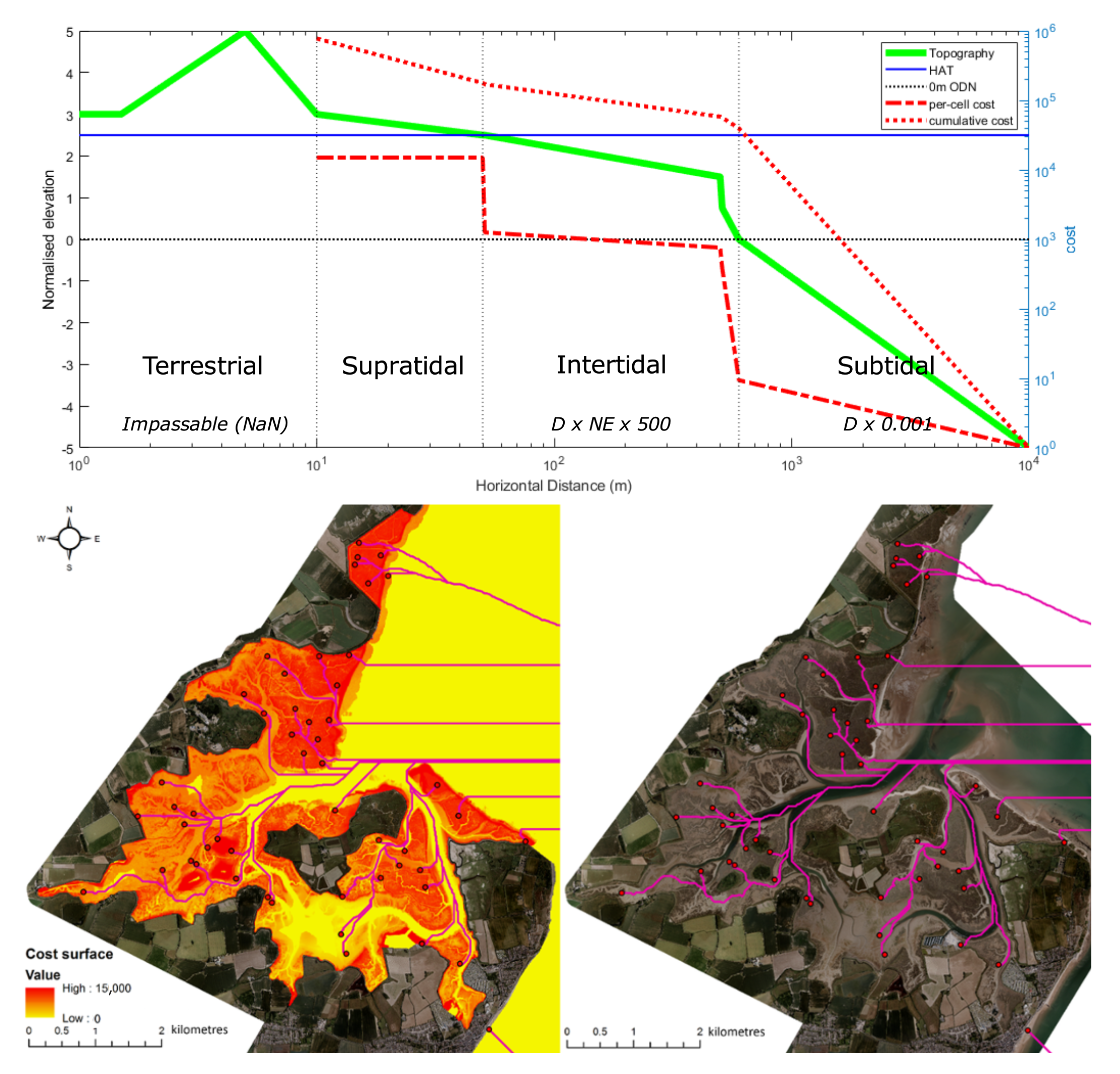
2.3.1. Geomorphic Setting

The geomorphic setting of the marsh, meaning its context within the wider coastal system, was represented as a cost function, denoted Cost Distance (CD), describing how difficult it would be for a parcel of water originating offshore to reach any given location within a marsh. Thus, for example, interior marsh areas towards the head of estuaries are more ’costly’ to reach (less well connected to the offshore) than the seaward margins of open coast marshes. Without a full simulation of tidal exchanges against which to calibrate flow pathways, the CD metric is not expected to behave in an isomorphic manner with actual tidal exchanges. Rather, CD values are internally consistent and represent a scale of relative connectivity within the study domain.

The area between the 10 km offshore limit and the land was represented on a 10 m grid and divided into four zones. For ease, we denote these ‘subtidal’, ‘intertidal’, ’supratidal’, and ’terrestrial’, while recognising that they do not conform strictly to these descriptions. Intertidal, for example, would ordinarily refer to elevations between the lowest and highest tides experienced. In the UK, this range would extend well below 0 m Ordnance Datum Newlyn (ODN), which approximates mean sea level but is used here as the lower bound of the ‘intertidal’ zone (see below). The landward limit was defined by the UK Environment Agency Second Generation Shoreline Management Plan as segments vector layer(SMP2), which typically reflects the line of engineered defences. Costs to traverse each cell of the grid were based on distances, with the cells in each zone given different weighting factors. Areas below 0 m ODN were denoted ’subtidal’ and were assigned a cost according to their euclidean distance in metres from the offshore boundary.

An ‘intertidal’ zone was defined as areas between 0 m ODN and the level of the highest astronomical tide (HAT). Elevations were derived from the Environment Agency 2 m-resolution LiDAR composite product (2008) resampled to the 10 m grid. Since spatially resolved data describing HAT were not available, modelled MSTR values [35] were extrapolated to intersect the shoreline and an $0.7\times$ MSTR was used to approximate the level of HAT. Our comparison of the levels thus estimated and known levels at the four standard ports in the study region (Immingham, Cromer, Lowestoft, and Felixstowe) suggests that this approximation tends to slightly overestimate (order of 10 cm) the level of HAT. The dependency of intertidal wetland development on tidal range is well documented, with equivalent landforms occurring at higher levels relative to the mean sea level in macrotidal settings than in microtidal ones [27,36]. The elevation range available for the development of intertidal landforms can be described as an ‘accommodation range’. The DEM elevations above 0 m ODN were therefore normalised to reflect the spatial variability in accommodation range, which was itself approximated as $0.5\times$ MSTR. This produced a normalised elevation (NE) raster that did not exhibit substantial dependency on tidal range and was used to scale the resulting cost functions for the intertidal zone.

A ‘supratidal’ zone was defined as areas above HAT but seaward of the SMP2 vector marking the terrestrial limit. Such areas may still be inundated and therefore permit water flow during exceptional events, so this zone was given a uniform but very high cell cost relative to the other zones. A ‘terrestrial’ zone landward of engineered defences was modelled as impassable for tidal waters.

The zones were combined to produce an overall cost surface raster which was converted to a cost-distance raster where each cell value represents the cumulative cost to reach it by the least-cost path from the 10 km offshore limit of the domain. The weightings for each zone were manually adjusted to produce the best achievable visual replication of expected flow routes for tidal waters to reach a given location through complex channel networks. Figure 3 shows a schematic cross-shore transect from the engineered defence to the 10 km offshore limit of the domain (top panel). Per-cell and cumulative costs are plotted in red, with the levels of 0 m ODN and HAT also indicated. The four zones upon which the overall cost surface was based are indicated along with their final weighting functions (where D is the horizontal distance in metres and NE is the normalised elevation). The lower panel of Figure 3 shows examples of the least-cost paths calculated for random pixels superimposed on both the local per-pixel cost surface and aerial photography to demonstrate the ability of the method to reproduce expected flow routes.

2.3.2. Distance from Creek/Edge of Marsh Parcel

This measure represents the well-established tendency for sediments to be deposited rapidly once creek banks become overtopped during inundation, leading to the development of creek levees and limited deposition rates in areas away from cliffed seaward margins [37,38]. To represent this dynamic, a measure of distance from a creek or the edge of a marsh parcel was used. To facilitate analysis at scales commensurate with the size of Landsat pixels used for other variables (30 m by 30 m), a reduced resolution product representing offshore or large-creek margins of marsh parcels was derived from the Environment Agency’s salt marsh extent layer [17]. Large creeks were defined as those wider than the diagonal of a Landsat pixel (ca. 42.5 m), since these are the units for which internal morphological changes were measured. Creeks and pools narrower than 42.5 m were removed using a 21.25 m outer buffer on the polygons of the salt marsh extents layer, followed by the dissolving of any overlaps thus created and 21.25 m inner buffer operations. This spatial resolution limit, imposed by the buffering process, effectively disregards the smaller creeks, which nevertheless perform important system functions. This fact must be taken into account when interpreting the findings, and we comment further on this aspect in the discussion. The other metrics used, including $\delta P_{veg}$, are not sensitive to spatial resolution limits in the same manner.

Landward limits of the marsh polygons were removed by extracting only those portions of perimeter lines that were greater than 30 m (1 landsat pixel) from the SMP2 vector, ensuring that distances do not represent those from the landward limit. For each parcel, the euclidean distance from the edge was then calculated on a 30 m grid aligned to that used for $\delta P_{veg}$ estimation. The metric is henceforth referred to as Euclidean Distance (ED).

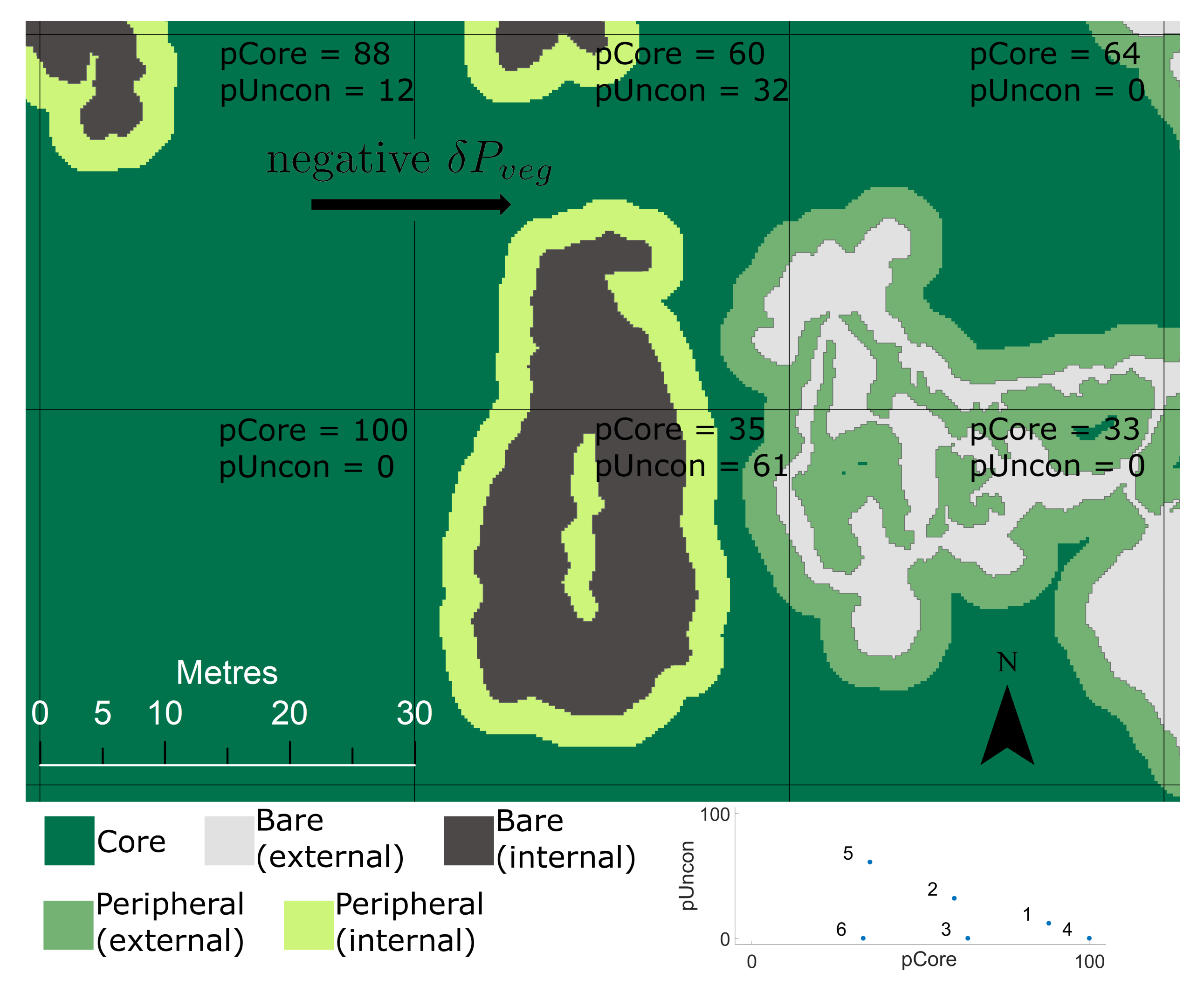
2.3.3. Integrity of Marsh Platform

The first morphological metric describes the integrity of the marsh platform by the proportion of each 30 m satellite pixel’s area that contains undissected vegetated marsh areas. It is referred to as pCore.

The Morphological Spatial Pattern Analysis (MSPA—[39]) tool, supplied within the GUIDOS toolbox [40], is a morphological segmentation algorithm designed to assess habitat connectivity and fragmentation—for example, in forest ecosystems [41,42] or for planning of green infrastructure [43]. MSPA operates on a binary raster of ‘foreground’ and ‘background’ pixels, where foreground represents the habitat or land cover type of interest. It classifies foreground pixels according to how many other foreground pixels they are adjacent to and a distance parameter controlling the width of areas considered to be ‘egde’ because they are close to background pixels. Pixels are allocated to one of seven foreground classes (core, edge, perforation, bridge, loop, branch, and islet) and a background class. Each of these classes can also have an attribute describing whether it is entirely surrounded by other foreground classes (internal) or with connectivity through adjacent background classes to the edge of the raster (external). Loops and bridges can additionally be defined as appearing independently or within edges or perforations. The result is 22 possible types of feature that are extracted from the binary raster. In this context, foreground pixels represent vegetated marsh platform areas while background pixels correspond to bare sediments, channels, and pools. Although these classes were originally designed to describe habitat connectivity features, analogues can be readily defined for most classes in the context of fine-scale saltmarsh morphology (

Table 1. Outline of the landform classes produced by MSPA and their interpretation in the context of fine-scale salt marsh morphology (internal: no background connectivity to raster edge; external: background connectivity to raster edge).

Feature	Classification Rule	Interpretation
Background	Background pixels	Salt pans or pools if internal, channel or mudflat if external
Core	Areas greater than the edge distance from nearest background pixel	Large, coherent marsh areas
Edge	Areas within the edge distance of background pixels	Margins of core areas with channel connectivity
Perforation	Edge pixels entirely enclosing an area of background pixels	Margins of salt pans or pools without channel connectivity
Branch	Strip less than twice the edge distance wide that joins to a core area at one end	Narrow extensions from core areas
Islet	Foreground area too small to contain any core area	Small, isolated marsh fragments
Bridge	Strip less than twice the edge distance wide that joins two core areas	Narrow causeway between larger coherent marsh areas
Bridge in Edge	Bridge joining two areas of edge class	As above but for edge areas
Bridge in Perforation	Bridge joining two areas of perforation class	Narrow strip of marsh separating marsh areas that are distinct but entirely contained within a salt pan or pool
Loop	Strip less than twice the edge distance wide that joins to the same core area at both ends	Narrow strip of marsh enclosing a salt pan or pool
Loop in Edge	Strip less than twice the edge distance wide that joins to the same edge area at both ends	Narrow strip of marsh enclosing a salt pan or pool
Loop in Perforation	Strip less than twice the edge distance wide that joins to the same perforation area at both ends	Narrow strip of marsh enclosing a smaller salt pan or pool within a larger one

). MSPA was applied to a 25 cm-resolution binary raster derived from the Environment Agency’s salt marsh extents layer [17], which describes recent (2008–2010) marsh morphology. Core areas were defined as parts of vegetated marsh greater than the MSPA edge width parameter (2.5 m) from a background area. The pCore metric was the aggregation of both internal and external MSPA ‘core’ classes for a given satellite pixel area.

2.3.4. Limitations to Tidal Connectivity

The second morphological metric describes the proportion of pixel area comprised of unvegetated areas and their periphery that are unconnected to the drainage network; it is denoted pUncon. It is also derived from the MSPA segmentation and reflects pools or pans and their periphery that do not have connectivity via channels to the offshore domain. The pUncon metric was computed as the aggregation of the ‘internal’ MSPA classes, including unvegetated areas.

An example area of the MSPA segmentation for six adjacent satellite pixels is shown in Figure 4, with the respective values for the pCore and pUncon metrics. These two morphological metrics are interpreted as describing the marsh morphology within a data-space that separates, at its extremes, between contiguous, undissected marsh platform (high pCore), marsh areas that are heavily fragmented by creek networks (low pCore, low pUncon), and areas that have a high density of salt pans and pools (low pCore, high pUncon). The inset graph on Figure 4 illustrates the position of the depicted pixels within this data-space. The processes leading to these morphologies are likely to be different, as are their likely future evolutionary trajectories. Creek networks, particularly low-order ones, are typically stable in the platform once established [44], and maintain a dynamic equlibrium with the tidal prism [45]. Interior areas of intact marsh platforms may remain so or become punctuated by pools or pans [46,47,48], with the density of pans being related to the tidal range and sediment type at a national scale in the UK [49] and the elevation and distance from marsh edge at a site scale [47].

2.4. Probability of Observing Marsh Degradation

Marsh degradation was considered to have occurred for pixels where the $\delta P_{veg}$ was negative. For each of the topological and morphological metrics, the probability of a location exhibiting degradation was computed from the proportion of pixels where $\delta P_{veg}<0$ in each of 100 equal intervals across the observed ranges of the four topological or morphological metrics described above (CD, ED, pCore, pUncon). Least-squares regression analyses were used to establish relationships for each of the metrics between the observed probabilities of degradation and interval centre points.

3. Results

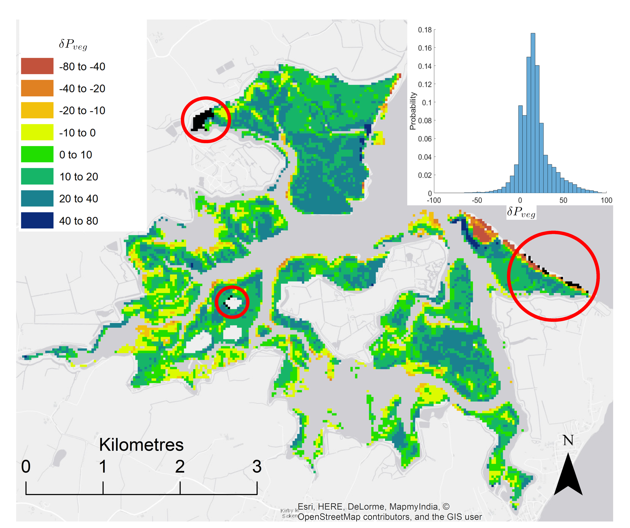
3.1. Morphodynamic Change

$\delta P_{veg}$ was estimated for approximately 180,000 30 m pixels, amounting to approximately 16,200 ha of marsh. An example of the resulting metric for about 600 ha of salt marsh in Hamford Water, Essex, is presented in Figure 5 to illustrate the degree of spatial variability observed in changes to marsh integrity over relatively small spatial scales. The inset histogram shows the distribution of estimates across the entire study domain from the Humber to the Thames, which can be seen to be normal but with a mean somewhat above zero, suggesting a dominance of vegetation establishment within the domain, even though this is not necessarily evident within the Hamford Water subset depicted. The overall probability of degradation for the entire dataset was 0.144 for the approximate time period 1985–2016.

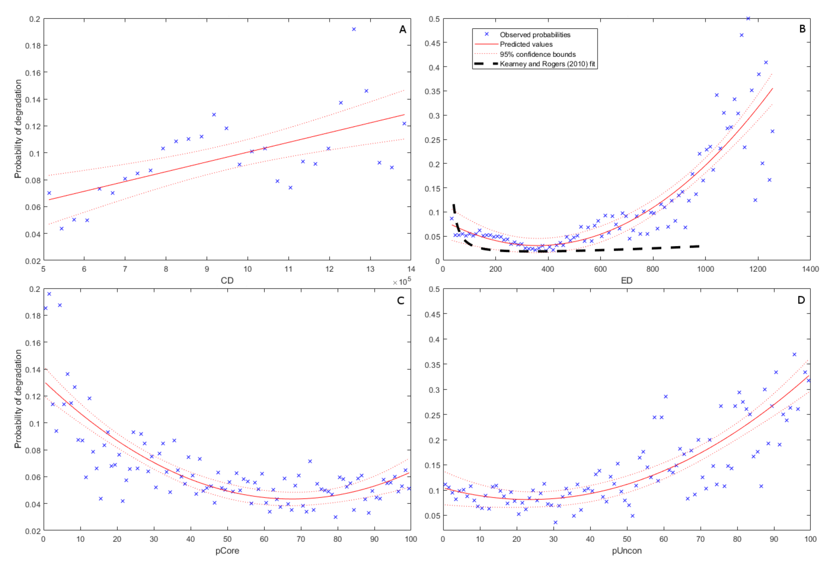
3.2. Topological and Morphological Relationships

No significant regression relationship was found between Cost Distance (CD) and the probability of degradation when using the entire dataset. The CD parameter, however, has very long tails to its distribution, particularly at the upper end of the scale. At the lower end, these pixels represent the seaward limit of open-coast marsh areas, while at the upper end they are mainly high, supratidal regions towards the heads of estuaries or around islands of high ground. These locations may not be expected to experience the same controls on marsh morphodynamics as the majority of interior and estuarine marsh areas, so might confound the regression analysis for such areas. Areas with exceptionally low CD values coincide with the seaward margins of open coast marshes, which have the potential to retreat [14] and advance rapidly [24]. Values of $\delta P_{veg}$ in such areas therefore tend towards extreme values and reflect changes in marginal position more than changes in marsh platform integrity. Where CD is exceptionally high, $\delta P_{veg}$ values are associated with the upland boundary and may again not reflect changes in marsh platform integrity but rather shifts between terrestrial and halophytic vegetation communities, which may have completely different reflectances. The extremities of the CD distribution were discarded where $CD\le$ 500,000 and $CD\ge$ 1,400,000. 91% of the population was retained, and all the locations excluded within Hamford Water are marked, for illustration purposes, as black pixels within the red circles on Figure 5. With the extremities of the distribution excluded, a significant positive linear relationship between CD and the probability of degradation was found (Adjusted $R^2=0.37$, $p\le 0.001$—see Figure 6, Panel A). The low positive coefficient suggests that, as CD increases—implying a reduction in tidal connectivity to offshore waters—the probability of marsh degradation increases slightly. CD values do not represent real-world physical quantities. For instance, a doubling of CD could occur because of multiple different combinations of increased horizontal distance and/or elevation. The precise coefficients of this relationship are therefore not readily interpretable beyond their sign and approximate magnitude.

A second-order polynomial relationship was found between Euclidean Distance (ED) and the probability of degradation, whereby areas with a low ED exhibit moderate probabilities of degradation in the order of 0.1, with this probability declining to a minimum of less than 0.05 at around 350 m before increasing again with ED to values in excess of 0.3 at distances of 1200 m. The relationship is significant at $p\le 0.001$, and the high adjusted $R^2$ of 0.76 suggests that ED is an important determinant of changes in condition (Figure 6, Panel B). The ED metric is directly comparable to that used by Kearney and Rogers [20] to predict changes in marsh condition, and the regression fit from their study is superimposed on the figure for comparison.

Significant relationships were also found between both pCore and pUncon and the probability of degradation (Figure 6, panels C and D, respectively). The former relationship implies a decrease in the probability of degradation with increasing values of the pCore, although very high values of pCore become associated with increased probabilities of degradation again. With high adjusted $R^2$ values of 0.63 for pCore, the proportion of a pixel that is core vegetated marsh area is strongly related to changes in marsh condition. Pixels containing salt pan features were relatively rare within the dataset, with n = 13,157, representing 9.2% of all pixels. The regression only included those pixels where pUncon $>0$. The relationship is significant with an $R^2$ value of 0.63, suggesting a strong positive relationship between the proportion of an area that comprises salt pans and their peripheral marsh features and the history of morphological evolution.

Summaries of all four regression relationships are provided in

Table 2. Summary of regression models between topological or morphological metrics and the probability of marsh degradation.

	Adjusted ${\mathit{R}}^2$	x	${\mathit{x}}^2$	f-Stat	p-Value
CD	0.37	7.3 $\times {10}^{-8}$	N/A	17.4	≤0.001
ED	0.76	−2.9 $\times {10}^{-4}$	4.0 $\times {10}^{-7}$	147	≤0.001
pCore	0.63	−2.6 $\times {10}^{-3}$	1.9 $\times {10}^{-5}$	85.7	≤0.001
pUncon	0.63	−2.0 $\times {10}^{-3}$	−4.2 $\times {10}^{-5}$	83.9	≤0.001

.

4. Discussion

4.1. Morphodynamic Change

The regional data for the Humber to Thames study area show an overall trend towards increasing marsh platform integrity over time, with rapid increases in integrity being much more common than rapid losses (inset to Figure 5). This pattern is, in part, a result of the rapid infilling and marsh advance that occurred in The Wash embayment during the observation period (1985–2016), where rates of margin advance up to 75 m per year were observed between 1992 and 2014 [24]. This established a large area of marsh that is included in the analysis and is associated with very high values of $\delta P_{veg}$. The pattern of increase and decrease in internal platform integrity is much patchier elsewhere, as seen for Hamford Water (Figure 5).

A degree of bias towards positive values of $\delta P_{veg}$ was introduced by the choice of a marsh presence/absence mask from relatively late in the study period. Phelan et al. [17] base their mapping on data from 2008 to 2010. This implies that areas that may have contained marsh early in the study period, but which became completely unvegetated prior to 2008 and would produce negative $\delta P_{veg}$, will have been excluded from the analysis. A visual assessment of the aerial photography from 2013/14 and 1992 suggests that this phenomenon was rare within the region. The scale of negative changes in the overall horizontal extent of the marshes over the study period, relative to the Landsat pixel size, is typically small. Only isolated pixels at the seaward limits of some open-coast marshes are likely to have been affected by this bias [24]. Our findings support the idea that vegetated areas of marsh platform have the potential to increase in platform integrity much more rapidly than they deteriorate. This is likely the result of the potential for the rapid colonisation of large horizontal extents of unvegetated surfaces that accrete to a critical elevation to support seedling survival [29] near-simultaneously because of their very low gradients. Conversely, during erosive phases sediment loss is likely to be more gradual due to biostabilisation [50,51], and is also likely to be more localised in areas of high hydrodynamic stress. Assuming that morphological change can be inferred from vegetation extent change, the data suggest that, in marsh interiors at least, accretionary processes tend to outpace erosional ones.

We address change over a single time period only. Our methodology is not, therefore, able to detect regime shifts or abrupt changes as distinct from more gradual trends that result in the same $\delta P_{veg}$ value. A natural development of our work, as the data archives become longer and denser, would be to incorporate temporal segmentation approaches similar to those used by the LandTrendr algorithm [52,53]. This would allow us to investigate whether the topological and morphological controls on abrupt regime shifts differ from those on gradual changes. Such work is beyond the scope of the current study.

4.2. Geomorphic Setting (CD)

No significant relationship was found when considering probability of degradation across the entire range of CD. This is likely because CD has a large range between 3.9 $\times {10}^5$ and 3.1 $\times {10}^6$, with over 90% of values falling in the interval 5.0 $\times {10}^5$ and 1.4 $\times {10}^6$. The upper end of the distribution in particular is therefore very sparse. This leads to very small numbers of pixels being represented in each of the 100 intervals across the CD distribution. With the relatively low prevalence of degradation in the order of 10% within the entire dataset, these small samples at high CD values often fail to represent any degraded pixels, resulting in probabilities of degradation of zero. Even if some degraded pixels are sampled, the resulting probability estimate is unlikely to be usefully precise while the sample size remains below about 50 pixels. Furthermore, the areas where CD $>1.4\times {10}^6$ are typically high-elevation areas which are likely to be supratidal and may therefore be expected to be responding to different processes controlling their dynamics when compared to the intertidal marsh areas that are of principal interest here. Similarly, the data density is very low where $CD<5.0\times {10}^5$, as these areas represent the seaward limits of open-coast marshes. The observations in these areas are likely to be dominated by the wave-driven erosion of the marsh margin rather than the internal marsh changes that $\delta P_{veg}$ represents. The probabilities of degradation in these areas are relatively high, aligning well with the observations of the widespread retreat of open coast marsh margins in the region [24]. Excluding such areas from the analysis is therefore justifiable, as it enables insight into dynamics in the intertidal zone that are otherwise masked by variance in other areas that are either artefactual or likely to arise from a different suite of processes to those types of marsh interior processes that this study seeks to assess.

When the range of CD was limited to the interval $5.0\times {10}^5$ and $1.4\times {10}^6$, the regression analysis showed a significant positive linear relationship between CD and the probability of a pixel showing degradation. Low CD values are associated with minimum probabilities of degradation (Panel A, Figure 6). This implies that the interiors of open-coast marshes experience little degradation, while those towards the head of estuaries or tidal inlets are more susceptible. This aligns well with the conceptualisation of sediment sources for this study region, which is dominated by minerogenic marshes [26] and offshore tidal waters are the primary source of allochthonous inputto support marsh elevations [54]. Those areas of marsh that are least tidally connected (high CD) are shown to be the most vulnerable, since the delivery of sediments is most restricted in these areas. This finding contrasts with those of Kearney and Rogers [20], who observe an increasing probability of degradation at shorter distances up-estuary. This is because the domain that they studied on the east coast of the US has much more significant riverine inputs and the locations of sedimentation are therefore fluvially, rather than tidally, dominated. Additionally, the Chesapeake Bay (US) marshes are highly organogenic, with the upper marsh sediment total organic content being reported to be around 80% at Rhode River [55], which implies that autochthonous accumulation dominates. By comparison, the UK east coast marshes rely more heavily on allochthonous inputs with much lower total organic contents than those of the US, at around 15% [56]. The relationship we find between CD and the probability of degradation is relatively weak ($R^2=0.37$), reflecting the fact that other factors, likely occurring at smaller scales, may be more significant. These may include the controls represented by the other ED, pCore, and pUncon metrics in this study, but also factors such as proximity and the magnitude of fluvial sediment loads that we have been unable to address here. The strength of the relationship may also arise, in part, from the failures of the simplified CD metric to perfectly represent tidal connectivity within the domain. Nevertheless, given the size of the region considered, the heterogeneity of marsh settings represented and the methodological limitations, the fact that any relationship emerges implies that the position of a marsh within the wider coastal setting is an important control on its vulnerability to sediment starvation and subsequent degradation. The contrast between our findings and those of Kearney and Rogers [20] suggests that the marsh position is not, however, a diagnostic parameter, since its effect varies between regions. Rather, it modulates the impacts of larger-scale geomorphological contexts (that may be considered as boundary conditions at the scale of the analysis presented here), such as sediment sources and delivery pathways. This finding implies that empirical attempts to predict morphological change in coastal wetlands must be nested within a hierarchy of process understanding in order to ensure that outcomes are appropriate for a particular location. Not all regions behave equally.

4.3. Distance from Creek/Edge of Marsh Parcel (ED)

The relationship established between Euclidean Distance (ED) and probability of degradation is significant and stronger ($R^2=0.76$) than that found for CD. It is also non-linear with initially high probabilities at short distances that decline to a minimum around 350 m before increasing dramatically. There is a notable similarity with the relationship observed in Chesapeake and Delaware Bays (black dashed line on Figure 6). The initial decline observed here is somewhat less rapid than that found by Kearney and Rogers [20], and beyond 400 m there is a strong increase in the probability of degradation with increasing ED at a rate that exceeds that found by Kearney and Rogers [20].

The inter-regional similarity observable regarding ED suggests that topological factors controlling marsh stability at scales below those represented by CD (i.e., within-marsh scales rather than within-estuary scales) may be operating in very similar fashions between regions, although the differences in the rates of decline and increases in degradation probability around the 350 m minima suggest a possible dependence on the scale/size of the marsh systems being observed. Marsh parcels are substantially smaller in the UK than in the USA example, where ED values of up to about 100 km were observed, although the goodness of fit above about 1 km declines. Differences in drainage network morphologies may also contribute. For the context of the east coast of the UK, the initial decline in probabilities can be interpreted, in part, as a function of the scale of channel identified in the basemap used for the distance calculations. Only major creeks exceeding 42.5 m width were included. Where the ED values are very low, the degradation measured by $\delta P_{veg}$ could have a component that reflects the marginal erosion of the banks of large channels, where fetch is sufficient for wave-driven erosion to become significant in determining the spectral change within the pixel over the study period. Thereafter, however, it still appears that marsh vulnerability decreases with increasing distance from these major channels. This could be associated with the increasing drainage density of smaller creeks (not resolved by the ED metric used here), leading to shorter unchannelised lengths, a greater preponderance of levee-effects [19], and ultimately a greater potential for the drainage of and allochthonous sediment import to marsh areas within 350 m of a major channel. Beyond this distance, the probability of degradation increases again, which we attribute to declining drainage density and efficiency, leading to decreasing potential for tidal flushing, drainage, and sediment import as distances from the primary tidal channels continue to increase. Internal marsh areas without efficient drainage and a long way from major channels tend to experience relatively little elevation gain from external sources [57] and, particularly in the context of relative sea level rise, vegetation experiences increasing water and salt stress, potentially leading to die-back and substrate collapse [58]. This phenomenon is observable within the region and is illustrated by the hotspots of negative $\delta P_{veg}$ in marsh interior areas shown in Figure A1 within the Appendix A.

4.4. Percentage Core Areas (pCore)

pCore is based on a 25 cm spatial resolution and therefore resolves differences in marsh morphology at a sub-pixel scale in terms of $\delta P_{veg}$. The same is true for pUncon. The relationship observed whereby the probability of degradation decreases to a minimum at pCore values of around 70% before levelling off or increasing slightly implies that fragmented areas of marsh (low pCore) reflect a history of greater marsh degradation. This implies that more degraded areas of marsh may continue to degrade at a faster rate than areas of platform with a high integrity. As a marsh platform becomes fragmented, pCore declines and the perimeter–area ratio of the remaining marsh parcels increases, providing a greater effective marginal length that may be vulnerable to erosion by hydrodynamic forces. The stability of the morphological state therefore decreases with increasing fragmentation, representing a positive morphodynamic feedback controlling marsh degradation. The slight increase in probability at very high pCore values may reflect the tendency for marsh areas that are separated from minor creeks by only a few metres to begin to degrade as a result of water stress [58], which Ursino et al. [59] showed can increase rapidly away from channels. Additional contributors to marsh degradation occurring at high pCore values may be reduced sediment inputs [19,57] or increased salt stress [60] in the interiors of marsh parcels.

4.5. Percentage of Unconnected Areas (pUncon)

The relationship between pUncon and the probability of degradation is significant, with a $R^2$ value of 0.63. The form of the relationship takes an almost opposite form to that for pCore, with higher values of pUncon being associated with higher probabilities of degradation. pCore and pUncon are somewhat negatively correlated to each other (R = −0.11, p ≤ 0.001), so this inverse relationship may in part reflect the same processes as are discussed with reference to pCore. The analysis for pUncon, however, incorporates only those marsh pixels where pans or pools are present, which represents a small subset of the dataset (9.2%). As such, this analysis allows for the isolation of behaviours exclusively in areas where pans are observed. Areas with a higher pUncon and therefore a greater proportion of pan-related features exhibit higher probabilities of degradation. Notably, for fragmentation identified by the pUncon metric, the maximum probabilities of degradation observed are much higher (≈0.5) than those calculated on the larger dataset of pCore (≈0.2), where low metric values also indicate fragmentation. Low pCore values, by contrast, largely reflect fragmentation by creek networks and bare surfaces connected to them. The difference in magnitudes of probability identified by the two regression relationships implies that the presence of pans indicates a much more vulnerable landscape configuration than one fragmented by creeks. Neumeier et al. [61] identified the life cycle of pans in Canadian marshes whereby they undergo a phase of active expansion before achieving maturity. The data presented here also support the conclusion that pans have a tendency to expand over decadal timescales. The analysis cannot identify causality, however. It is possible that the presence of pans establishes a feedback encouraging their subsequent expansion as the marsh develops [48]. Questions also remain over the causes of initial pan formation, with some theories suggesting that event-based phenomena, such as smothering of vegetation by rafted debris, may cause pans to develop. French et al. [62] noted that pan densities are lower on the more enclosed of the backbarrier marshes in Norfolk, where less debris may be rafted into the marshes over shorter seaward margins. Their finding is correlative but Pethick [47] argues that a mechanism for pan initiation on mature marshes must exist. Whatever the cause of pan initiation, our findings suggest that, once established, marsh areas containing pans are highly vulnerable compared to other areas. It is possible, therefore, that stochastic events, such as debris rafting, could initiate a long-term landscape vulnerability. In contrast, pans may simply be diagnostic of other conditions such as relative sea level changes, tidal range, or coastal configuration, rather than morphodynamic drivers in their own right [49]. If pans are not, in themselves, morphodynamic drivers, then our findings would suggest that the external controls causing pan formation continue to cause subsequent expansion and the conclusion that panned landscapes are vulnerable stands. Further work is needed to address the question of controls on salt pan development to better understand the fundamental causes of this vulnerability.

5. Conclusions

Our findings show that there exist certain overarching controls on the vulnerability of salt marshes to degradation at a range of scales. We demonstrate this observation through the application of a systematic spatial analysis of a simple, satellite-image-derived measure of change. By applying this methodology at the regional scale and across a range of estuarine, backbarrier, embayment, and open coast settings, we illustrate the nature of these controls more clearly than has hitherto been possible.

This work has presented an inherently scalable method for monitoring the platform integrity of salt marsh surfaces at a sub-pixel scale that is easily adapted to incorporate current and future data sources (such as imagery from the more recently launched Sentinel 2 satellites). The $\delta P_{veg}$ metric presented here is a continuous variable representing change in marsh surface integrity over a given time period. It therefore provides substantially more statistical possibilities than the MSCI [20] or than we have explored in this study.

We express topological and morphological factors at a range of scales as metrics describing the connectivity of tidal waters, position within marsh, marsh platform integrity, and the prevalence of salt pans or pools. We demonstrate that all of these are significantly related to the morphodynamic evolution of marshes. This spatial hierarchy of morphological controls may continue to be applicable at both larger and smaller scales than are addressed here. The presence of controls at larger scales is shown by the finding of contrasting relationships between geomorphic setting and marsh degradation in this study and that of [20]. We hypothesise that this difference arises from regional-scale contrasts in climate, biota, sediment supply, and sea-level history that cause fundamental differences in the processes by which the marsh systems function and evolve. At a whole-marsh scale, however, responses to the distance from the marsh margin seem to be fairly consistent between regions, suggesting commonality in some of the processes governing marsh dynamics. At a smaller scale than is considered here, a variety of factors may become important, such as the spatial distribution of vegetation types [46,63] or phenotypes [64], which may determine sediment erodibility.

We have presented aggregated relationships that emerge at a regional scale. Overall, these suggest that marsh areas that are already exhibiting some form of fragmentation that lie far from the nearest creek and towards the heads of estuaries and inlets are the most likely to exhibit degradation. The prediction of changes in a particular location remains challenging. No relationships were found between the continuous values of $\delta P_{veg}$ itself and any of the predictors presented here using basic statistical techniques. Only when the dimensionality of the dataset is reduced to probabilities do aggregated relationships emerge. The large number of parameters influencing marsh dynamics, the multiple scales of processes involved, and the complex interactions between them means that statistical prediction of internal marsh changes will require methods capable of capturing the interactions and high dimensionality that are inherent to such natural systems. Further work is needed to explore the potential of more sophisticated statistical techniques drawn from machine learning domains to synthesise datasets such as the one presented here into location-specific values of parameters describing the sign and magnitude of predicted marsh evolution.

References

1. McOwen, C.; Weatherdon, L.; Bochove, J.W.; Sullivan, E.; Blyth, S.; Zockler, C.; Stanwell-Smith, D.; Kingston, N.; Martin, C.; Spalding, M.; et al. A global map of saltmarshes. Biodivers. Data J. 2017, 5, e11764. [Google Scholar] [CrossRef]
2. Friess, D.A.; Yando, E.S.; Alemu I, J.B.; Wong, L.W.; Soto, S.D.; Bhatia, N. Ecosystem Serices and Dissserices of Mangrove Forests and Salt Marshes. In Oceanography and Marine Biology: An Annual Review; CRC Press: Boca Raton, FL, USA, 2020; pp. 58:107–58:142. [Google Scholar]
3. Mitsch, W.J.; Gosselink, J.G. Wetlands, 3rd ed.; Wiley: New York, NY, USA, 2000; p. 920. [Google Scholar]
4. McLeod, E.; Chmura, G.L.; Bouillon, S.; Salm, R.; Björk, M.; Duarte, C.M.; Lovelock, C.E.; Schlesinger, W.H.; Silliman, B.R. A blueprint for blue carbon: Toward an improved understanding of the role of vegetated coastal habitats in sequestering CO2. Front. Ecol. Environ. 2011, 9, 552–560. [Google Scholar] [CrossRef] [Green Version]
5. Möller, I.; Spencer, T.; French, J.R.; Leggett, D.J.; Dixon, M. Wave transformation over salt marshes: A field and numerical modelling study from North Norfolk, England. Estuarine Coast. Shelf Sci. 1999, 49, 411–426. [Google Scholar] [CrossRef]
6. Möller, I. Quantifying saltmarsh vegetation and its effect on wave height dissipation: Results from a UK East coast saltmarsh. Estuarine Coast. Shelf Sci. 2006, 69, 337–351. [Google Scholar] [CrossRef]
7. Burden, A.; Garbutt, R.; Evans, C.; Jones, D.; Cooper, D. Carbon sequestration and biogeochemical cycling in a saltmarsh subject to coastal managed realignment. Estuarine Coast. Shelf Sci. 2013, 120, 12–20. [Google Scholar] [CrossRef] [Green Version]
8. Chmura, G.L. What do we need to assess the sustainability of the tidal salt marsh carbon sink? Ocean. Coast. Manag. 2013, 83, 25–31. [Google Scholar] [CrossRef]
9. Roner, M.; Alpaos, A.D.; Ghinassi, M.; Marani, M.; Silvestri, S.; Franceschinis, E. Spatial variation of salt-marsh organic and inorganic deposition and organic carbon accumulation: Inferences from the Venice lagoon, Italy. Adv. Water Resour. 2016, 93, 276–287. [Google Scholar] [CrossRef]
10. Boesch, D.F.; Turner, R.E. Dependence of fishery species on salt marshes: The role of food and refuge. Estuaries 1984, 7, 460. [Google Scholar] [CrossRef]
11. Costa, M.J.; Costa, J.; de Almeida, P.R.; Assis, C.A. Do eel grass beds and salt marsh borders act as preferential nurseries and spawning grounds for fish? An example of the Mira estuary in Portugal. Ecol. Eng. 1994, 3, 187–195. [Google Scholar] [CrossRef]
12. Ladd, C.J.; Duggan-Edwards, M.F.; Bouma, T.J.; Pagès, J.F.; Skov, M.W. Sediment Supply Explains Long-Term and Large-Scale Patterns in Salt Marsh Lateral Expansion and Erosion. Geophys. Res. Lett. 2019, 46, 11178–11187. [Google Scholar] [CrossRef] [Green Version]
13. Hughes, R.G.; Paramor, O.A.L. On the loss of saltmarshes in south-east England and. J. Appl. Ecol. 2004, 41, 440–448. [Google Scholar] [CrossRef]
14. van der Wal, D.; Pye, K. Patterns, rates and possible causes of saltmarsh erosion in the Greater Thames area (UK). Geomorphology 2004, 61, 373–391. [Google Scholar] [CrossRef]
15. Burd, F. Erosion and Vegetation Change on the Salt Marshes of Essex and North Kent between 1973 and 1988; Technical Report; Nature Conservancy Council: Peterborough, UK, 1992. [Google Scholar]
16. Cooper, N.J.; Cooper, T.; Burd, F. 25 years of salt marsh erosion in Essex: Implications for coastal defence and nature conservation. J. Coast. Conserv. 2001, 7, 31–40. [Google Scholar] [CrossRef]
17. Phelan, N.; Shaw, A.; Baylis, A. The Extent of Saltmarsh in England and Wales: 2006–2009; Environment Agency: Bristol, UK, 2011. [Google Scholar]
18. Vandenbruwaene, W.; Meire, P.; Temmerman, S. Formation and evolution of a tidal channel network within a constructed tidal marsh. Geomorphology 2012, 151–152, 114–125. [Google Scholar] [CrossRef]
19. French, J.R.; Spencer, T. Dynamics of sedimentation in a tide-dominated backbarrier salt marsh, Norfolk, UK. Mar. Geol. 1993, 110, 315–331. [Google Scholar] [CrossRef]
20. Kearney, M.S.; Rogers, A.S. Forecasting sites of future coastal marsh loss using topographical relationships and logistic regression. Wetl. Ecol. Manag. 2010, 18, 449–461. [Google Scholar] [CrossRef]
21. Allen, J. Simulation models of salt-marsh morphodynamics: Some implications for high-intertidal sediment couplets related to sea-level change. Sediment. Geol. 1997, 113, 211–223. [Google Scholar] [CrossRef]
22. Da Lio, C.; D’Alpaos, A.; Marani, M. The secret gardener: Vegetation and the emergence of biogeomorphic patterns in tidal environments. Philos. Trans. Ser. Math. Phys. Eng. Sci. 2013, 371. [Google Scholar] [CrossRef] [Green Version]
23. D’Alpaos, A.; Lanzoni, S.; Marani, M.; Rinaldo, A. Landscape evolution in tidal embayments: Modeling the interplay of erosion, sedimentation, and vegetation dynamics. J. Geophys. Res. Earth Surf. 2007, 112, 1–17. [Google Scholar] [CrossRef] [Green Version]
24. Evans, B.R.; Möller, I.; Spencer, T.; Smith, G. Dynamics of salt marsh margins are related to their three-dimensional functional form. Earth Surf. Process. Landforms 2019, 44, esp.4614. [Google Scholar] [CrossRef]
25. Pethick, J.; Leggett, D. The morphology of the Anglian coast. In Coastlines of the Southern North Sea; Hillen, R., Verhagen, H., Eds.; American Society of Civil Engineers (ASCE): Reston, VA, USA, 1993; pp. 52–64. [Google Scholar]
26. Pye, K.; French, P. Erosion and Accretion Processes on British Saltmarshes: Volume Three; Technical Report; Cambridge Environmental Research Consultants: Cambridge, UK, 1993. [Google Scholar]
27. Allen, J. Morphodynamics of Holocene salt marshes: A review sketch from the Atlantic and Southern North Sea coasts of Europe. Quat. Sci. Rev. 2000, 19, 1155–1231. [Google Scholar] [CrossRef]
28. Kestner, F. The Old Coastline of the Wash. T Geogr. J. 1962, 128, 457–471. [Google Scholar] [CrossRef]
29. Balke, T.; Stock, M.; Jensen, K.; Bouma, T.J.; Kleyer, M. A global analysis of the seaward salt marsh extent: The importance of tidal range. Water Resour. Res. 2016, 52, 3775–3786. [Google Scholar] [CrossRef] [Green Version]
30. Suchrow, S.; Jensen, K. Plant species responses to an elevational gradient in German North Sea salt marshes. Wetlands 2010, 30, 735–746. [Google Scholar] [CrossRef]
31. Ganju, N.K.; Defne, Z.; Kirwan, M.L.; Fagherazzi, S.; D’Alpaos, A.; Carniello, L. Spatially integrative metrics reveal hidden vulnerability of microtidal salt marshes. Nat. Commun. 2017, 8, 14156. [Google Scholar] [CrossRef] [Green Version]
32. Gorelick, N.; Hancher, M.; Dixon, M.; Ilyushchenko, S.; Thau, D.; Moore, R. Google Earth Engine: Planetary-scale geospatial analysis for everyone. Remote Sens. Environ. 2017, 202, 18–27. [Google Scholar] [CrossRef]
33. Lopes, C.L.; Mendes, R.; Caçador, I.; Dias, J.M. Assessing salt marsh extent and condition changes with 35 years of Landsat imagery: Tagus Estuary case study. Remote Sens. Environ. 2020, 247, 111939. [Google Scholar] [CrossRef]
34. Hargrove, W.W.; Hoffman, F.M.; Hessburg, P.F. Mapcurves: A quantitative method for comparing categorical maps. J. Geogr. Syst. 2006, 8, 187–208. [Google Scholar] [CrossRef]
35. ABPMer. Atlas of Marine Energy Resources. 2008. Available online: http://www.renewables-atlas.info/ (accessed on 5 May 2015).
36. French, J. Tidal marsh sedimentation and resilience to environmental change: Exploratory modelling of tidal, sea-level and sediment supply forcing in predominantly allochthonous systems. Mar. Geol. 2006, 235, 119–136. [Google Scholar] [CrossRef]
37. French, J.R.; Spencer, T.; Murray, A.L.; Arnold, N.S. Geostatistical analysis of sediment deposition in two small tidal wetlands, Norfolk, UK. J. Coast. Res. 1985, 11, 308–321. [Google Scholar]
38. Reed, D.J.; Spencer, T.; Murray, A.L.; French, J.R.; Leonard, L. Marsh surface sediment deposition and the role of tidal creeks: Implications for created and managed coastal marshes. J. Coast. Conserv. 1999, 5, 81–90. [Google Scholar] [CrossRef]
39. Soille, P.; Vogt, P. Morphological segmentation of binary patterns. Pattern Recognit. Lett. 2009, 30, 456–459. [Google Scholar] [CrossRef]
40. Vogt, P. GUIDOS: Tools for the assessment of pattern, connectivity, and fragmentation. In Proceedings of the EGU General Assembly 2013, Vienna, Austria, 7–12 April 2013; Volume 15, p. 13526. [Google Scholar]
41. Ostapowicz, K.; Vogt, P.; Riitters, K.H.; Kozak, J.; Estreguil, C. Impact of scale on morphological spatial pattern of forest. Landsc. Ecol. 2008, 23, 1107–1117. [Google Scholar] [CrossRef]
42. Saura, S.; Vogt, P.; Velázquez, J.; Hernando, A.; Tejera, R. Key structural forest connectors can be identified by combining landscape spatial pattern and network analyses. For. Ecol. Manag. 2011, 262, 150–160. [Google Scholar] [CrossRef]
43. Chang, Q.; Liu, X.; Wu, J.; He, P. MSPA-Based Urban Green Infrastructure Planning and Management Approach for Urban Sustainability: Case Study of Longgang in China. J. Urban Plan. Dev. 2015, 141, A5014006. [Google Scholar] [CrossRef]
44. French, J.R.; Stoddart, D.R. Hydrodynamics of saltmarsh creek systems: Implications for marsh morphological development and material exchange. Earth Surf. Process. Landforms 1992, 17, 235–252. [Google Scholar] [CrossRef]
45. Friedrichs, C.T.; Perry, J.E. Tidal salt marsh morphodynamics: A synthesis. J. Coast. Res. 2001, 27, 7–37. [Google Scholar]
46. Adam, P. Saltmarsh Ecology; Cambridge University Press: Cambridge, UK, 1990; p. 461. [Google Scholar]
47. Pethick, J. The distribution of salt pans on tidal salt marshes. J. Biogeogr. 1974, 1, 57–62. [Google Scholar] [CrossRef]
48. Yapp, R.H.; Johns, D.; Jones, O.T. The salt marshes of the Dovey Estuary. J. Ecol. 1917, 5, 65–103. [Google Scholar] [CrossRef]
49. Goudie, A. Characterising the distribution and morphology of creeks and pans on salt marshes in England and Wales using Google Earth. Estuarine Coast. Shelf Sci. 2013, 129, 112–123. [Google Scholar] [CrossRef]
50. Murray, A.B.; Knaapen, M.A.; Tal, M.; Kirwan, M.L. Biomorphodynamics: Physical-biological feedbacks that shape landscapes. Water Resour. Res. 2008, 44. [Google Scholar] [CrossRef]
51. Spencer, T.; Möller, I.; Rupprecht, F.; Bouma, T.J.; van Wesenbeeck, B.K.; Kudella, M.; Paul, M.; Jensen, K.; Wolters, G.; Miranda-Lange, M.; et al. Salt marsh surface survives true-to-scale simulated storm surges. Earth Surf. Process. Landforms 2016, 41. [Google Scholar] [CrossRef]
52. Kennedy, R.E.; Yang, Z.; Cohen, W.B. Detecting trends in forest disturbance and recovery using yearly Landsat time series: 1. LandTrendr—Temporal segmentation algorithms. Remote Sens. Environ. 2010, 114, 2897–2910. [Google Scholar] [CrossRef]
53. Kennedy, R.; Yang, Z.; Gorelick, N.; Braaten, J.; Cavalcante, L.; Cohen, W.; Healey, S. Implementation of the LandTrendr Algorithm on Google Earth Engine. Remote Sens. 2018, 10, 691. [Google Scholar] [CrossRef] [Green Version]
54. Reed, D.J. Sediment dynamics and deposition in a retreating coastal salt marsh. Estuarine Coast. Shelf Sci. 1988, 26, 67–79. [Google Scholar] [CrossRef]
55. Kirwan, M.L.; Langley, J.A.; Guntenspergen, G.R.; Megonigal, J.P. The impact of sea-level rise on organic matter decay rates in Chesapeake Bay brackish tidal marshes. Biogeosciences 2013, 10, 1869–1876. [Google Scholar] [CrossRef] [Green Version]
56. Reef, R.; Schuerch, M.; Christie, E.K.; Möller, I.; Spencer, T. The effect of vegetation height and biomass on the sediment budget of a European saltmarsh. Estuarine Coast. Shelf Sci. 2018, 202, 125–133. [Google Scholar] [CrossRef] [Green Version]
57. Temmerman, S.; Govers, G.; Wartel, S.; Meire, P. Spatial and temporal factors controlling short-term sedimentation in a salt and freshwater tidal marsh, scheldt estuary, Belgium, SW Netherlands. Earth Surf. Process. Landforms 2003, 28, 739–755. [Google Scholar] [CrossRef]
58. Reed, D.J. The impact of sea-level rise on coastal salt marshes. Prog. Phys. Geogr. 1990, 14, 465–481. [Google Scholar] [CrossRef]
59. Ursino, N.; Silvestri, S.; Marani, M. Subsurface flow and vegetation patterns in tidal environments. Water Resour. Res. 2004, 40. [Google Scholar] [CrossRef] [Green Version]
60. Shen, C.; Zhang, C.; Xin, P.; Kong, J.; Li, L. Salt Dynamics in Coastal Marshes: Formation of Hypersaline Zones. Water Resour. Res. 2018, 54, 3259–3276. [Google Scholar] [CrossRef]
61. Neumeier, U.; Poulin, P.; Roge, M.; Morisette, A.; Huard, A.M. Morphology and evolution of salt marsh pans in the lower St. Lawrence Estuary. In Proceedings of the Coastal Dynamics, Arcachon, France, 24–28 June 2013; pp. 1275–1286. [Google Scholar]
62. French, J.; Spencer, T.; Stoddart, D.R. Backbarrier Salt Marshes of the North Norfolk Coast: Geomorphic Developments and Response to Rising Sea-Levels; Discussion Papers in Conservation; Ecology and Conservation Unit, University College London: London, UK, 1990; Volume 54, pp. 1–3. [Google Scholar]
63. Ford, H.; Garbutt, A.; Ladd, C.; Malarkey, J.; Skov, M.W. Soil stabilization linked to plant diversity and environmental context in coastal wetlands. J. Veg. Sci. 2016, 27, 259–268. [Google Scholar] [CrossRef] [Green Version]
64. Bernik, B.; Pardue, J.; Blum, M. Soil erodibility differs according to heritable trait variation and nutrient-induced plasticity in the salt marsh engineer Spartina alterniflora. Mar. Ecol. Prog. Ser. 2018, 601, 1–14. [Google Scholar] [CrossRef]
65. Rouse, J.; Haas, R.; Schell, J.; Deering, D. Monitoring The vernal Advancement and Retrogradation (Green Wave Effect) of Natural Vegetation; Progress Report RSC 1978-1; Remote Sensing Center, Texas A&M Univ: College Station, TX, USA, 1973; p. 93. [Google Scholar]
66. Ke, Y.; Im, J.; Lee, J.; Gong, H.; Ryu, Y. Characteristics of Landsat 8 OLI-derived NDVI by comparison with multiple satellite sensors and in-situ observations. Remote Sens. Environ. 2015, 164, 298–313. [Google Scholar] [CrossRef]
67. Sulla-Menashe, D.; Friedl, M.A.; Woodcock, C.E. Sources of bias and variability in long-term Landsat time series over Canadian boreal forests. Remote Sens. Environ. 2016, 177, 206–219. [Google Scholar] [CrossRef]
68. Roy, D.; Zhang, H.; Ju, J.; Gomez-Dans, J.; Lewis, P.; Schaaf, C.; Sun, Q.; Li, J.; Huang, H.; Kovalskyy, V. A general method to normalize Landsat reflectance data to nadir BRDF adjusted reflectance. Remote Sens. Environ. 2016, 176, 255–271. [Google Scholar] [CrossRef] [Green Version]
69. Evans, B. Processes Governing Saltmarsh Morphodynamics Methodological Challenges and Spatial Variability. Master’s Thesis, Department of Geography, University of Cambridge, Cambridge, UK, 2011. [Google Scholar]
Figure 1. Study region of East Anglia, UK, showing areas where marsh is present [17] and indicating locations referenced in the text. Blue dashed lines denote the boundaries of ISCE units after [25]. Red dots denote standard ports with tide gauge records.
Jmse 09 00311 g001
Figure 2. Summary of workflow used to derive δ P v e g metric.
Jmse 09 00311 g002
Figure 3. Schematic representation of topography and associated costs (top). The four zones and their associated cost weighting functions are identified. Example from Hamford Water, Essex, of per-cell costs (bottom left) and aerial photograph for reference (bottom right). Pink lines on maps are example least-cost paths derived for a random selection of pixels. See Figure 1 for location.
Jmse 09 00311 g003
Figure 4. TMSPA segmentation for six adjacent 30 m satellite pixels showing the aggregated classes used to compute the pCore and pUncon metrics. Metric values of each pixel are provided and plotted within the data-space in the inset graph. Pixels are numbered 1–3 across the top row and 4–6 across the bottom row.
Jmse 09 00311 g004
Figure 5. δ P v e g estimates for approximately 600 ha of marsh in Hamford Water, Essex, between 1985 and 2016. Inset histogram shows the distribution of estimates across the entire study domain between the Humber and the Thames (16,200 ha). Red circles highlight the locations of pixels (black) excluded from the regression analysis of probability of degradation against Cost Distance (CD).
Jmse 09 00311 g005
Figure 6. Probability of degradation against topological and morphological metrics. CD panel (A), ED panel (B), pCore panel (C), and pUncon panel (D). Relationship observed for ED by Kearney and Rogers [20] depicted on panel (B) for comparison. All relationships are significant at p 0.001 .
Jmse 09 00311 g006