
Investigating the Effect of Heterogeneous Hull Roughness on Ship Resistance Using CFD

 , , , , , and
Abstract
:1. Introduction
2. Methodology
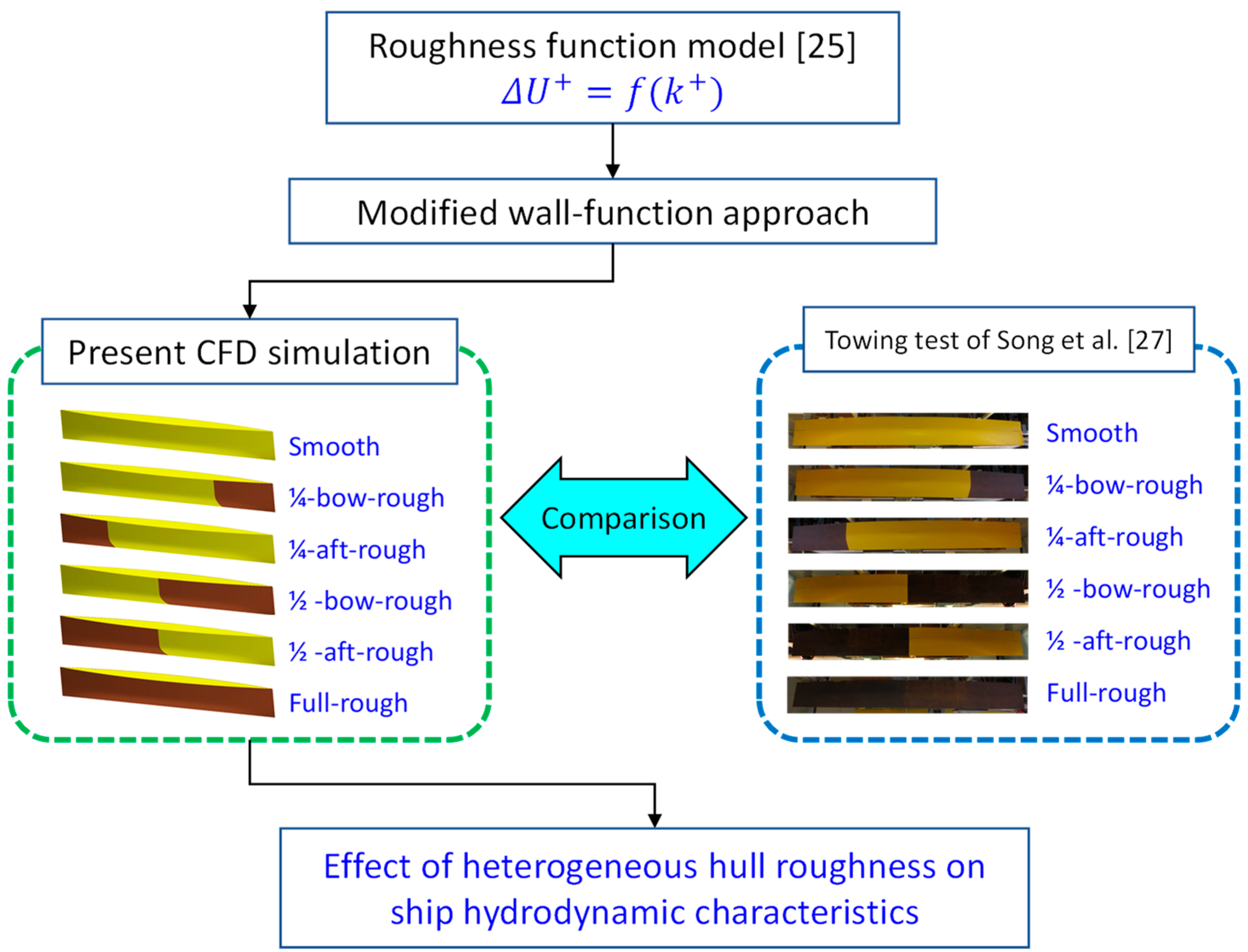
2.1. Approach
2.2. Numerical Modelling
2.2.1. Mathematical Formulations
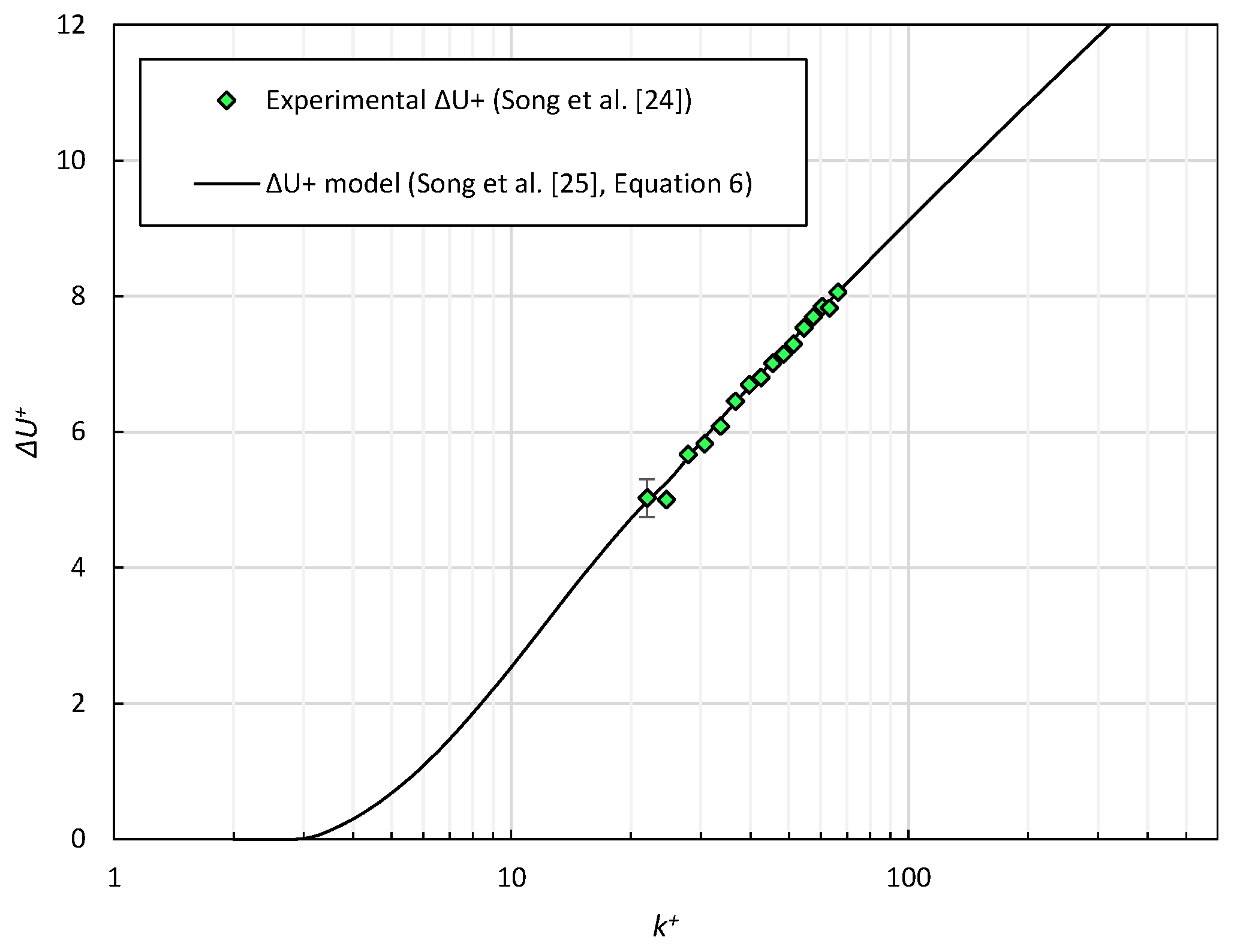
2.2.2. Modified Wall-Function Approach
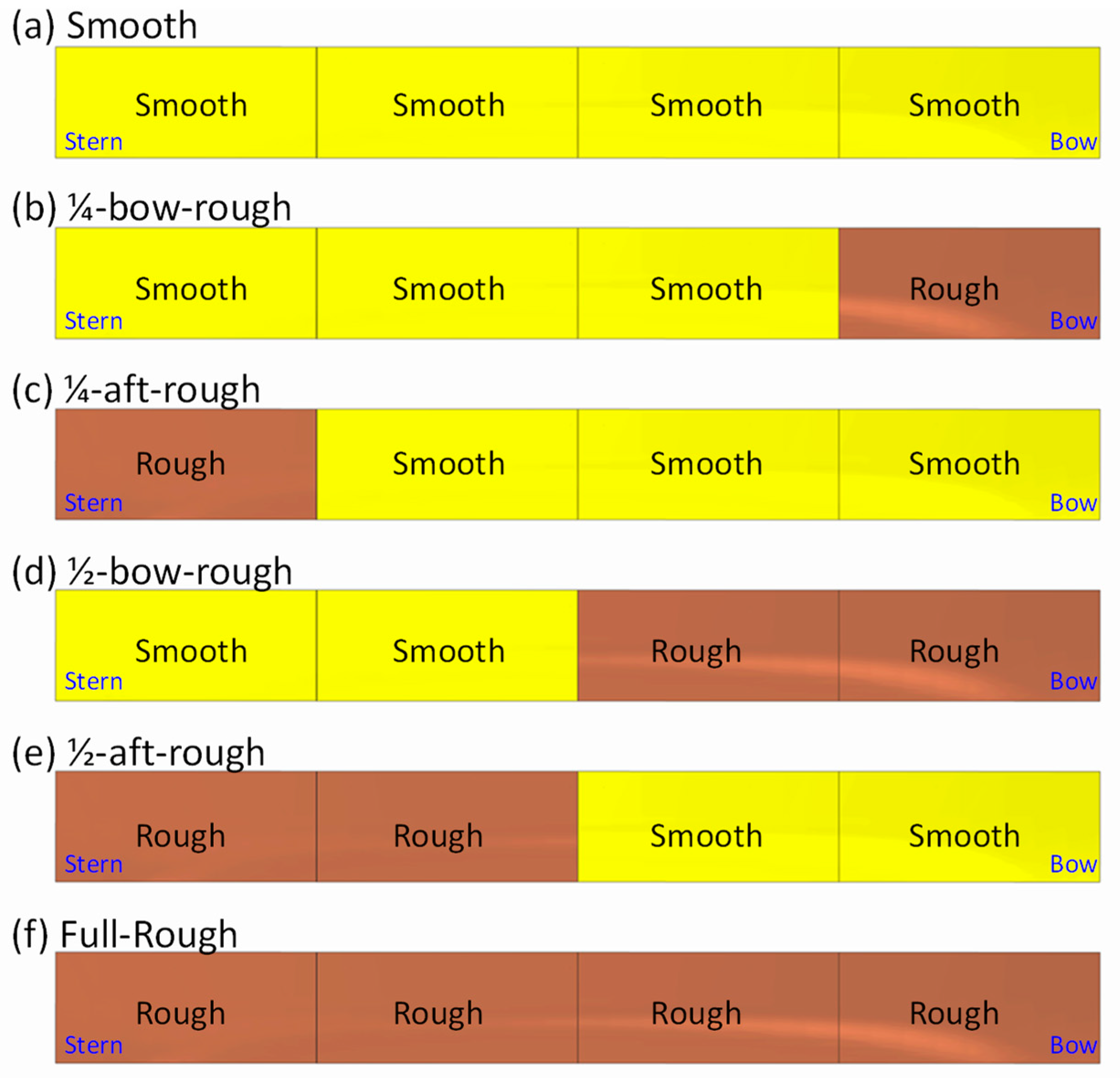
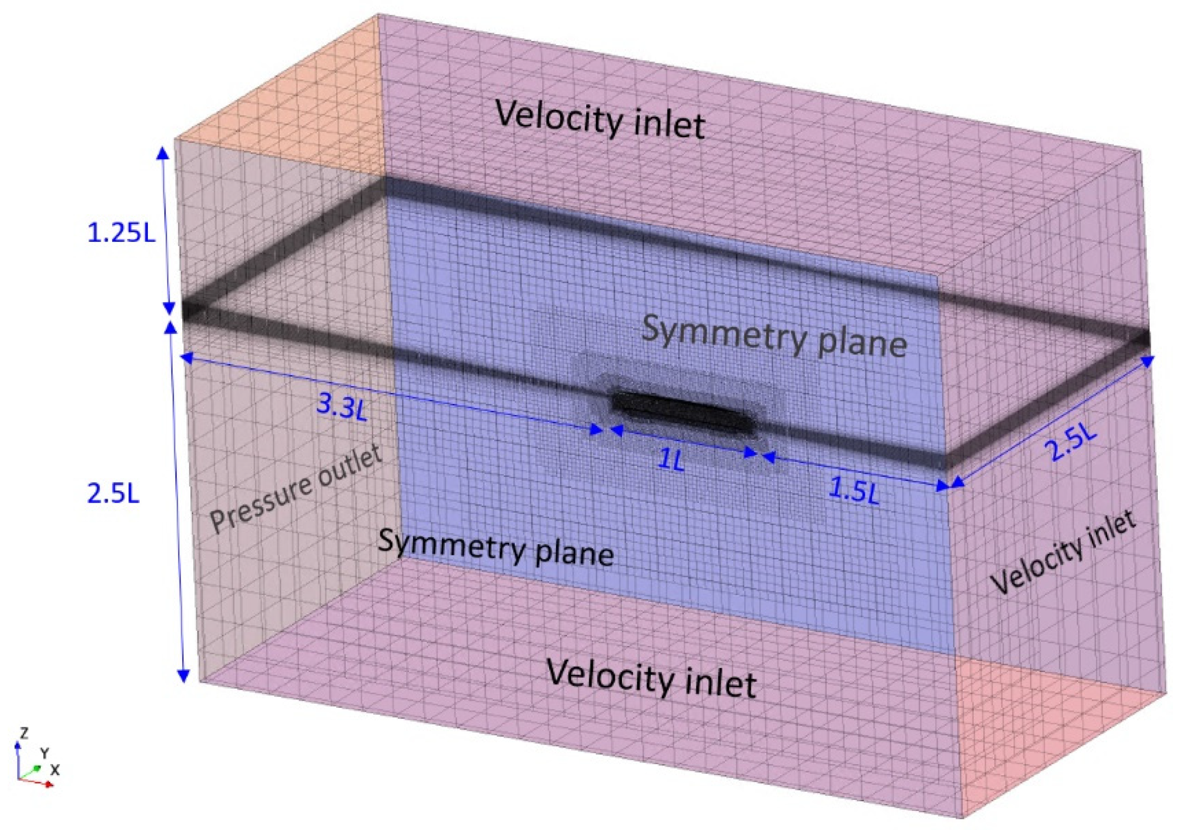
2.2.3. Geometry and Boundary Conditions
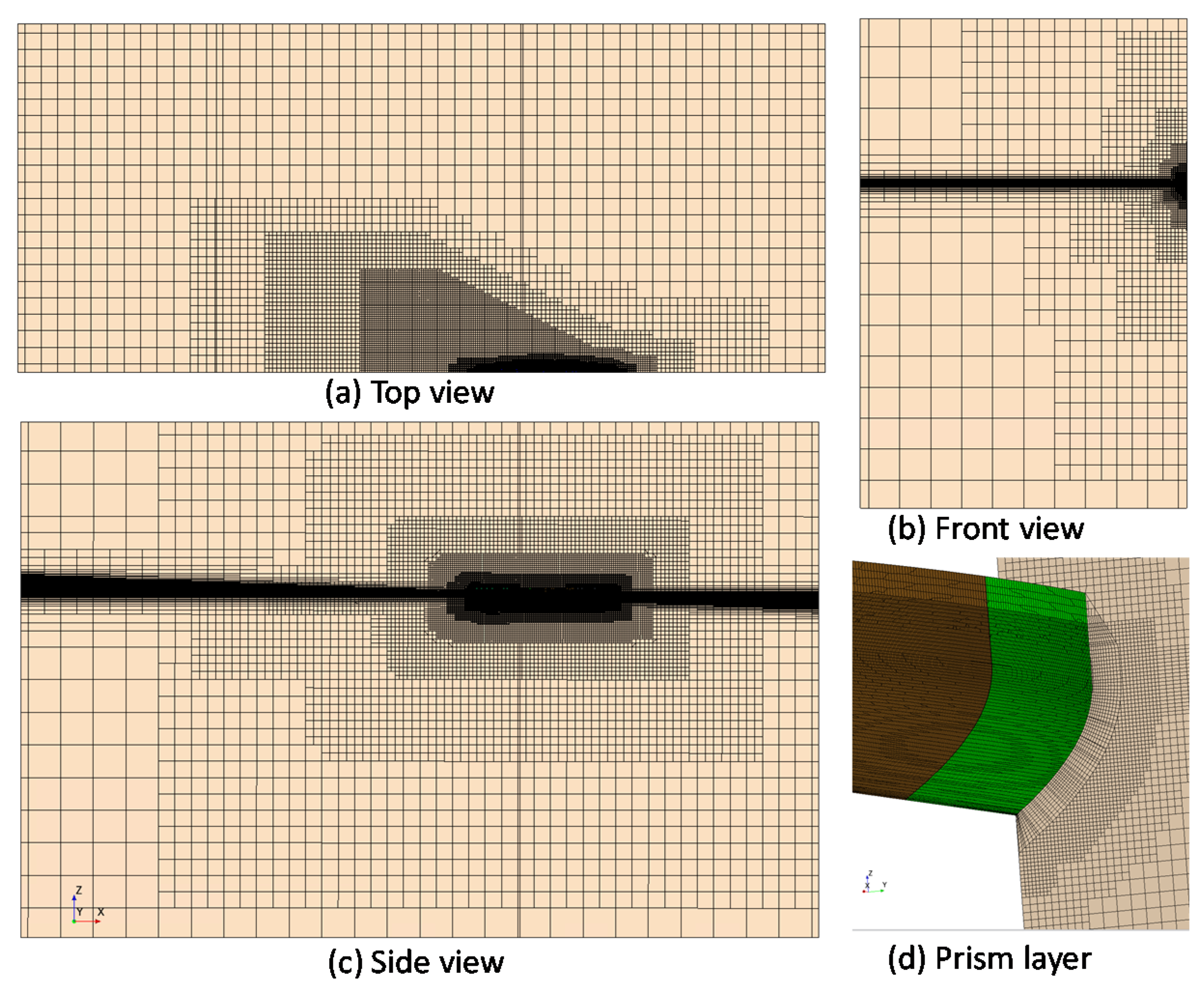
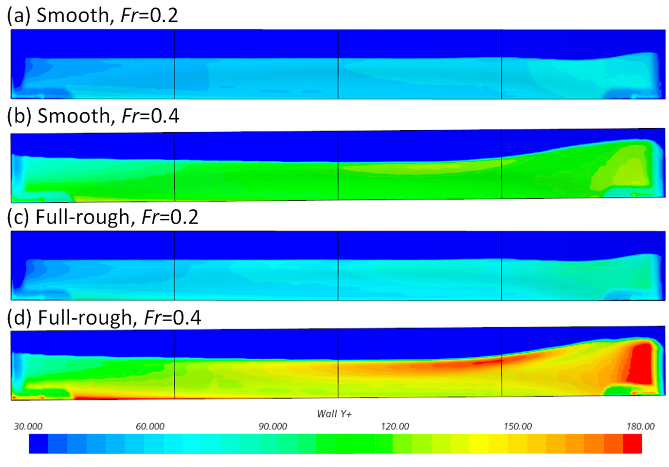
2.2.4. Mesh Generation
3. Results
3.1. Verification Study
3.2. Effect of Heterogeneous Roughness on Ship Resistance
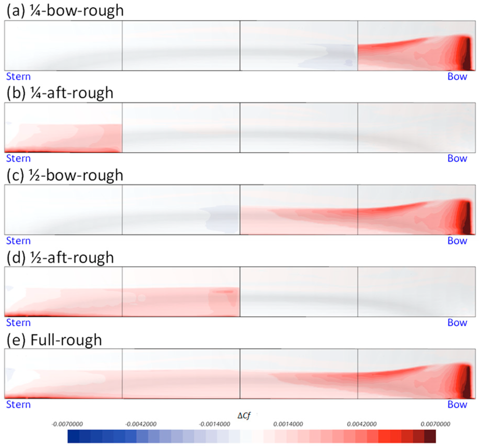
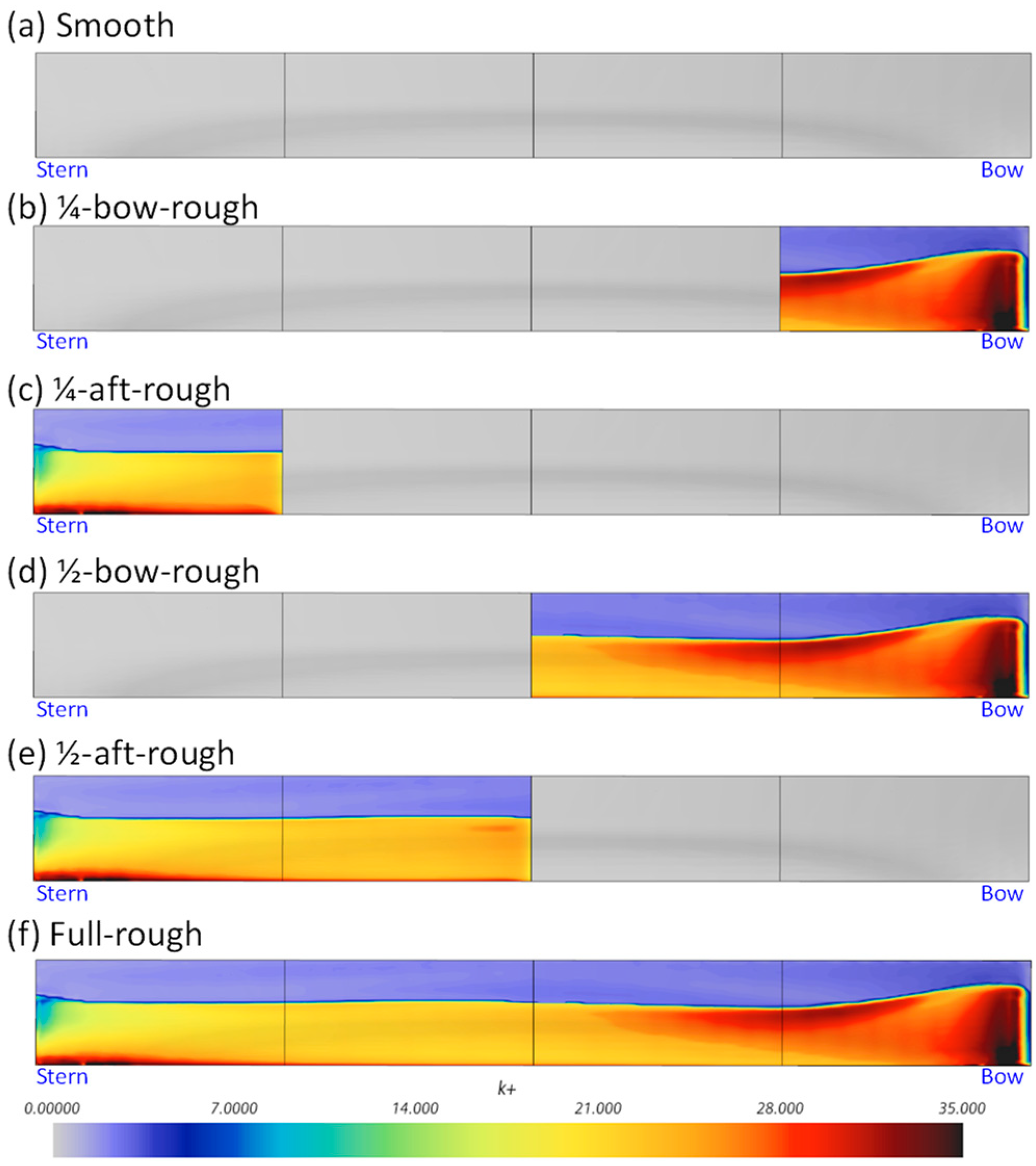
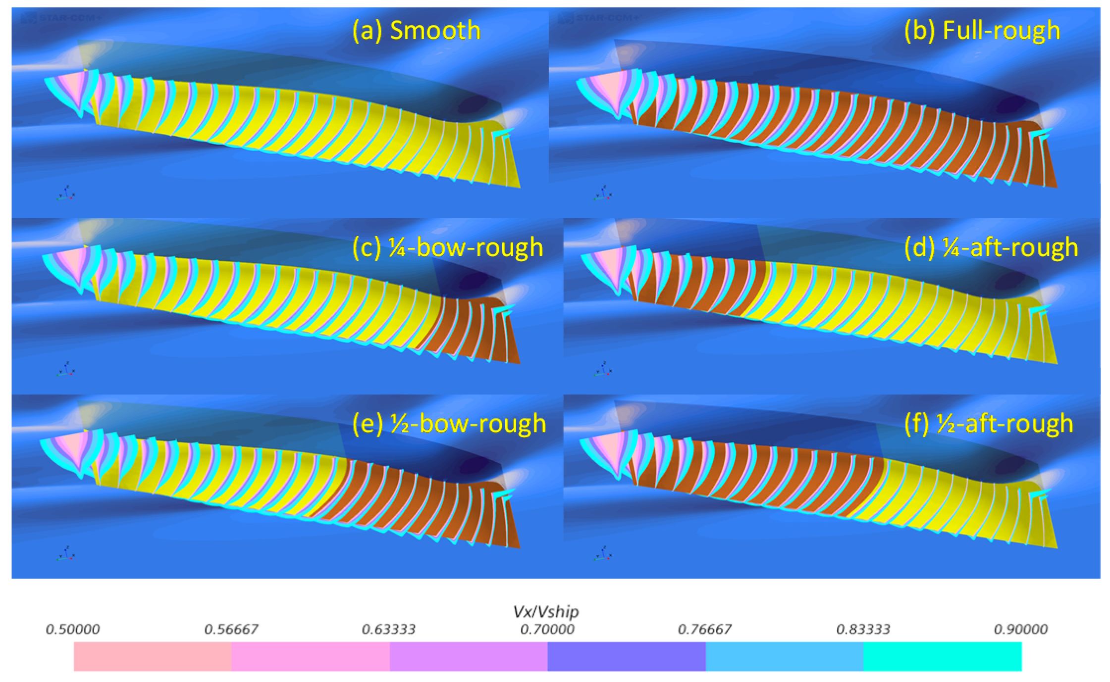
3.3. Rationale behind the Effect of Heterogeneous Roughness
4. Concluding Remarks
Author Contributions
Funding
Institutional Review Board Statement
Informed Consent Statement
Acknowledgments
Conflicts of Interest
Appendix A

| Smooth | 1/4-bow-rough | 1/4-aft-rough | |||||||
| Fr | CFD | EFD | %D | CFD | EFD | %D | CFD | EFD | %D |
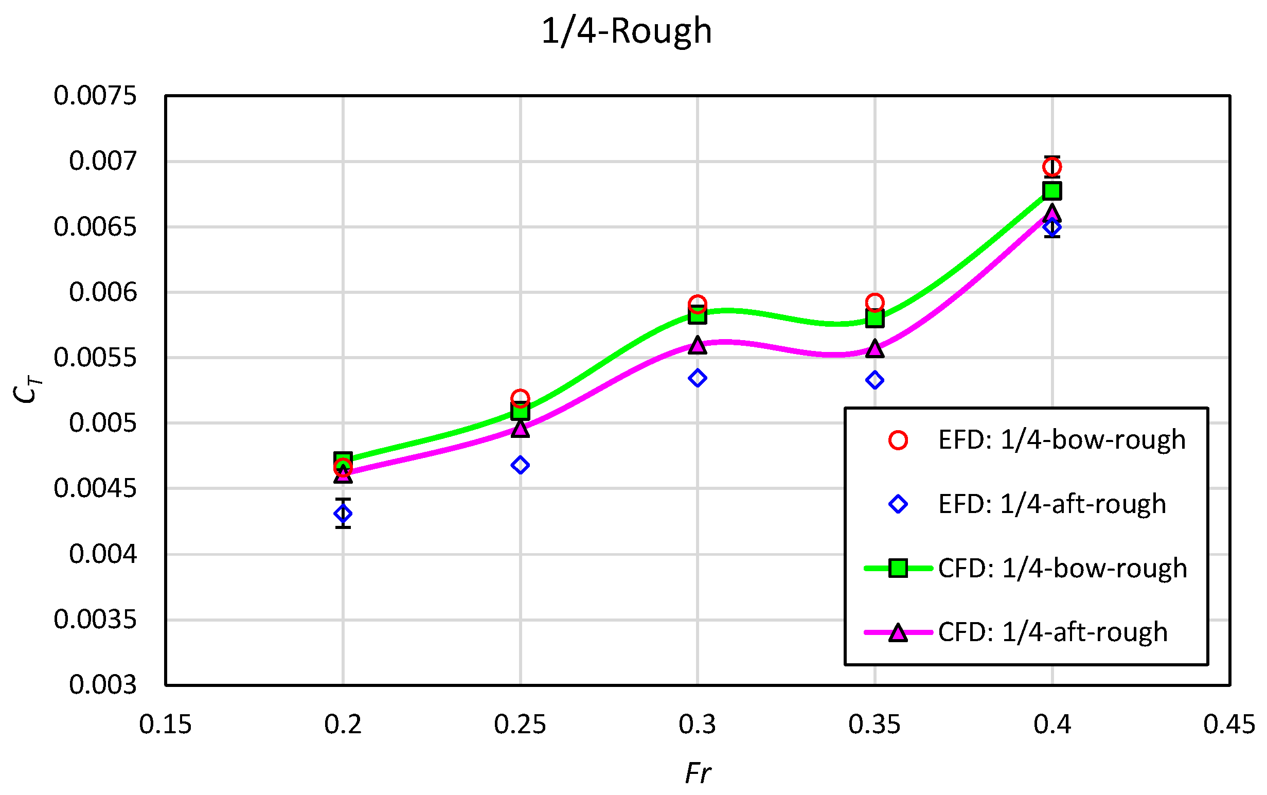
| 0.2 | 4.29 × 10⁻³ | 3.95 × 10⁻³ | −8.0% | 4.71 × 10⁻³ | 4.66 × 10⁻³ | −1.1% | 4.61 × 10⁻³ | 4.31 × 10⁻³ | −6.5% |
| 0.25 | 4.63 × 10⁻³ | 4.38 × 10⁻³ | −5.3% | 5.09 × 10⁻³ | 5.19 × 10⁻³ | 1.8% | 4.96 × 10⁻³ | 4.68 × 10⁻³ | −5.7% |
| 0.3 | 5.25 × 10⁻³ | 5.03 × 10⁻³ | −4.3% | 5.83 × 10⁻³ | 5.91 × 10⁻³ | 1.3% | 5.60 × 10⁻³ | 5.35 × 10⁻³ | −4.5% |
| 0.35 | 5.17 × 10⁻³ | 4.95 × 10⁻³ | −4.2% | 5.80 × 10⁻³ | 5.92 × 10⁻³ | 2.0% | 5.58 × 10⁻³ | 5.33 × 10⁻³ | −4.4% |
| 0.4 | 6.16 × 10⁻³ | 6.08 × 10⁻³ | −1.4% | 6.77 × 10⁻³ | 6.96 × 10⁻³ | 2.7% | 6.61 × 10⁻³ | 6.50 × 10⁻³ | −1.7% |
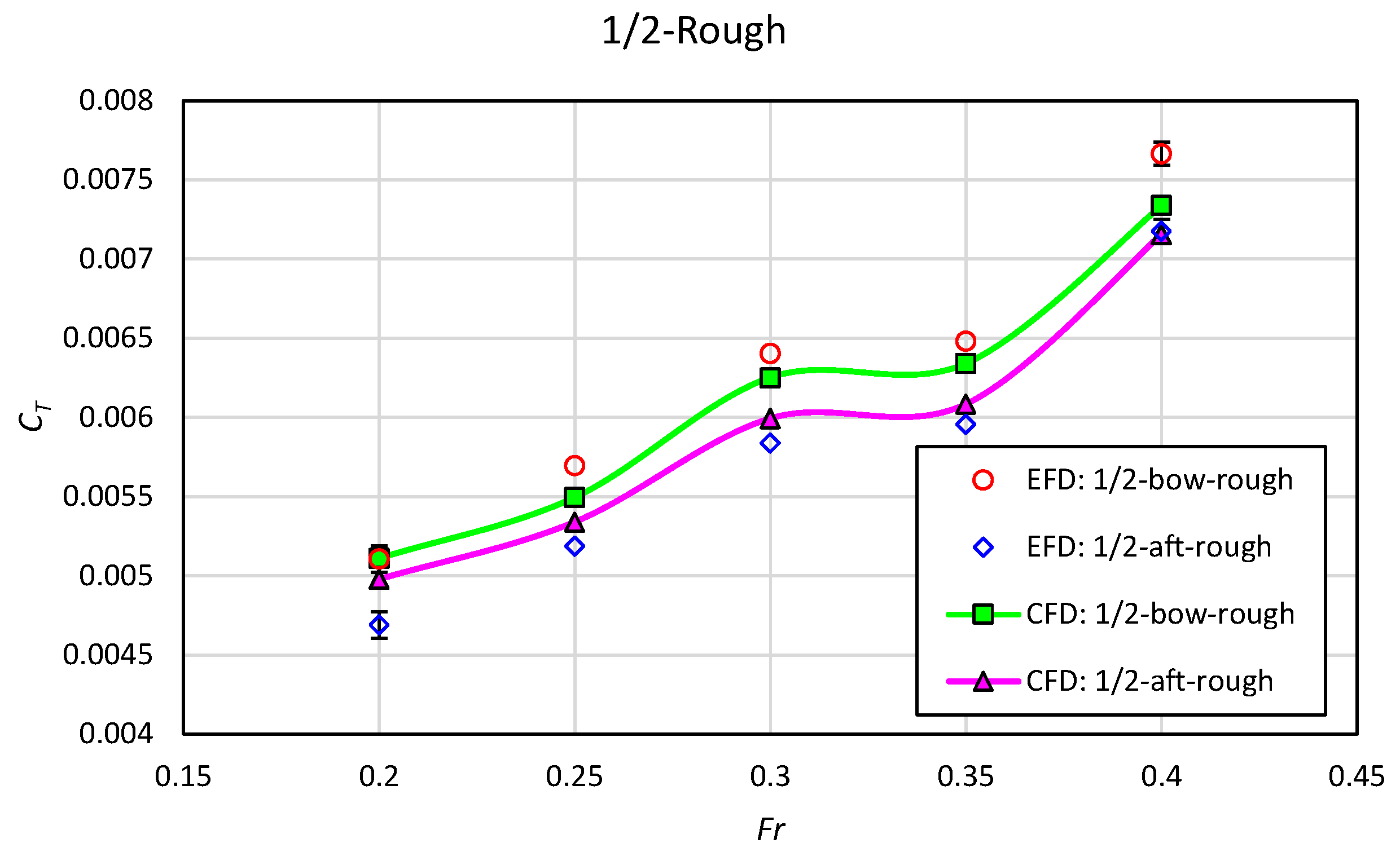
| 1/2-bow-rough | 1/2-aft-rough | Full-rough | |||||||
| Fr | CFD | EFD | %D | CFD | EFD | %D | CFD | EFD | %D |
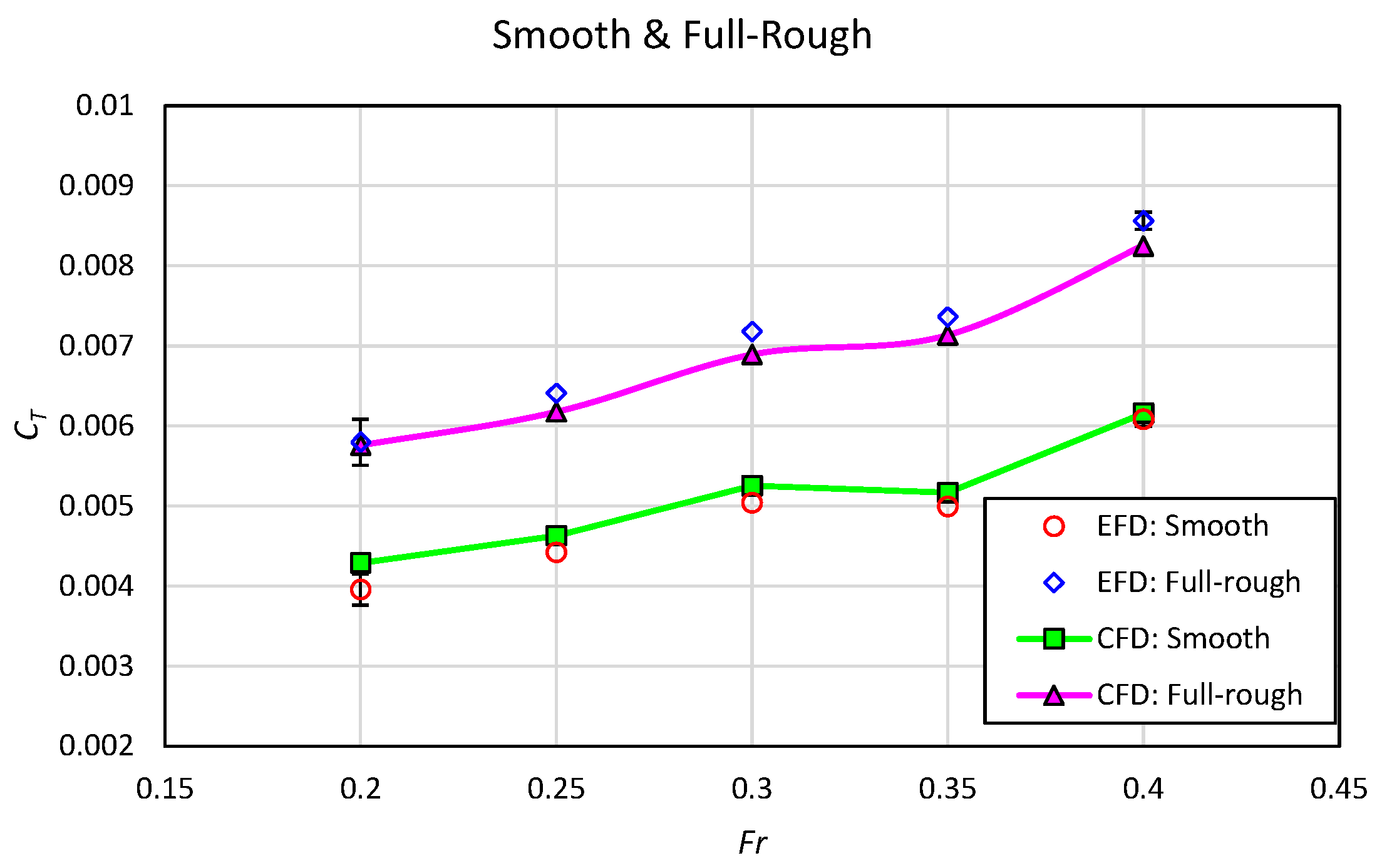
| 0.2 | 5.11 × 10⁻³ | 5.11 × 10⁻³ | −0.1% | 4.98 × 10⁻³ | 4.69 × 10⁻³ | −5.8% | 5.76 × 10⁻³ | 5.81 × 10⁻³ | 0.9% |
| 0.25 | 5.50 × 10⁻³ | 5.70 × 10⁻³ | 3.6% | 5.34 × 10⁻³ | 5.19 × 10⁻³ | −2.8% | 6.18 × 10⁻³ | 6.40 × 10⁻³ | 3.6% |
| 0.3 | 6.25 × 10⁻³ | 6.40 × 10⁻³ | 2.4% | 5.99 × 10⁻³ | 5.84 × 10⁻³ | −2.6% | 6.89 × 10⁻³ | 7.20 × 10⁻³ | 4.5% |
| 0.35 | 6.34 × 10⁻³ | 6.48 × 10⁻³ | 2.2% | 6.08 × 10⁻³ | 5.96 × 10⁻³ | −2.1% | 7.13 × 10⁻³ | 7.38 × 10⁻³ | 3.4% |
| 0.4 | 7.34 × 10⁻³ | 7.66 × 10⁻³ | 4.4% | 7.15 × 10⁻³ | 7.18 × 10⁻³ | 0.3% | 8.25 × 10⁻³ | 8.58 × 10⁻³ | 4.0% |
References
- Townsin, R.L. The ship hull fouling penalty. Biofouling 2003, 19, 9–15. [Google Scholar] [CrossRef]
- Tezdogan, T.; Demirel, Y.K. An overview of marine corrosion protection with a focus on cathodic protection and coatings. Brodogradnja 2014, 65, 49–59. [Google Scholar]
- Granville, P.S. The frictional resistance and turbulent boundary layer of rough surfaces. J. Ship Res. 1958, 2, 52–74. [Google Scholar] [CrossRef]
- Granville, P.S. Similarity-Law Characterization Methods for Arbitrary Hydrodynamic Roughnesses; Bethesda: Rockville, MD, USA, 1978. [Google Scholar]
- Schultz, M.P. The relationship between frictional resistance and roughness for surfaces smoothed by sanding. J. Fluids Eng. 2002, 124, 492–499. [Google Scholar] [CrossRef]
- Schultz, M.P. Frictional resistance of antifouling coating systems. J. Fluids Eng. 2004, 126, 1039–1047. [Google Scholar] [CrossRef] [Green Version]
- Schultz, M.P.; Flack, K.A. The rough-wall turbulent boundary layer from the hydraulically smooth to the fully rough regime. J. Fluid Mech. 2007, 580, 381–405. [Google Scholar] [CrossRef] [Green Version]
- Flack, K.A.; Schultz, M.P. Review of hydraulic roughness scales in the fully rough regime. J. Fluids Eng. 2010, 132, 041203. [Google Scholar] [CrossRef] [Green Version]
- Schultz, M.P.; Bendick, J.A.; Holm, E.R.; Hertel, W.H. Economic impact of biofouling on a naval surface ship. Biofouling 2011, 27, 87–98. [Google Scholar] [CrossRef]
- Oliveira, D.; Larsson, A.I.; Granhag, L. Effect of ship hull form on the resistance penalty from biofouling. Biofouling 2018, 34, 262–272. [Google Scholar] [CrossRef] [Green Version]
- Atlar, M.; Yeginbayeva, I.A.; Turkmen, S.; Demirel, Y.K.; Carchen, A.; Marino, A.; Williams, D. A rational approach to predicting the effect of fouling control systems on “in-service” ship performance. GMO J. Ship Mar. Technol. 2018, 24, 5–36. [Google Scholar]
- Cella, U.; Cucinotta, F.; Sfravara, F. Sail plan parametric CAD model for an A-class catamaran numerical optimization procedure using open source tools. In Proceedings of the 16th Asian Congress of Fluid Mechanics, Bangalore, India, 13–17 December 2019; pp. 547–554. [Google Scholar]
- Cirello, A.; Cucinotta, F.; Ingrassia, T.; Nigrelli, V.; Sfravara, F. Fluid–structure interaction of downwind sails: A new computational method. J. Mar. Sci. Technol. 2019, 24, 86–97. [Google Scholar] [CrossRef]
- Stern, F.; Wang, Z.; Yang, J.; Sadat-Hosseini, H.; Mousaviraad, M.; Bhushan, S.; Diez, M.; Sung-Hwan, Y.; Wu, P.-C.; Yeon, S.M.; et al. Recent progress in CFD for naval architecture and ocean engineering. J. Hydrodyn. 2015, 27, 1–23. [Google Scholar] [CrossRef]
- Wang, J.; Wan, D. Application progress of computational fluid dynamic techniques for complex viscous flows in ship and ocean engineering. J. Mar. Sci. Appl. 2020, 19, 1–16. [Google Scholar] [CrossRef]
- Demirel, Y.K.; Turan, O.; Incecik, A. Predicting the effect of biofouling on ship resistance using CFD. Appl. Ocean Res. 2017, 62, 100–118. [Google Scholar] [CrossRef] [Green Version]
- Song, S.; Demirel, Y.K.; Atlar, M. An investigation into the effect of biofouling on the ship hydrodynamic characteristics using CFD. Ocean Eng. 2019, 175, 122–137. [Google Scholar] [CrossRef] [Green Version]
- Song, S.; Demirel, Y.K.; Muscat-Fenech, C.D.M.; Tezdogan, T.; Atlar, M. Fouling effect on the resistance of different ship types. Ocean Eng. 2020, 216, 107736. [Google Scholar] [CrossRef]
- Song, S.; Demirel, Y.K.; Atlar, M. Propeller performance penalty of biofouling: Computational fluid dynamics prediction. J. Offshore Mech. Arct. Eng. 2020, 142, 1–22. [Google Scholar] [CrossRef]
- Farkas, A.; Degiuli, N.; Martić, I. The impact of biofouling on the propeller performance. Ocean Eng. 2021, 219, 108376. [Google Scholar] [CrossRef]
- Song, S.; Demirel, Y.K.; Atlar, M. Penalty of hull and propeller fouling on ship self-propulsion performance. Appl. Ocean Res. 2020, 94, 102006. [Google Scholar] [CrossRef]
- Farkas, A.; Song, S.; Degiuli, N.; Martić, I.; Demirel, Y.K. Impact of biofilm on the ship propulsion characteristics and the speed reduction. Ocean Eng. 2020, 199, 107033. [Google Scholar] [CrossRef]
- Song, S.; Demirel, Y.K.; Atlar, M.; Shi, W. Prediction of the fouling penalty on the tidal turbine performance and development of its mitigation measures. Appl. Energy 2020, 276, 115498. [Google Scholar] [CrossRef]
- Song, S.; Dai, S.; Demirel, Y.K.; Atlar, M.; Day, S.; Turan, O. Experimental and theoretical study of the effect of hull roughness on ship resistance. J. Ship Res. 2020, 1–10. [Google Scholar] [CrossRef]
- Song, S.; Demirel, Y.K.; Atlar, M.; Dai, S.; Day, S.; Turan, O. Validation of the CFD approach for modelling roughness effect on ship resistance. Ocean Eng. 2020, 200, 107029. [Google Scholar] [CrossRef] [Green Version]
- Demirel, Y.K.; Uzun, D.; Zhang, Y.; Fang, H.-C.; Day, A.H.; Turan, O. Effect of barnacle fouling on ship resistance and powering. Biofouling 2017, 33, 819–834. [Google Scholar] [CrossRef] [Green Version]
- Song, S.; Ravenna, R.; Dai, S.; De Marco Muscat-Fenech, C.; Tani, G.; Demirel, Y.K.; Atlar, M.; Day, S.; Incecik, A. Ex-perimental investigation on the effect of heterogeneous hull roughness on ship resistance. Ocean Eng. 2021, in press. [Google Scholar] [CrossRef]
- Östman, A.; Koushan, K.; Savio, L. Study on additional ship resistance due to roughness using CFD. In Proceedings of the 4th Hull Performance & Insight Conference (HullPIC’19), Gubbio, Italy, 6–8 May 2019. [Google Scholar]
- Vargas, A.; Shan, H.; Holm, E. Using CFD to predict ship resistance due to biofouling, and plan hull maintenance. In Proceedings of the 4th Hull Performance & Insight Conference (HullPIC’19), Gubbio, Italy, 6–8 May 2019. [Google Scholar]
- Menter, F.R. Two-equation eddy-viscosity turbulence models for engineering applications. AIAA J. 1994, 32, 1598–1605. [Google Scholar] [CrossRef] [Green Version]
- Dogrul, A.; Song, S.; Demirel, Y.K. Scale effect on ship resistance components and form factor. Ocean Eng. 2020, 209, 107428. [Google Scholar] [CrossRef]
- Siemens. STAR-CCM+, User Guide, Version 13.06.
- Celik, I.B.; Ghia, U.; Roache, P.J.; Freitas, C.J.; Coleman, H.; Raad, P.E. Procedure for estimation and reporting of uncertainty due to discretization in CFD applications. J. Fluids Eng. 2008, 130, 078001. [Google Scholar] [CrossRef] [Green Version]


| Length | (m) | 3.00 |
| Beam at waterline | (m) | 0.30 |
| Draft | (m) | 0.1875 |
| Beam/draft ratio | 1.6 | |
| Total wetted surface area | (m2) | 1.3383 |
| Wetted surface area of first quarter | (m2) | 0.3066 |
| Wetted surface area of first half | (m2) | 0.6691 |
| Displacement | (m3) | 0.0750 |
| Block coefficient | 0.4444 | |
| Towing speed | (m/s) | 1.08–2.17 |
| Froude number | 0.2–0.4 | |
| Reynolds number | 2.6–5.3 × 10⁶ | |
| Water temperature | (°C) | 12 |
| Spatial Convergence | No.Cells | (s) | ||
| Coarse | 414,173 | 0.01 | 5.292 × 10⁻³ | |
| Medium | 776,227 | 0.01 | 5.273 × 10⁻³ | |
| Fine | 1,587,310 | 0.01 | 5.267 × 10⁻³ | |
| (Fine) | 0.053% | |||
| Temporal Convergence | No.Cells | (s) | ||
| Coarse | 1,587,310 | 0.04 | 5.169 × 10⁻³ | |
| Medium | 1,587,310 | 0.02 | 5.258 × 10⁻³ | |
| Fine | 1,587,310 | 0.01 | 5.267 × 10⁻³ | |
| (Fine) | 0.022% | |||
| 0.057% |
Publisher’s Note: MDPI stays neutral with regard to jurisdictional claims in published maps and institutional affiliations. |
© 2021 by the authors. Licensee MDPI, Basel, Switzerland. This article is an open access article distributed under the terms and conditions of the Creative Commons Attribution (CC BY) license (http://creativecommons.org/licenses/by/4.0/).
Share and Cite
Song, S.; Demirel, Y.K.; De Marco Muscat-Fenech, C.; Sant, T.; Villa, D.; Tezdogan, T.; Incecik, A. Investigating the Effect of Heterogeneous Hull Roughness on Ship Resistance Using CFD. J. Mar. Sci. Eng. 2021, 9, 202. https://doi.org/10.3390/jmse9020202
Song S, Demirel YK, De Marco Muscat-Fenech C, Sant T, Villa D, Tezdogan T, Incecik A. Investigating the Effect of Heterogeneous Hull Roughness on Ship Resistance Using CFD. Journal of Marine Science and Engineering. 2021; 9(2):202. https://doi.org/10.3390/jmse9020202
Chicago/Turabian StyleSong, Soonseok, Yigit Kemal Demirel, Claire De Marco Muscat-Fenech, Tonio Sant, Diego Villa, Tahsin Tezdogan, and Atilla Incecik. 2021. "Investigating the Effect of Heterogeneous Hull Roughness on Ship Resistance Using CFD" Journal of Marine Science and Engineering 9, no. 2: 202. https://doi.org/10.3390/jmse9020202