Comparison of Macro-Scale Porosity Implementations for CFD Modelling of Wave Interaction with Thin Porous Structures

Abstract

Computational fluid dynamics (CFD) modelling of wave interaction with thin perforated structures is of interest in a range of engineering applications. When large-scale effects such as forces and the overall flow behaviour are of interest, a microstructural resolution of the perforated geometry can be excessive or prohibitive in terms of computational cost. More efficiently, a thin porous structure can be represented by its macro-scale effects by means of a quadratic momentum source or pressure-drop respectively. In the context of regular wave interaction with thin porous structures and within an incompressible, two-phase Navier–Stokes and volume-of-fluid framework (based on interFoam of OpenFOAM^®), this work investigates porosity representation as a porous surface with a pressure-jump condition and as volumetric isotropic and anisotropic porous media. Potential differences between these three types of macro-scale porosity implementations are assessed in terms of qualitative flow visualizations, velocity profiles along the water column, the wave elevation near the structures and the horizontal force on the structures. The comparison shows that all three types of implementation are capable of reproducing large-scale effects of the wave-structure interaction and that the differences between all obtained results are relatively small. It was found that the isotropic porous media implementation is numerically the most stable and requires the shortest computation times. The pressure-jump implementation requires the smallest time steps for stability and thus the longest computation times. This is likely due to the spurious local velocities at the air-water interface as a result of the volume-of-fluid interface capturing method combined with interFoam’s segregated pressure-velocity coupling algorithm. This paper provides useful insights and recommendations for effective macro-scale modelling of thin porous structures.

1. Introduction

Fluid interaction with thin perforated structures is of interest in a range of contexts. Applications in marine engineering include current and wave interaction with aquaculture containers [1,2] and breakwaters [3,4]. Another more general application is in tuned liquid dampers with baffles for building motion attenuation [5,6,7]. Thus, there is significant interest in the challenge of simulating the effect of these thin porous structures using computational fluid dynamics (CFD). Full geometric resolution of the porous microstructure [8,9] is unlikely to be computationally feasible for large scale structures. When large-scale effects such as global forces and the overall fluid-flow behaviour are of the main interest, it is useful to represent a perforated structure by its macro-scale effects. Instead of resolving the microstructural geometry explicitly, the effect of the structure on the fluid can be applied as a porous pressure-drop and momentum source term respectively. This approach is less computationally demanding than microstructural CFD modelling [4,10,11], which requires a large number of mesh cells and also makes less restrictive assumptions compared to models based on potential-flow theory [12,13,14].

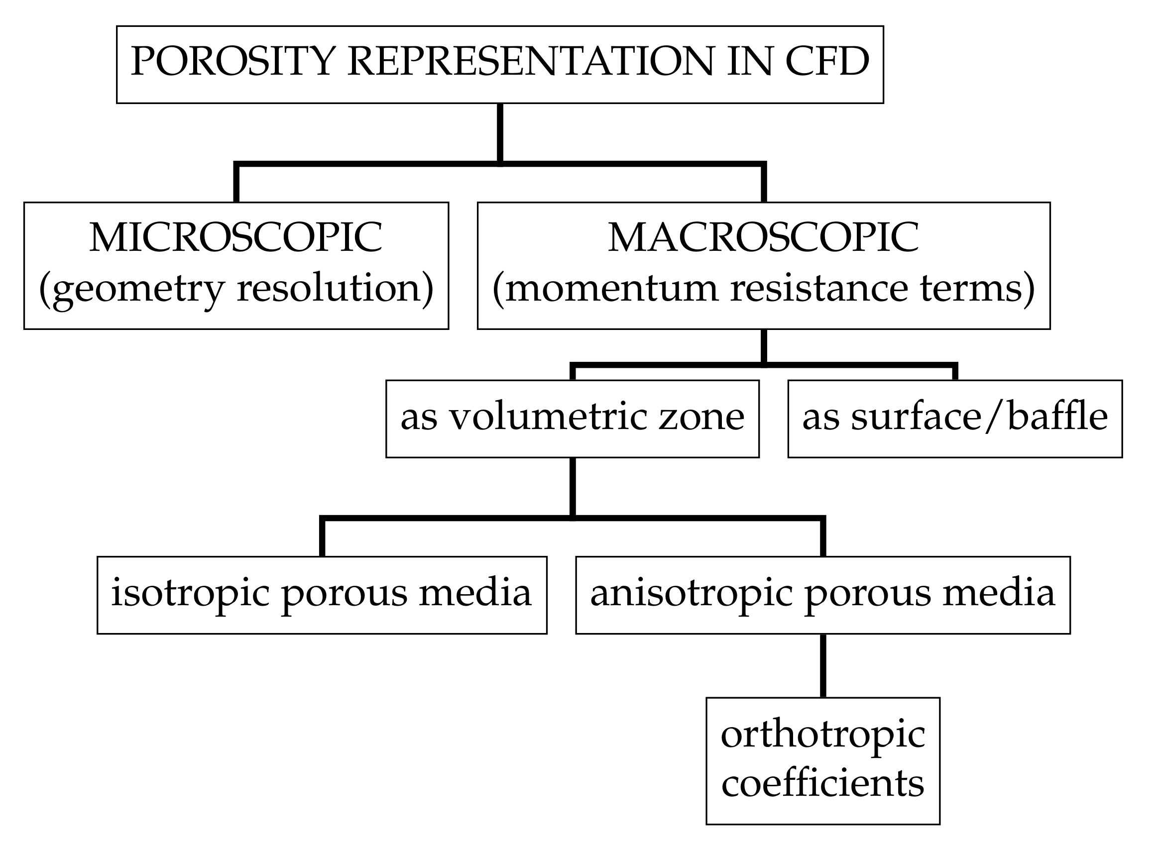
This paper presents an assessment of different macro-scale methods for the representation of thin perforated structures exposed to regular waves. The investigated options are the implementation as a two-dimensional (2D) surface with zero thickness and as volumetric three-dimensional (3D) porous media. The porous-media approach can accommodate isotropic or anisotropic material characteristics, where we can distinguish orthotropic characteristics (in which the porosity has separate values in three perpendicular rotationally symmetric axes) as a sub-category of the latter. Figure 1 outlines the main types of porosity representation in CFD modelling investigated here. While the porous-media approach can be used for both thin and volumetric structures, the porous surface or baffle implementation is only valid for thin structures. 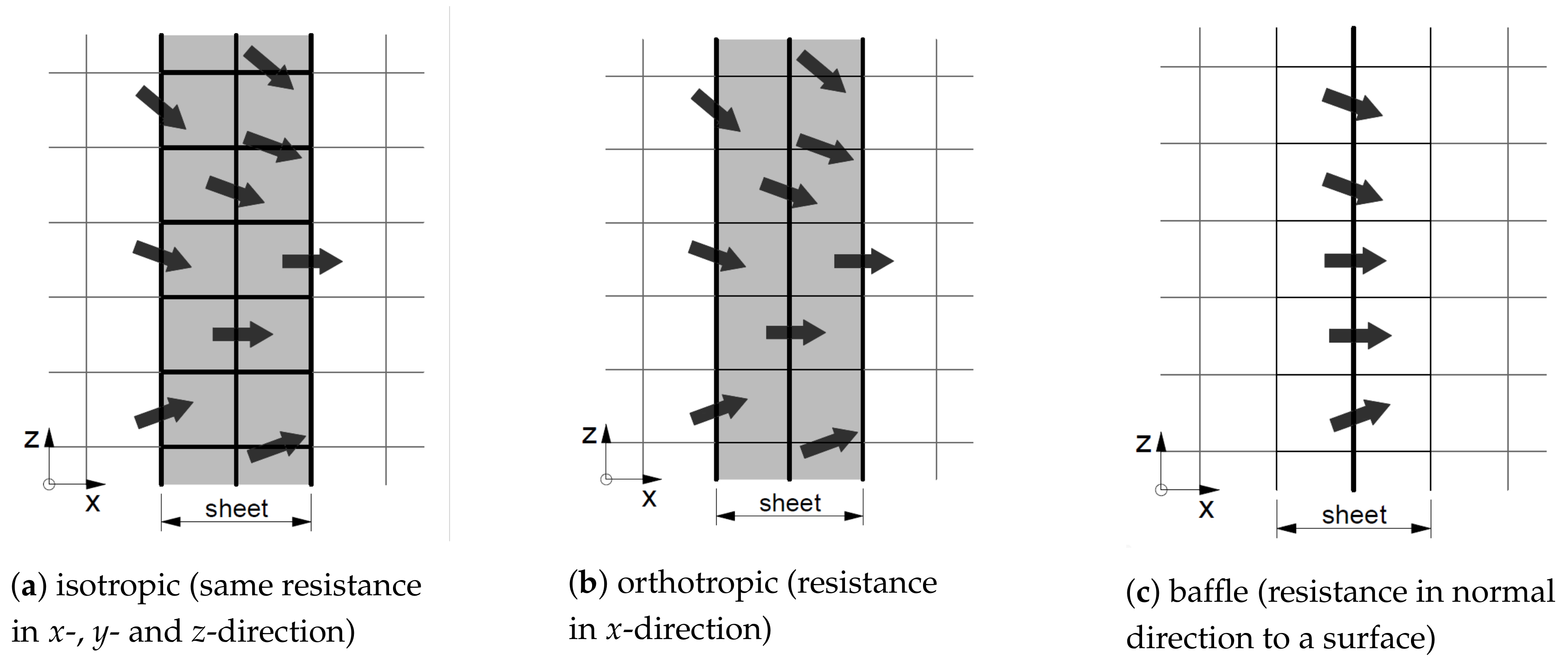Figure 2 shows schematics of the main types of macro-scale porosity representation investigated. In the sketches, the arrows outline velocity vectors close to the porous barrier and the bold lines along the cell faces indicate the components of the velocity that are subject to a pressure-drop.

The representation as a porous surface, often referred to as a porous baffle, uses a pressure-jump condition where a resistance source is applied to the Navier–Stokes momentum equation at the cell faces of a geometrically defined surface. The resistance source and pressure-jump respectively are commonly specified as a function of the velocity component normal to the surface. This approach is commonly used for structures where the thickness can be assumed to be negligibly small, such as membranes, fans, actuator disks, perforated baffles or fish nets. Examples of its use to represent membranes include studies on separation processes by Li and Cheng [15] or examinations of the flow field through perforated tiles in data centers by Arghode and Joshi [16]. For fans, the baffle-implementation has been used by Chacko et al. [17] to improve radiator efficiency by air flow optimization, by van der Spuy and von Backström [18] and Sumara and Šochman [19] to represent fans in air-cooled condensers. In the form of a perforated baffle, it has been used to simulate contact tanks for water treatment by Kizilaslan et al. [20] or in refrigeration cabinets by Wang et al. [21]. The same pressure-jump principle has also been used in the form of actuator disks for wind turbine rotors [22], tidal turbines [23], ship propellers [24] and helicopter rotors [25,26]. As a marine engineering application similar to the present case, Shim et al. [2] have used a porous baffle to model current flow through and around a cylindrical fish net cage. Most of the existing research described here has been performed for steady-state conditions and in single phase flow. Bakica et al. [24] investigated ship resistance with two phases, but the actuator-disk that represents the ship propeller was fully submerged in the water. Apart from applications to actuator disks [22,25,26] and for water treatment [20], steady-state solutions have been calculated in most previous examples.

Porosity representation as a volumetric porous zone, often referred to as porous media, is implemented as momentum resistance applied to the cell centres (in a cell-centered finite-volume framework) of a volumetrically defined geometric region. The porous media can be implemented with either isotropic or anisotropic characteristics and the resistance-source terms can be formulated by means of either scalar or tensor values respectively. It can furthermore be used with or without consideration of the reduced amount of fluid inside the volume as a result of the geometric blockage of the porous structure. Typically, for large volumetric structures such as dams or breakwaters, the reduced amount of fluid needs to be taken into account and the volume-averaged Navier–Stokes equations or volume-averaged Reynolds-averaged Navier–Stokes (VARANS) equations are used, which are formulated for the intrinsic velocity inside the porous structure. Higuera et al. [27], Lara et al. [28] and del Jesus et al. [29] have used porous-media VARANS-formulations with isotropic material characteristics for studies on fluid interaction with dams, cubical porous barriers and Brito et al. [30] and Hadadpour et al. [31] have used it for fluid interaction with vegetation. Chen and Christensen [1] used a volume-averaged Navier–Stokes formulation with anisotropic material characteristics for plane and circular fish nets. Using 2D models, they investigated current flow across a truncated plane with various angles of attack, wave interaction with bottom-fixed vertical sheets, whilst in a 3D model, they looked at current flow across a truncated fully submerged cylinder.

In previous work, we have used a volume-averaged Navier–Stokes formulation with isotropic material assumptions to model wave interaction with thin perforated sheets and cylinders in [32,33]. Qiao et al. [34] have used an identical method and achieved good agreement between CFD results and the same experimental results of wave interaction with vertical sheets. For other cases of thin porous structures, the Navier–Stokes or Reynolds-averaged Navier–Stokes (RANS) equations have previously been used inside and outside the porous structure neglecting the effects of a reduced fluid amount in the openings. This was done so with anisotropic material assumptions by Kyte [35] for the representation of a filter as part of a domestic ventilation waste heat recovery system and by Zhao et al. [36,37] for rigid plane fish nets. The anisotropic approach can also be used to direct the fluid flow in a certain way, as demonstrated for instance by Hafsteinsson [38] to model flow through a conical diffuser.

For all these implementations, the formulation of the pressure-drop resistance and its corresponding porosity coefficients are of key importance. For fluid flow across thin perforated structures, the flow regime is typically turbulent with high Reynolds numbers ($Re$); where turbulent drag forces dominate, transient losses have a minor effect on the flow and viscous forces can be considered to be negligible. In the context of fluid interaction with fish net cages, Shim et al. [2] used a drag force with a porosity coefficient obtained from experiments in combination with a baffle implementation.  Zhao et al. [36,37] have used both a viscous force and drag force with coefficients based on empirical formulations within a porous-media RANS implementation. With a porous-media VARANS-approach, Chen and Christensen [1] have applied both a drag and a transient resistance term. The drag coefficient was obtained from a Morison-type load-model that assumes a fish net being composed of cylindrical twines without knots. The transient coefficient was arguably set to 0.43 without further investigations and declared to be an inherited parameter from work on large volumetric dams by Jensen et al. [39].

The present work on thin structures with numerous circular perforations omits the viscous and transient pressure-drop terms and uses a drag term with a drag coefficient as a function of porosity. The use of this assumption in previous work demonstrated good agreement between CFD, potential-flow and experimental results for wave interaction with vertical sheets and cylinders [33]. The methodology is further explained in Section 3.1. This theoretical pressure-drop formulation avoids calibration procedures, in contrast to the approaches by Shim et al. [2] and Chen and Christensen [1]. The focus of the current work is the assessment of the different pressure-drop implementation approaches, as outlined in Figure 1. As part of the assessment, this work explores the use of a porous baffle for transient two-phase wave-structure interaction as a new application. It furthermore uses a porous-media approach with orthotropic material properties for two-phase wave interaction with a bottom-fixed cylinder. A 2D model of a thin perforated bottom-fixed sheet and a 3D model with a thin perforated bottom-fixed cylinder exposed to regular waves are simulated. The aim is to compare the different types of porosity implementations by means of flow visualizations, water velocity profiles, the mean flow behaviour in terms of wave gauge signals and the horizontal force on the structures. The outcome of this work can serve as a guide for CFD model setup for similar applications in a marine engineering context.

This paper is structured as follows. Firstly, a brief outline of the experiments conducted for model validation is given in Section 2. Then, the numerical method is explained in Section 3 and the specific model setup in Section 4. The results are presented in Section 5, showing the comparison between the investigated types of macro-scale porosity implementations. This is followed by a discussion in Section 6 and conclusions in Section 7.

2. Wave Flume Experiments

This work focuses on the comparison between CFD models with different types of porosity implementations, but experimental results are included for reference. For detailed information and photos of the experiments, we refer to [33,40,41], but relevant aspects of the setup are outlined in the following.

Wave tank tests to investigate wave interaction of thin perforated vertical sheets and cylinders were conducted at Dalian University of Technology, China, where the wave flume has a length of 60 m and is equipped with a piston wavemaker at one end and a sloped beach at the other end. The tests were performed with a water depth of $h=$ 1.0 m and two separate test-sections; one for a sheet with a width of 1 m and one for a cylinder with a width of 3 m. A range of geometrical parameters such as sheet thicknesses (3 mm $⩽d⩽$ 10 mm), hole separation distances (25 mm $⩽s⩽$ 100 mm), outer cylinder diameters (0.375 m $⩽D⩽$ 0.750 m) and porosities (0.1 $⩽n⩽$ 0.4) have been tested simultaneously under a range of regular and irregular wave conditions. The porosity, n, is defined as $n=\pi r_h^2/s^2$ (the ratio of void volume to total volume) for a regular rectangular grid of holes, where the hole centre spacing was kept constant with s = 25 mm and the perforation hole radius, $r_h$, was varied. On the top and bottom end of both structures, load cells were attached to measure the wave-induced horizontal load.

In this numerical work, only one combination of wave and geometrical parameters per structure has been investigated, since the validity of the theoretical pressure-drop model for other parameters has been demonstrated in previous work, [33]. All 2D models have been set up with a vertical bottom-fixed sheet with a thickness of d = 10 mm and all 3D models with a bottom-fixed cylinder with an outer diameter of D = 0.50 m and a thickness of d = 5 mm. Both structures had a porosity of n = 0.2. A single regular wave condition is used for all CFD models. The wave parameters used here are shown in

Table 1. Water depth, h, and wave parameters used in the present study (input and target parameters).

h [m]		T [s]	$\mathit{\lambda }$ [m]	H [m]	A [m]	$\mathit{kh}$ [-]	$\mathit{kA}$ [-]	${\mathit{c}}_{\mathit{g}}$ [m/s]
1.00		2.1	5.58	0.1775	0.08875	1.13	0.10	1.96

, where T is the wave period, $\lambda$ is the wavelength, H is the wave height, $c_g$ is the group velocity, $kh$ is the non-dimensional wave number (with h as the water depth and k as the wave number) and $kA$ is the wave steepness (with A as the wave amplitude).

3. Numerical Method

This work uses a theoretical pressure-drop formulation as a momentum source in all present CFD models. Its formulation is based on the specific characteristics of oscillatory wave flow across thin sheets with numerous circular perforations.

3.1. Theoretical Pressure-Drop Formulation

The flow regime close to the perforated barrier is dominated by turbulence, as indicated by the large $Re$-numbers in this region. Viscous losses can thus be considered to have negligible effects [42]. Transient losses have a minor effect and tend to zero when the size of the perforations is small relative to the wavelength [43]. Consequently, viscous and transient losses are assumed to be zero in this work and the pressure drop, $\Delta p$, across the perforated barrier is specified as a drag term and formulated as

$$\Delta p=\frac{\rho C_f}{2}\mathit{U}\left|\mathit{U}\right|,$$

(1)

where $\rho$ is the fluid density, $C_f$ is a drag or porosity coefficient and $\mathit{U}$ is the fluid velocity averaged over the cell area, often referred to as Darcy velocity. The latter is related to the actual velocity in the porous media, $\mathit{u}$, by $\mathit{U}=\mathit{u}\ast n$.

This work uses a formulation by Molin [43] to define $C_f$:

$$C_f=\frac{1-n}{\delta n^2}.$$

(2)

$\delta$ is an empirically defined discharge coefficient, usually in the range of 0.4–0.5. For oscillatory flow, the discharge coefficient, $\delta$, and therefore $C_f$, vary with the Keulegan–Carpenter ($KC$) number, defined as

$$KC=\frac{u_{m}T}{L},$$

(3)

where $u_m$ is the amplitude of the oscillating flow velocity, T is the oscillation period and L is a characteristic length. For the present wave condition, the $KC$ number has been estimated for the small-scale flow across the structure to be $KC$ = 29.5 with $u_m$ as the horizontal velocity at the free surface, T as the wave period and L as the hole centre spacing of the cylinder perforations of s = 25 mm. The variation of the coefficient $C_f$ with $KC$ for slatted sheets has been investigated by Tait et al. [6] and Hamelin et al. [7]. They found that for $KC\gtrsim$ 15, the influence of $KC$ on $C_f$ decreases and $C_f$ tends to the value for steady flow. Therefore, the present work assumes the influence of $KC$ to be negligible and uses $\delta =0.5$. This value was found to have good agreement between experimental results and numerical results from both previous CFD modelling, [33], and from a potential-flow model by Mackay et al. [40].

3.2. Governing Equations

For the present work, the open source CFD code OpenFOAM^® (The OpenFOAM Foundation v5) [44] is used with its implementation of the incompressible, immiscible, two-phase Navier–Stokes equations and the volume-of-fluid (VOF) interface-capturing method with the multidimensional universal limiter for explicit solution (MULES) for boundedness preservation [45].

The Navier–Stokes mass conservation equation is written as

$$\nabla ·\mathit{U}=0.$$

(4)

The formulation of the momentum conservation equations differs depending on the type of porosity implementation. The pressure-drop application varies for the isotropic and orthotropic porous media and the porous baffle implementation, as outlined in Figure 2. In the case of a porous-baffle implementation, an internal pressure-jump condition is applied at the cell faces of a geometrically defined surface with zero thickness. This is outlined in Figure 2c. At the mesh cell faces of this surface, the pressure-drop as defined by (1) is applied to the Navier–Stokes momentum equation, which is then written as

$$\frac{\partial }{\partial t}\rho \mathit{U}+\nabla ·\rho \mathit{U}\mathit{U}=-\nabla p^{\ast }-\mathit{g}\mathit{X}\nabla ·\rho +\nabla ·({\mu }_{eff}\nabla \mathit{U})+\sigma \kappa \nabla \alpha -\Delta p,$$

(5)

where $\mathit{X}$ is the position vector in Cartesian coordinates, $\mathit{g}$ is the vector of gravitational acceleration and $p^{\ast }$ is the pseudo-dynamic pressure (used for numerical convenience instead of the actual dynamic pressure [46]). The term with the surface tension coefficient, $\sigma$, and the curvature of the interface, $\kappa$, represents surface tension effects. $\rho$ is the weighted averaged density, calculated as $\rho =\alpha {\rho }_w+(1-\alpha ){\rho }_a$, where ${\rho }_w$ is the water density, ${\rho }_a$ is the air density and $\alpha$ the phase-fraction. ${\mu }_{eff}$ is the effective dynamic viscosity and is calculated from the molecular viscosity, $\mu$, and the turbulent eddy viscosity, ${\mu }_{turb}$, as ${\mu }_{eff}=\mu +{\mu }_{turb}$. The eddy viscosity, ${\mu }_{turb}$, represents small-scale isotropic turbulent effects by means of a turbulence model. In the same way as for the density, the viscosity, $\mu$, in the momentum equation is the phase-weighted value calculated from the water and air viscosities, ${\mu }_w$ and ${\mu }_a$, as $\mu =\alpha {\mu }_w+(1-\alpha ){\mu }_a$. $\alpha$ is used to capture the interface as part of the VOF method and follows an advection equation, defined as

$$\frac{\partial \alpha }{\partial t}+\left(\nabla \mathit{U}\alpha +\nabla {\mathit{U}}_{\mathit{c}}(1-\alpha )\alpha \right)=0,$$

(6)

where ${\mathit{U}}_{\mathit{c}}$ is an artificial compression velocity as part of an interface compression term [47]. $\alpha =1$ corresponds to a mesh cell full of water, $\alpha =0$ to a cell full of air and cells with 0 $<\alpha <$ 1 are part of the free water surface.

When the pressure-drop is introduced by means of a volumetrically defined porous zone, the momentum source term is applied to the mesh cell centers (OpenFOAM^® uses a cell-centred finite-volume approach). For the models with porous media, OpenFOAM^® is used with modifications used in both the OlaFlow/IHFoam [48] and waves2Foam [39,49] libraries. These toolboxes provide solvers based on OpenFOAM^®’s standard solver for incompressible, immiscible two-phase flow with the VOF interface-capturing method interFoam and are tuned for free-surface waves and incorporate the use of porous-media modelling. Both use the volume-averaged Reynolds-averaged Navier–Stokes (VARANS) equations based on derivations following [50,51,52]. Their comprehensive derivation can be found in [27,39]. The resulting VARANS equations look the same as the mass conservation Equation (4), and the momentum Equation (5), but are formulated for the intrinsic velocity, $\mathit{U}/n$ (the mean velocity of the fluid inside the perforations), instead of $\mathit{U}$. This takes account of the geometric blockage effect mentioned above. Correspondingly, the pressure-drop formulation (1), and the VOF $\alpha$-Equation (6), are formulated with $\mathit{U}/n$. Inside the porous zone, the macro-scale effects of the porous barrier are applied by means of a momentum source term and with a reduced fluid amount. Outside the porous zone, the VARANS equations are equal to the standard RANS equations (i.e., n = 1). interFoam and the derived solvers of OlaFlow/IHFoam and waves2Foam use the transient PIMPLE algorithm (a combination of the SIMPLE and PISO algorithm) implemented to solve the pressure-velocity coupling in a segregated manner. Further information on those algorithms can, for instance, be found in [53].

The volumetric porous-media approach can be implemented with either isotropic or anisotropic material characteristics. In the isotropic case, the pressure-drop is applied as a single scalar quantity identical in all directions, outlined in Figure 2a. In the anisotropic case, the pressure-drop can vary in location and direction. This is often implemented in terms of orthotropic characteristics with three main directions (as a sub-type of anisotropic properties). For the case of a thin perforated sheet, this corresponds to a normal direction across the sheet and two in-plane directions, as outlined in Figure 2b, and this ideally reflects the reality of a sheet with holes cut in it (small resistance to flow in one direction, infinite in the perpendicular directions). The orthotropic porosity implementation is realized with the porosity coefficient, $C_f$, implemented as a tensor field, ${\mathit{C}}_{\mathit{f}}$. For the specific case of a thin perforated barrier, the pressure-drop is only applied in a normal direction across the sheet and therefore dependent on the flow velocity normal to it. An isotropic implementation can be realized either by using the same value for $C_f$ in all three main directions of the tensor field, ${\mathit{C}}_{\mathit{f}}$, or by directly using a scalar field for $C_f$. The implementation of ${\mathit{C}}_{\mathit{f}}$ as tensor field is the standard implementation in waves2Foam. In this work, the porosity solver of waves2Foam was modified for application to a porous cylinder where a transformation between the local cylindrical coordinate system (radial, tangential, vertical) and the global Cartesian coordinate system (x, y, z) has been introduced. The implementation of $C_f$ as scalar field is the standard implementation in OlaFlow/IHFoam which has been used without modifications.

3.3. Flow Scales and Turbulence-Free Modelling

In the present context of wave interaction with thin perforated sheets and cylinders, we make a distinction between two main flow scales, the large-scale flow around the structure and the small-scale flow across the sheet through the openings. Large-scale turbulence effects concern anisotropic effects such as horse-shoe or lee-wake vortex shedding around a cylinder. Such patterns could be simulated directly with sufficiently fine temporal and spatial resolution, but are not predicted for the present geometrical and wave parameters (see Table 1). Based on work by Chakrabarti [54], Sumer et al. [55] and Fredsoe and Sumer [56], the wave forces on a corresponding impermeable cylinder with the same diameter and characteristic length scale of D = 0.5 m have been estimated to be inertia-dominated and no vortex generation is expected. For a more comprehensive assessment of the present flow regime and a more detailed argumentation, we refer to previous work, [33], where the present combination of wave and geometrical parameters has been part of a more extensive study with a wide range of parameters.

Small-scale turbulence effects concern stochastic effects that are typically represented by means of a turbulence model in a RANS context. Small-scale turbulence close to the perforated barrier due to flow separation is taken into account by the pressure-drop and turbulent drag term, (1), respectively. Since the perforations are numerous and assumed to be small, the flow is quickly regularized and homogenized away from the porous barrier [43]. Hence, no small-scale turbulence generation is expected in the clear flow region away from the porous structure and under regular wave conditions. Furthermore, no wave bottom boundary layer is expected to develop, given a smooth enough experimental tank floor.

Therefore, neither large-scale nor small-scale turbulence is expected to have significant effects for the present conditions. Consequently, no turbulence model is used in this work (${\mu }_{turb}$ = 0) and ${\mu }_{eff}=\mu$ in (5). The validity of using the full Navier–Stokes equations without a turbulence model for the present specific conditions was demonstrated previously in [32,33], where good agreement was achieved between the CFD and experimental results.

4. Model Setup

This work investigates one regular wave condition with the parameters listed in Table 1 and a single combination of geometrical parameters for each structure. In the CFD models, the sheet had a thickness of d = 10 mm, whilst the cylinder had an outer diameter of D = 0.5 m and a thickness of d = 0.5 mm. Although the physical cylinder model had a thickness of 3 mm in the experiments, the thickness in the numerical model was amended for mesh generation reasons and the porosity coefficient, $C_f$, was calculated correspondingly via (2). The porosity of both structures was set to n = 0.2.

4.1. Domain and Boundary Conditions

The models were set up as numerical wave tanks with a length of 16.0 m, a domain height of 1.30 m and a water depth of h = 1.0 m. The 3D model including the cylinder had a width of 3.0 m. The investigations with the porous sheet were performed with a 2D model. Both structures were placed at the tank centres at an x-position of 8.0 m.

The top boundary of the domain was set as an atmospheric condition, and the bottom, front and back boundaries were set to free-slip wall conditions. For the wave modelling, the OlaFlow/IHFoam library was used with its static boundary implementation and active wave absorption method. At the generation boundary on the left-hand side of the flume, a regular 2nd-order Stokes wave was applied by means of its free-surface elevation, $\eta \left(t\right)$, (via the $\alpha$-field) and velocity profiles (via the $\mathit{U}$-field). The input wave is propagating towards the pure wave absorption boundary on the right-hand side of the flume. The active absorption method minimizes wave reflections by correcting the incoming free-surface elevation, by imposing the incident velocity profile in the opposite direction to the wave propagation. The latest version (November 2019) of OlaFlow/IHFoam’s method [57] was used, where a constant velocity profile is imposed at the wave generation boundary and a variable velocity profile is used at the pure absorption boundary. The former corresponds to shallow-water theory ($h<\lambda /20$) and the latter covers both intermediate ($\lambda /20<h<\lambda /2$) and deep water ranges ($h>\lambda /2$). With this active absorption method, the reflection coefficient was estimated to be $R_{refl}$ = 1% for the present wave condition, calculated with the three-gauge method by Mansard and Funke [58] for an empty numerical tank. With this low level of wave reflections at the boundaries, the internal wave field is quasi-undisturbed.

A sketch of the model configuration including all boundary conditions and wave gauge (WG) positions is shown in Figure 3a. The WGs with index A (WG A1–A5) in the numerical tank correspond to the WGs in the experimental setup. These are the closest ones available for a direct comparison between CFD and experimental results. In order to study differences between the various types of porosity implementations closer to the structures, the WGs B1–B3 and C1–C2 have been added to the CFD models. The WGs B1–B3 have been used for the 3D model with the cylinder and the WGs C1 and C2 have been used for the 2D model with the sheet. The coloured rectangles in the sketch refer to corresponding sections of the mesh close to the porous cylinder in the 3D model that are shown in the Figure 3b–d. Figure 3b,c show mesh sections in plan view and Figure 3d shows a section of the mesh in side view along the vertical symmetry ($x-z$) plane across the cylinder axis. It is important to note that the porous cylinder is not resolved explicitly in the mesh, but is part of the fluid domain instead, with the effect of the porous structure on the flow represented by the momentum source terms. For a better understanding of the 3D model setup, a snapshot of the wave interaction (with the cylinder represented by the orthotropic porous media) is shown in Figure 4.

4.2. Discretisation

Both models have been spatially discretized with block-structured meshes composed of hexahedral cells, with refinement regions along the free water surface and around the structures. In the clear flow region outside the refinement zones, the cell size was set to $l_x$ = $l_y$ = $l_z$ = 20 mm in all three coordinate directions. Based on previous work, [32,33], the cell dimensions along the air-water interface were set to $l_x$ = 10 mm and $l_z$ = 5 mm. This corresponds to 17 cells per wave height and 278 cells per wavelength and provides accurate wave propagation. The assessment of the minimum spatial resolution across the porous barrier has been part of this study and is presented in Section 5.

For temporal discretization, automatic time-stepping has been used, which adjusts the time step to give a maximum Courant–Friedrichs–Lewy ($CFL$)-number. The $CFL$-number can be interpreted as the number of cells that a scalar quantity traverses during one time step. It is calculated as

$$CFL=\frac{\Delta t}{2V}\sum _{faces}\left|\varphi \right|,$$

(7)

where $\Delta t$ is the time step size, V is the cell volume and $\varphi$ the volume flux across the cell faces. For the models with porous-media implementations, the maximum $CFL$-number was set to 0.3, which provides both accurate wave propagation and solver and scheme stability. This value results in $CFL\approx$ 0.1 at the free-water surface away from the structure. For the models with the porous-baffle implementation, a stable solution process could only be achieved with a maximum $CFL$ of 0.05. This is suspected to be a direct result of the deficits of interFoam’s segregated pressure-velocity coupling algorithm [59,60], in combination with the VOF method as implemented. In this context it is known that due to the large dynamic pressure and density gradients at the air–water interface, spurious velocities can be generated [61,62,63,64]. Since the pressure-drop is a function of velocity, this can lead to unphysical spikes and even to a solver crash if the time step is not kept small enough.

5. Results: Comparison of Porosity Implementations

The CFD results obtained from models with the different porosity implementations, as shown in Figure 2, are compared against the experimental results, but mainly focus on the differences between the CFD results.

Time series signals as well as mean amplitudes have been analyzed for the wave elevation, $\eta \left(t\right)$, and the horizontal force on the structure, $f\left(t\right)$. The mean wave elevation amplitude, A, and mean force amplitude, F, have been obtained from the periodically steady signal section (after removing the initial transient section and after cropping it into a whole number of at least 10 periods), calculated with the standard-deviation ($STD$) of the signals via $A=\sqrt{2}\ast STD\left(\eta \left(t\right)\right)$ and $F=\sqrt{2}\ast STD\left(f\left(t\right)\right)$ respectively.

5.1. Minimum Mesh Requirements 2D Sheet Model

Prior to the comparison of the results obtained from the different implementations, a mesh convergence study was performed separately for each type of porosity implementation. The mean amplitude of the horizontal force on the 2D sheet, F, was compared for a number of meshes. The meshes were generated with a successively increasing number of cells separately for the horizontal x- and vertical z-direction, starting off from the cell size in the clear flow region ($lx=lz$ = 20 mm). Firstly, the horizontal cell length, $l_x$, was decreased successively until a quasi-converged state was reached. Secondly, the vertical cell length $l_z$ was reduced, while $l_x$ was kept constant. The averaged force amplitudes obtained from the CFD results, F, have been scaled to correspond to the experimental sheet width of 1 m. F has then been normalized over the mean force amplitudes obtained from the experiments, $F_{exp}$ = 382.63 N. 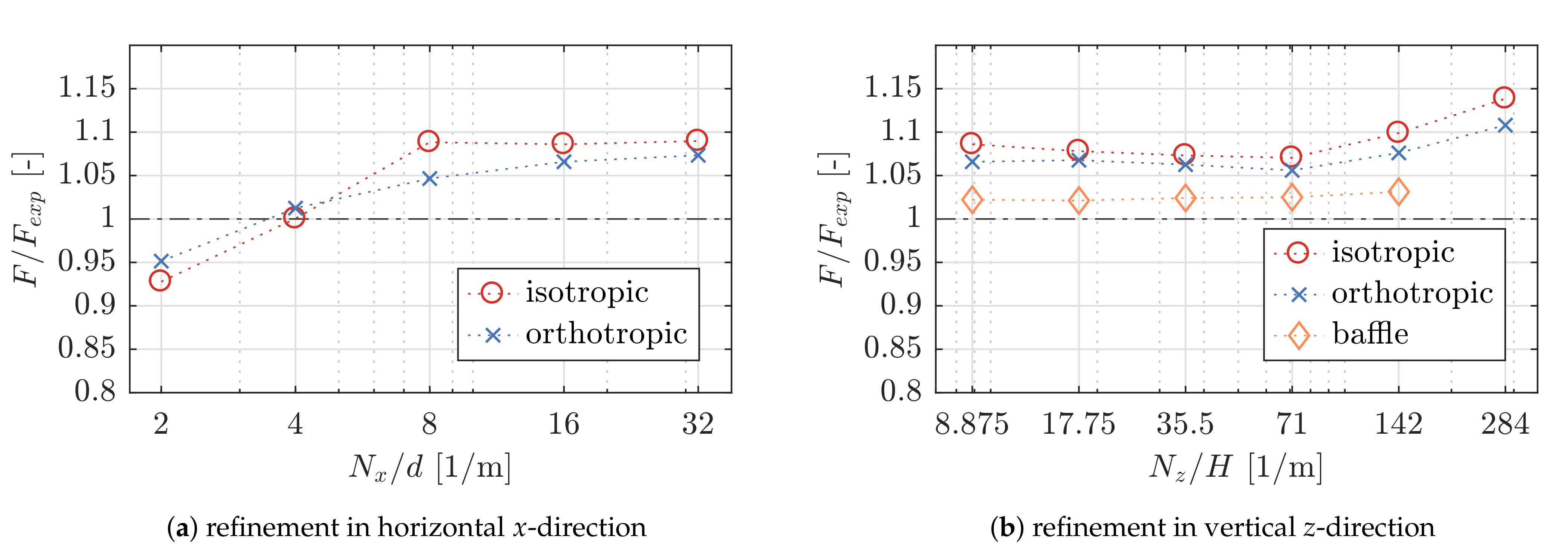Figure 5 shows the normalized force amplitude, $F/F_{exp}$, over the mesh refinement levels in terms of number of cells per sheet thickness in x-direction, $N_x/d$, and number of cells per wave height in z-direction, $N_z/H$. For the baffle implementation, the refinement level was only investigated in vertical z-direction as it has zero thickness. No result was obtained for 284 $N_z/H$, since the skewness of the cells would have been excessive. For all other models, highly skewed cells have been avoided.

Figure 5a indicates 8 cells per sheet thickness, $N_x/d$, results in a converged force amplitude, F, for an isotropic implementation. Further horizontal refinement has an insignificant effect on the result. For the orthotropic implementation, convergence can be observed towards 32 $N_x/d$. The difference between 16 and 32 $N_x/d$ is 3% relative to the smaller value. No clear convergence behaviour can be determined from Figure 5b for the number of cells per wave height in z-direction, $N_z/H$, for either of the implementations. It is not clear why the value of F in both porous-media implementations (isotropic and orthotropic) is seen to increase significantly for an increasing number of cells in the vertical direction, but this is suspected to be linked to the smeared nature of the air-water interface of the VOF interface capturing method. Although not presented in the figures here, the comparison of the velocity profiles along the water column for the gauges WG C1 and WG C2, 0.1 m before (x = 7.90 m) and 0.1 m after (x = 8.10 m) the sheet, confirm the results above. Based on the number of cells per sheet thickness, $N_x/d$, the profiles of the horizontal component, $u_x$, and the profiles of the vertical velocity component, $u_z$, require a minimum of 8 $N_x/d$ for the isotropic and 16 $N_x/d$ for the orthotropic implementation, to achieve a reasonable converged profile in front of the sheet at WG C1. The vertical mesh size, $N_z/H$, has barely any influence on the velocity profiles, $u_x$ and $u_z$, before and after the sheet for either the volumetric (isotropic and orthotropic) implementation and the baffle implementation. There are no significant differences after the sheet and only small deviations in front of it, where the largest deviations of $u_z$ are located along the free-surface. Overall, these differences are considered to be insignificant.

For the following models, a mesh resolution corresponding to 16 $N_x/d$ and 8.875 $N_z/H$ was used for all volumetric models (both isotropic and orthotropic) and 8.875 $N_z/H$ has been used for the models with the porous baffle. These values can serve as a guide for similar structures and wave conditions, but the dependence is likely to change for different conditions, in particular for significantly deviating wave conditions.

5.2. Horizontal Force on the Structures

In this section, the time series of the horizontal forces on both the sheet and cylinder are assessed as the main parameters of interest.

5.2.1. Force on the 2D Sheet

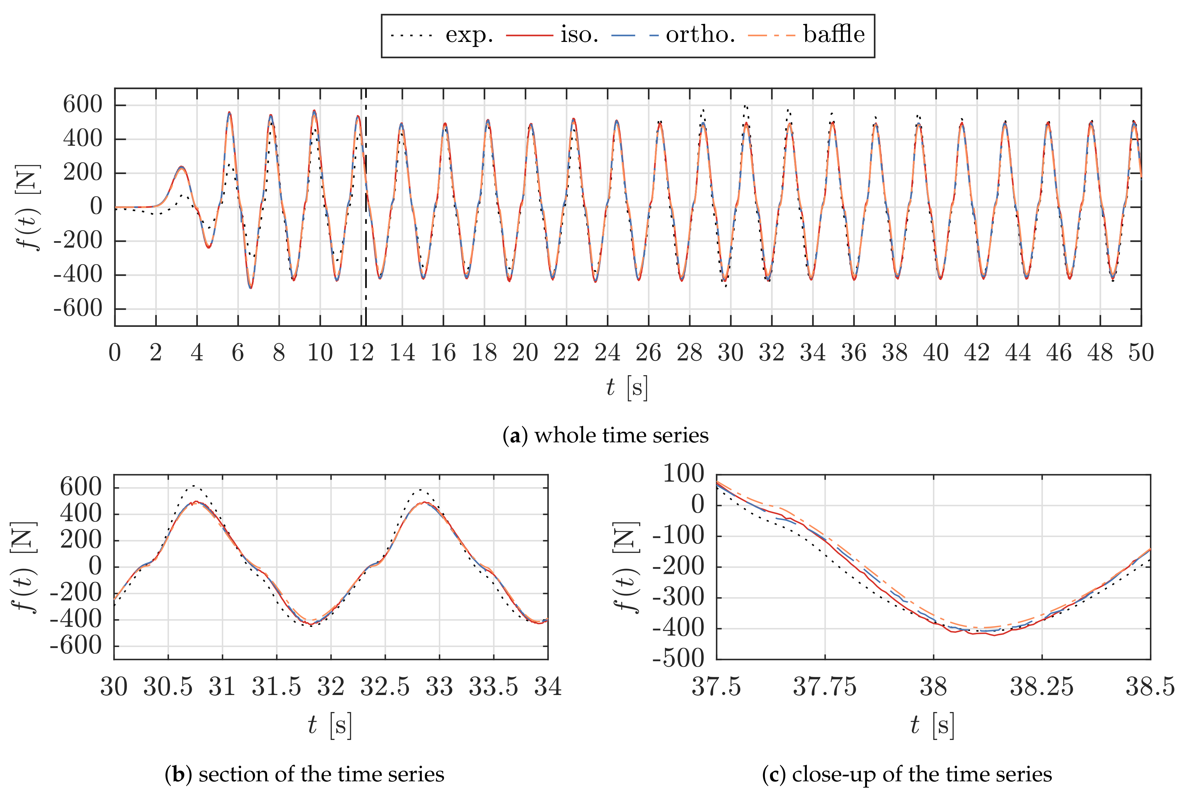
As before, the force on the 2D sheet has been scaled to match the width used in the experiments. A comparison between the time series of the horizontal force, $f\left(t\right)$, due to the different types of porosity implementation, is shown in Figure 6. The vertical line indicates the point in time when the wave has travelled across the tank and back to the center.

All types of porosity implementation are capable of reproducing the shape of the time series, which exhibits a non-sinusoidal shape due to the quadratic pressure-drop. The notable deviations between the CFD and experimental results for the initial transient section of the time series in Figure 6a are due to differences in the wave ramp-up between the numerical model and the physical wavemaker. The deviations concerning the wave ramp-up have been discussed in previous work, [33], where the free surface elevation has been validated for a range of regular wave conditions and porosities. The experimental results are slightly contaminated with wave reflections, shown for a section of the time series in Figure 6b. The numerical results exhibit a clean periodically steady-state after about t = 24 s. The numerical results agree well among each other, where only minor deviations can be observed at small local sections of the signal, which is outlined for an example in Figure 6c. The mean force amplitudes, F, of the CFD results are 391.19 N for the baffle implementation ($F/F_{exp}$ = 1.024), 407.84 N for the orthotropic implementation ($F/F_{exp}$ = 1.066) and 415.54 N for the isotropic implementation ($F/F_{exp}$ = 1.086).

5.2.2. Force on the Cylinder

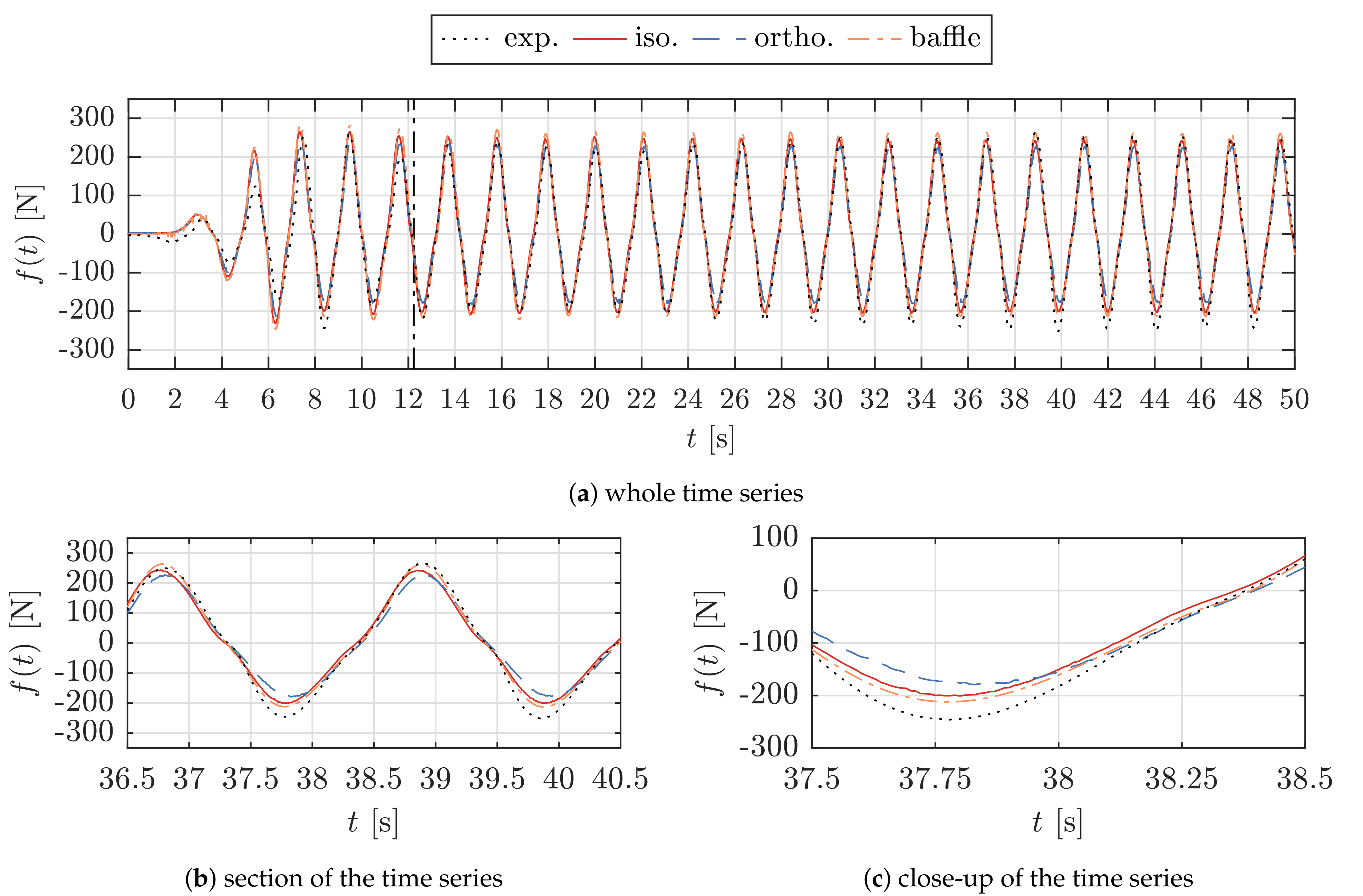
Next the results of the horizontal force on the cylinder are assessed and the time series, $f\left(t\right)$, are shown in Figure 7.

For the cylinder model, the initial transient period of the wave ramp-up also differs between the numerical and experimental results, and as before, the experimental results exhibit larger unsteadiness than the numerical results, due to wave reflections. The non-linearity of the force on the cylinder is replicated by all CFD models and all types of porosity implementations. The overall force response is reproduced with reasonably good agreement between the numerical and experimental results, as shown in Figure 7a. However, the deviations among the numerical results are larger for the cylinder than for the 2D sheet. The baffle implementation and the isotropic porous-media implementation agree well, but the orthotropic porous-media implementation deviates more notably. This can be observed for a section and close-up of the time series in the Figure 7b,c. The mean force amplitudes, F, of the CFD results are 218.63 N for the baffle implementation ($F/F_{exp}$ = 1.108 where $F_{exp}$ = 197.36 N), 188.81 N for the orthotropic implementation ($F/F_{exp}$ = 0.957) and 205.01 N for the isotropic implementation ($F/F_{exp}$ = 1.039).

5.3. Wave Gauges near the Structures

Next, the wave elevation, $\eta \left(t\right)$, at the WGs close to the structures is assessed. Here the whole time series for a physical runtime of 50 s and close-ups of sections of the time series are presented. Again, the vertical lines indicate the point in time when the wave has travelled across the tank and back to the WG.

5.3.1. Wave Gauges near the 2D Sheet

The analysis of the WG results for the 2D model with the sheet focuses on the comparison among the CFD results. The comparison against the experimental results is omitted since the latter are suspected to be unreliable due to a raised section of the floor in the physical tank which was required to submerge the load cells beneath the structures. For more information on this issue, we refer to previous discussions in [33,40].

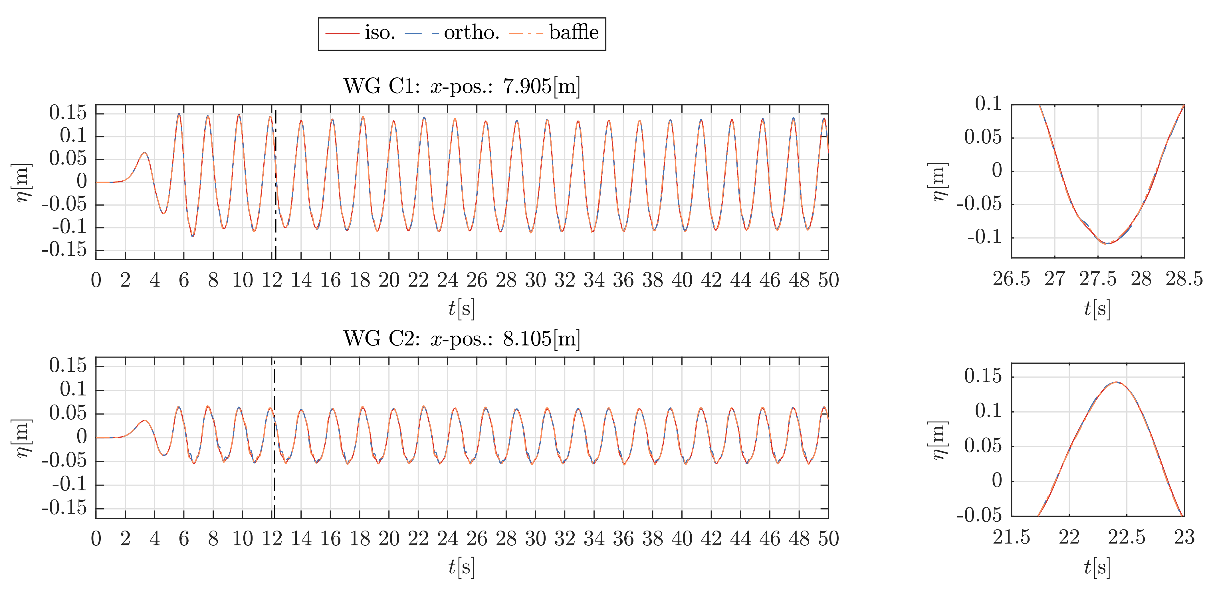
Figure 8 shows the water surface elevation, $\eta \left(t\right)$, for the WGs C1 and C2, which are placed 0.1 m before and 0.1 m after the sheet respectively, for all types of porosity representations.

The time series match very well among all CFD results and for all types of porosity implementation. In particular, the close-ups exhibit that the results are nearly identical, both before and after the sheet. At WG C1, 0.1 m before the sheet, the mean wave amplitudes, A, are 0.1189 m for the baffle implementation ($A/A_{input}$ = 1.340 where $A_{input}$ = 0.08875 m), 0.1200 m for the orthotropic implementation ($A/A_{input}$ = 1.352) and 0.1196 m for the isotropic implementation ($A/A_{input}$ = 1.348). At WG C2, 0.1 m after the sheet, A is 0.0595 m for the baffle implementation ($A/A_{input}$ = 0.6704), 0.0580 m for the orthotropic implementation ($A/A_{input}$=0.6535) and 0.0583 m for the isotropic implementation ($A/A_{input}$ = 0.6565).

5.3.2. Wave Gauges near the Cylinder

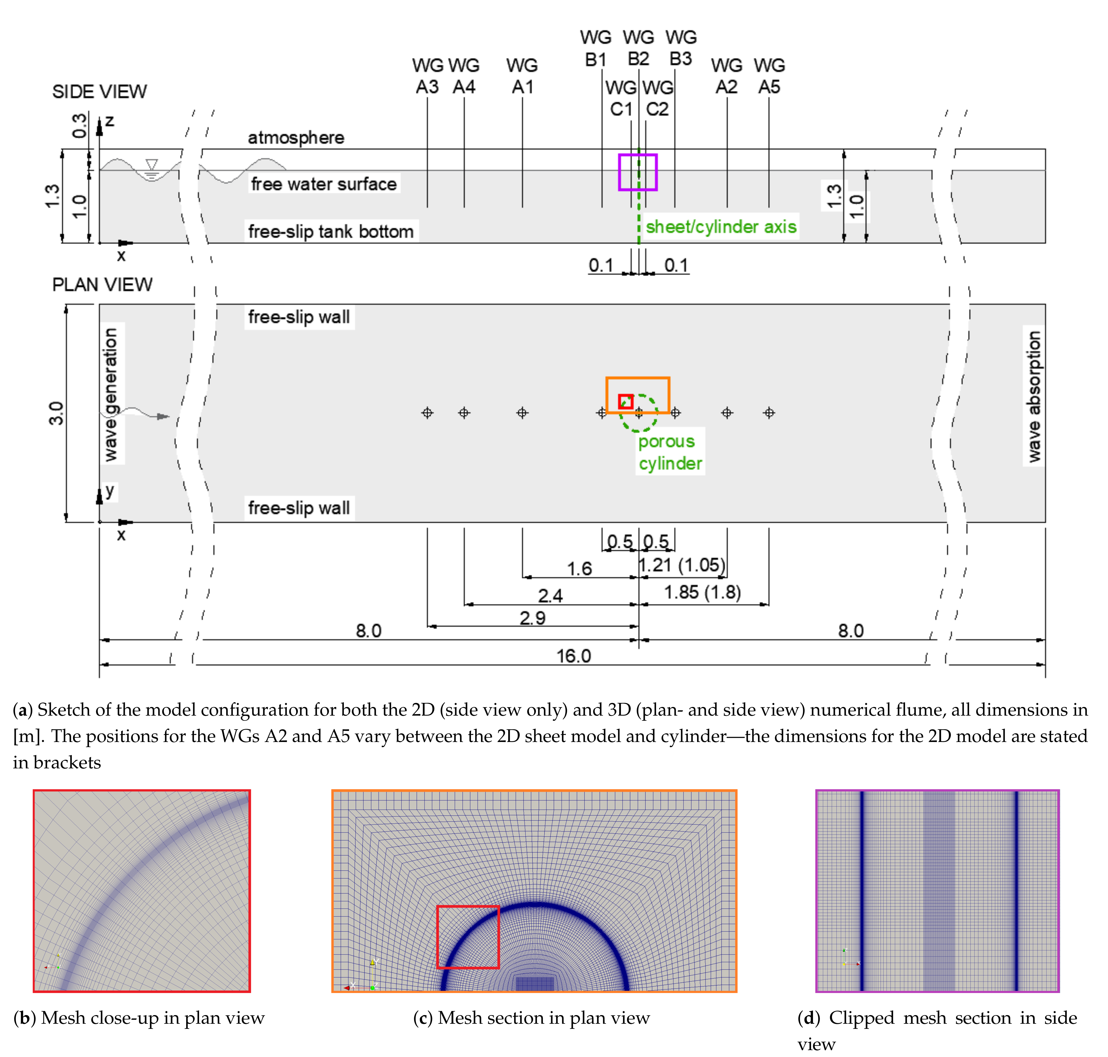
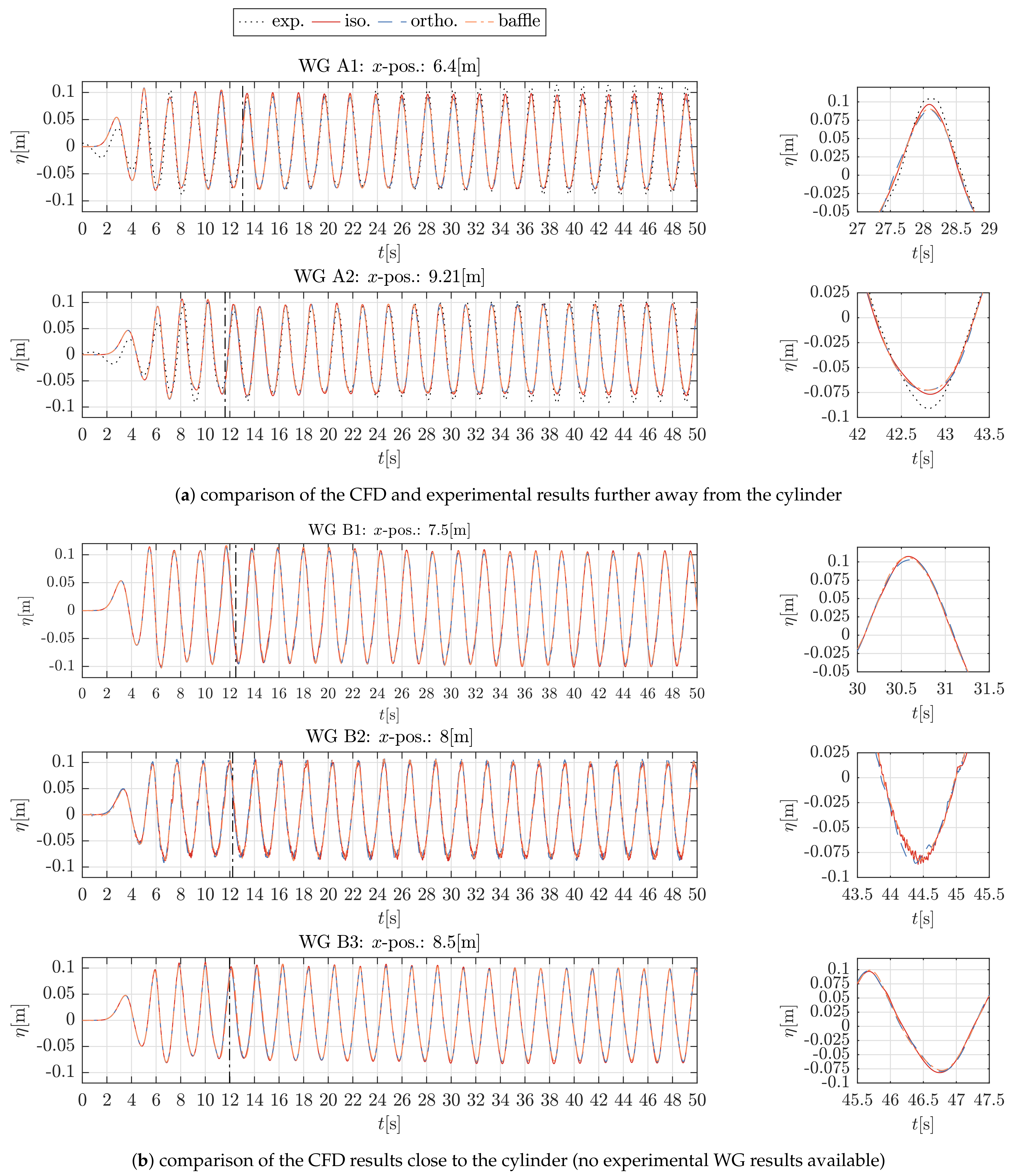
For the 3D model with the cylinder, the analysis covers the comparison among the CFD results and against the experimental data. Figure 9 presents the wave elevation, $\eta \left(t\right)$, for the WGs shown in Figure 3a. Figure 9a shows the WG signals from the numerical results due to all types of porosity implementation and the experimental results further away from the cylinder. Figure 9b shows the WG results closer to the cylinder where WG B1 is positioned 0.5 m before the cylinder axis, WG B3 0.5m behind the cylinder axis and WG B2 at the cylinder axis and at the center of the cylinder, respectively.

Similar to the time series of the force results, the figures exhibit differences at the initial transient section and wave reflections in the experimental results. Again, the overall agreement between CFD and experimental results is relatively good. The most noticeable differences can be observed between the CFD results for WG A1, positioned 1.6 m before the cylinder (Figure 9a). The isotropic implementation produces larger amplitudes after the wave has travelled across the tank and back to the centre. For the WG A2, 1.21 m after the cylinder, the results match very well. The time series for the WG B2 in the center of the cylinder exhibits small ripples for all types of porosity implementation. The ripples are suspected to be a result of instabilities in the VOF phase-fraction ($\alpha$)-field and to be related to the very fine mesh in the cylinder centre due to mesh generation procedures.

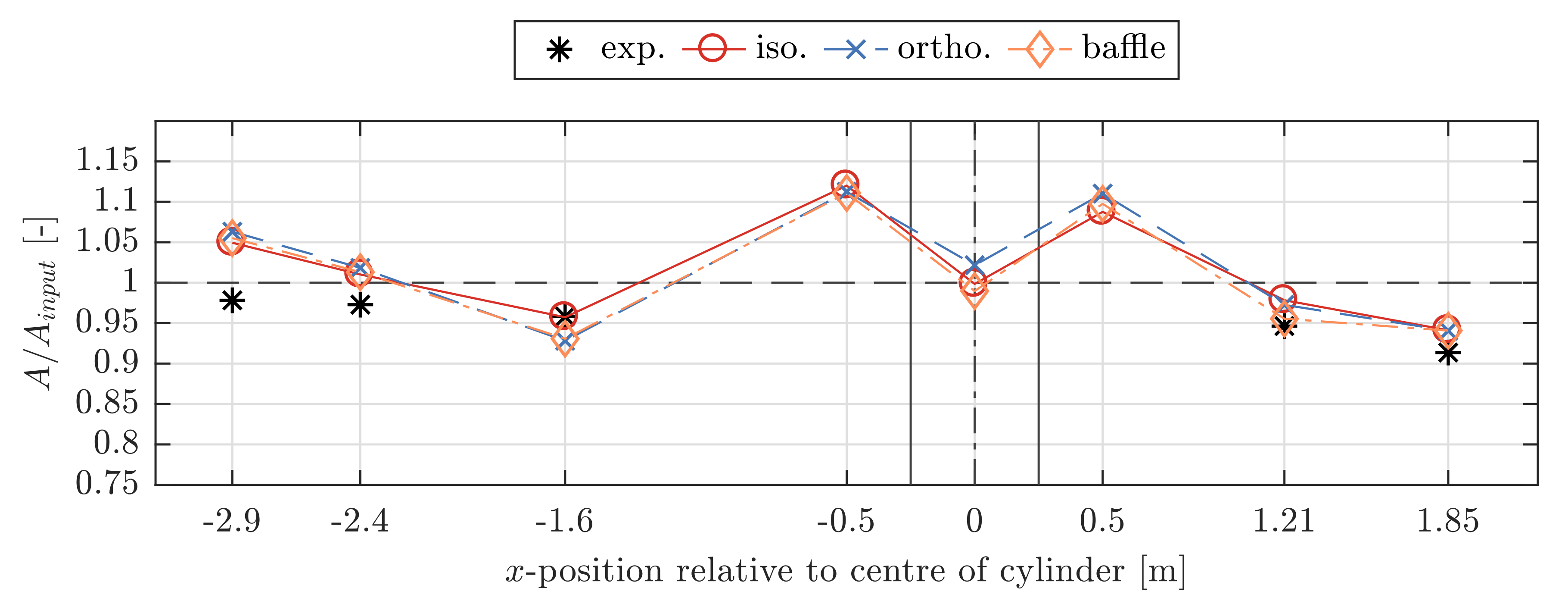
Next, the normalized mean wave amplitudes, $A/A_{input}$, where $A_{input}$ = 0.08875 m is the CFD wave amplitude input, are analysed for all WG positions and all types of porosity implementations. The comparison between the mean amplitude results is shown in Figure 10. For the WGs A1–A5, experimental results are included; for the WGs B1–B3, only CFD results are available.

The qualitative agreement between the experimental and all CFD results is relatively good at all WG positions. The deviations among the CFD results are small and do not exhibit clear patterns. The largest deviation of the mean amplitudes, A, among the CFD results is given at WG B2 in the centre of the tank at an x-position of 8.0 m. There, the largest value of A = 0.0907 m was obtained for the model with orthotropic porosity implementation. This results in a 3.23% larger value than the smallest value of A = 0.0878 m from the model with a porous baffle implementation. The smallest deviation has been obtained for the WG A5, 1.85 m after the cylinder centre at an x-position of 9.85 m, where all values result in a mean amplitude of A = 0.0835 m ($A/A_{input}$ = 0.9408).

5.4. Velocity Profiles near the Structures

The velocity profiles are assessed by means of a comparison between the CFD results from models with different types of porosity implementations. The positions of the velocity profiles correspond to the WG positions around both the sheet and cylinder; see Figure 3a. A limited number of selected profiles and points in time are presented for one wave trough and one wave crest each. These indicate the overall trend of results.

5.4.1. Velocity Profiles near the 2D Sheet

Figure 11 shows examples of the velocity profiles of the horizontal component, $u_x$, and the vertical component, $u_z$, with a distance of 0.1 m before (WG C1) and after (WG C2) the sheet. The dashed black horizontal lines indicate the mean water surface level with a water depth of h = 1.0 m. The continuous coloured horizontal lines represent the instantaneous water level at a specific time step. Both the horizontal and vertical velocity profiles, $u_x$ and $u_z$, cover the whole water column and a section of the air phase above the water level.

It can be observed that the largest differences are present for the horizontal velocities, $u_x$, along the air-water interface, with the largest values in the air just above the water surface. Some local high velocities are unphysical and a direct result of the large pressure and density gradients at the phase interface due to the segregated solution algorithm for the pressure-velocity coupling. The occurrence of spurious air velocities is well-known in the context of gravity wave propagation and has previously been reported by [59,60,61,62,63,64,65] related to the use of interFoam with its standard (MULES) VOF method.

Excluding the profile section in the air from the analysis, the agreement of the profiles in the water column match with insignificant differences for both the horizontal and vertical component, $u_x$ and $u_z$. The largest deviations have been obtained for the vertical velocity profile, $u_z$, 0.1 m after the sheet.

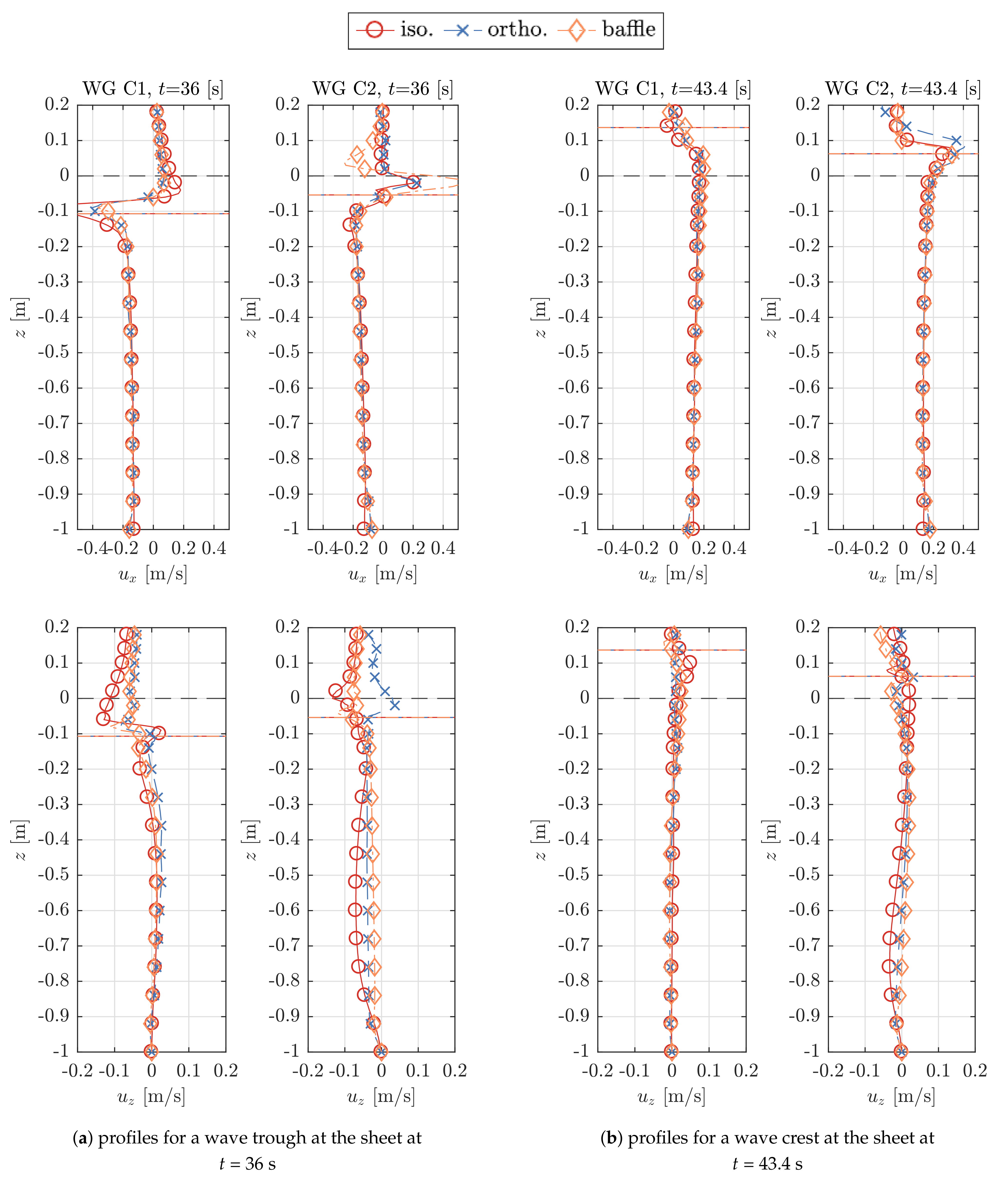
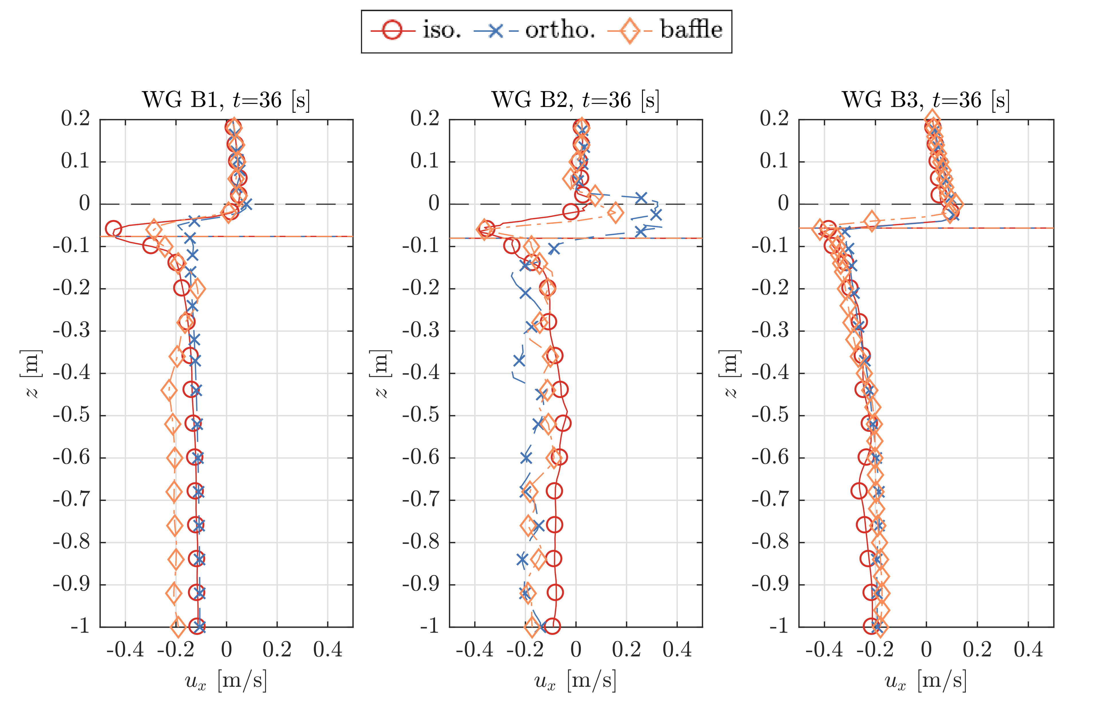
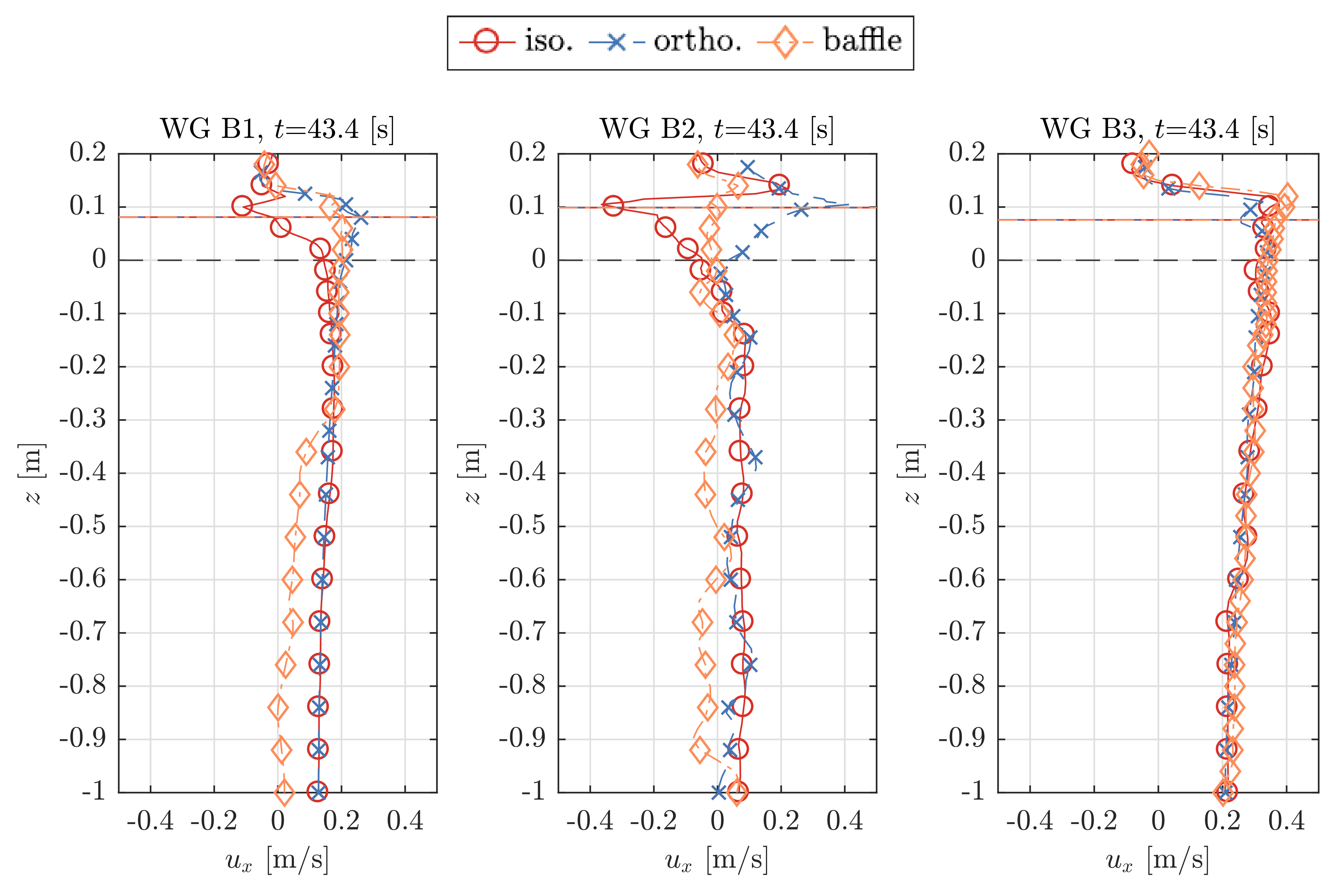
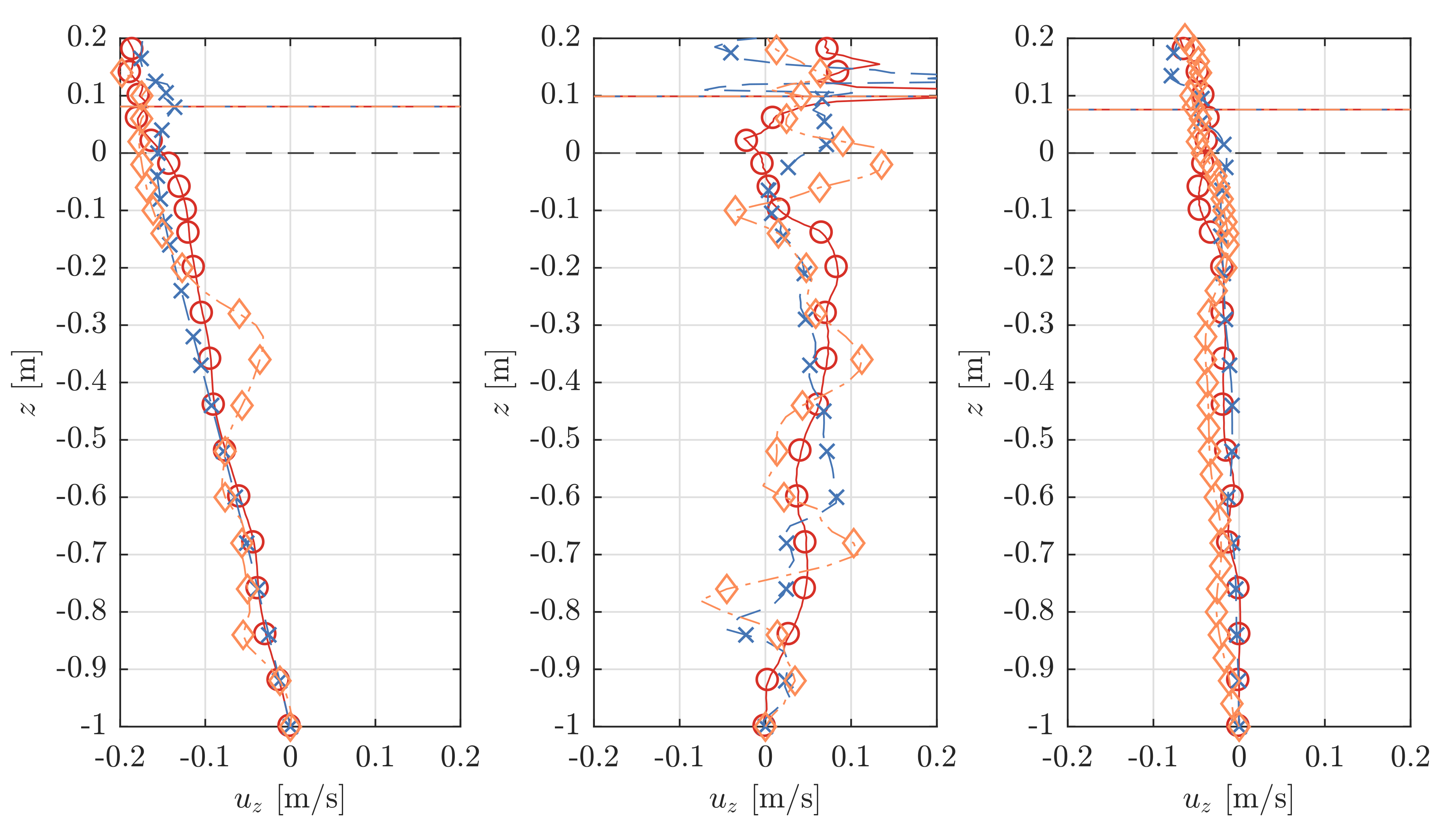
5.4.2. Velocity Profiles near the Cylinder

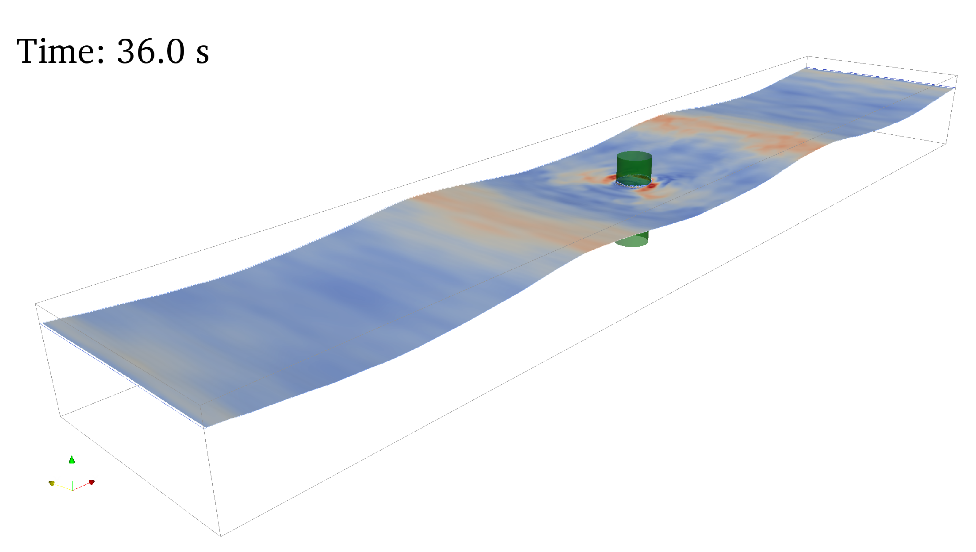
Figure 12 shows the velocity profiles, $u_x$ and $u_z$, for t = 36.0 s, where a wave trough passes the cylinder centre. Figure 13 shows the same for t = 43.4 s at a wave crest. Again, the dashed black and coloured horizontal lines indicate the initial flat and the instantaneous water level respectively.

Both Figure 12 and Figure 13 indicate similar patterns of locally large velocity values close to the air-water interface. The overall differences between the results due to the different porosity implementations are relatively small, both before (WG B1) and after (WG B3) the cylinder. At the cylinder center at WG B2, the profiles exhibit significant scatter for both the horizontal and vertical component, $u_x$ and $u_z$, so no clear trend can be identified from these results.

The differences between the results are the smallest for WG B3 after the cylinder and 0.5 m after the cylinder axis, respectively. At WG B1, 0.5 m in front of the cylinder axis, the profiles obtained from the porous-media models, both isotropic and orthotropic, match with insignificant deviations. The profiles due to the baffle-implementation deviate more notably from both porous-media implementations.

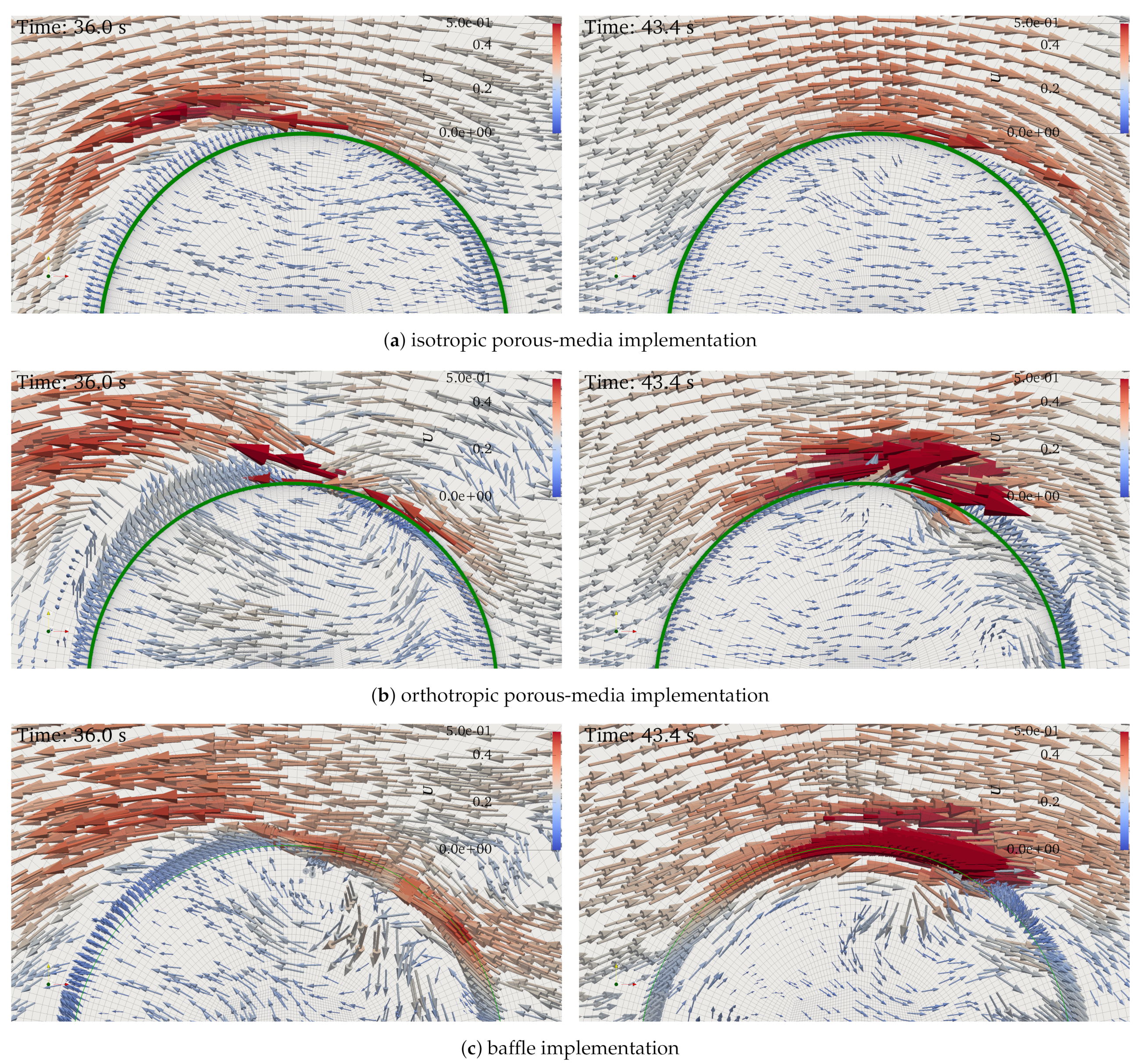
5.5. Flow Visualization near the Cylinder

To assess potential differences between the flow field due to different types of porosity implementations, the velocity vectors have been inspected qualitatively on a horizontal cross section across half of the cylinder. The cross-section is represented by a 50 mm thick horizontal slice of the domain that ranges from z = 0.75–0.80 m. The initial flat water level was at $z=h$ = 1.0 m. In Figure 14, the velocity vectors are shown for all types of investigated porosity implementations for two points in time. On the left, the flow field is presented for t = 36.0 s, which corresponds to a wave trough at the cylinder centre and on the right for t = 43.4 s, which corresponds to a wave crest.

Despite the very good agreement between all numerical results in terms of the force response and the flow field further away from the structures, differences are present for the flow field very close to the structure. From a qualitative point of view, the isotropic porosity implementation seems to produce flow patterns that are smoother compared to the orthotropic porous media and porous-baffle methods. In particular, the orthotropic implementation creates a more chaotic flow field and higher local velocities (for exactly the same mesh as the isotropic implementation), see Figure 14b. This could explain the reason for the requirement of smaller time steps in order to meet the target maximum $CFL$ number during the automatic time stepping process—which increases the computation time for the orthotropic implementation. The flow patterns agree better between the isotropic porous-media and the baffle implementation, see Figure 14a,c. This corresponds to a better match of the force results between the isotropic and baffle implementations, see Figure 7. The orthotropic implementation results in larger deviations for both the force results and the qualitative flow field, Figure 14b.

5.6. Tabular Summary of the Results

A summary of the main results is given in

Table 2. Summary of the normalized mean force amplitude results, $F/F_{exp}$, and the normalized mean wave amplitude results, $A/A_{input}$ at the WGs, including mesh cell number and execution times for all models.

Model	2D Sheet			3D Cylinder
Porosity Impl.	Isotropic	Orthotropic	Baffle	Isotropic	Orthotropic	Baffle
Number of Cells	68,890	68,890	68,060	9,840,065	9,840,065	7,192,448
Max. $CFL$	0.3	0.3	0.05	0.3	0.3	0.05
Used CPUs	1	1	1	28	28	28
Execution Time	6.6 h	7.8 h	1 d 9.9 h	8 d 14.1 h	13 d 2.7 h	72 d 17 h
$F/Fexp$	1.0860	1.0659	1.0242	1.0388	0.9567	1.1078
$A/A_{input}$ WG A1	0.6541	0.6556	0.6867	0.9573	0.9282	0.9307
$A/A_{input}$ WG A2	0.6395	0.6413	0.6596	0.9783	0.9406	0.9408
$A/A_{input}$ WG A3	1.3073	1.3117	1.3054	1.0494	1.0630	1.0552
$A/A_{input}$ WG A4	1.2073	1.2028	1.2066	1.0202	1.0184	1.0130
$A/A_{input}$ WG A5	0.6334	0.6370	0.6570	0.9412	0.9406	0.9408
$A/A_{input}$ WG B1	-	-	-	1.1201	1.1125	1.1109
$A/A_{input}$ WG B2	-	-	-	0.9985	1.0216	0.9897
$A/A_{input}$ WG B3	-	-	-	1.0877	1.1102	1.0975
$A/A_{input}$ WG C1	1.3476	1.3521	1.3397	-	-	-
$A/A_{input}$ WG C2	0.6569	0.6535	0.6704	-	-	-

. It shows the results of the mean force amplitudes, F, and the mean wave amplitudes, A, at the wave gauges for both the 2D and 3D model and includes the mesh cell number and approximate execution times for each model due to the different porosity implementations.

All models were simulated for 50 s of physical run time on 14-core dual Intel(R) Xeon(R) Gold 5120 CPU @ 2.20 GHz processors. The 2D models with the sheet were run on a single core. For 3D models with the cylinder, 28 CPUs were used.

6. Discussion

The overall results indicate that all types of investigated porosity implementations are capable of reproducing the horizontal force on the structures and the overall flow behaviour around the structures. The differences between the implementations are small for both the force and fluid flow results.

In particular, for the 2D model with the vertical sheet, all results are close to being identical for all types of porosity implementation. Only the vertical velocity profiles, $u_z$, exhibit small deviations for the WG C2, 0.1 m after the sheet, see Figure 11. The results of the model with the cylinder exhibit small deviations. In terms of horizontal force amplitude, F, the isotropic porous-media and porous-baffle implementation match reasonably well, and the orthotropic porous-media implementation leads to a slightly smaller value, see Figure 7a. No clear patterns can be determined for the mean flow behaviour in terms of wave elevation signals, $\eta \left(t\right)$ (Figure 9b), and mean wave amplitude, A (Figure 10). The velocity profiles close to the cylinder, $u_x$ and $u_z$, exhibit agreement between all different types of implementation 0.5 m after the cylinder at WG B3, see Figure 12 and Figure 13. Moreover, 0.5 m in front of the cylinder axis at WG B1 both porous-media implementations match relatively well, but the baffle implementation results in small deviations, in particular for the horizontal velocity component, $u_x$.

In contrast to similar work on fish cage structures, [1,2,36,37], the present work uses and compares three types of implementations in combination with a simpler pressure-drop model and momentum source formulation, respectively. The pressure-drop formulation does not require any calibration procedures or derivations from experimental results. Its validity has been demonstrated in combination with an isotropic porous-media implementation in previous work, [33], where also the general limitations of a macro-scale representation have been discussed. However, the present formulation has only been validated for thin structures with circular perforations, rather than net structures. Validation of the present method would need further validation for other types of porous barriers.

For the present case of thin perforated structures, we consider all types of implementations as suitable in principle. However, differences in numerical stability and execution times have been observed. While the solution process of all models with porous media-implementations maintained stability with a target maximum $CFL$-number of 0.3, the models with the baffle-implementation required very small time steps and a maximum $CFL$-number of 0.05 for a stable and unsupervised computation. Since the baffle implementation is usually reported to be more stable than the porous-media implementation in single-phase flow, e.g., by Shim et al. [2], we suspect that the instabilities are caused by the spurious air velocities at the interface, as already discussed in Section 5.4 in terms of their effect on the velocity profiles. Excessive velocity spikes at the sheet would directly lead to a spike in the pressure-drop source since it is a function of velocity, Equation (1), which can cause the solver to diverge and crash. We assume that the spurious velocities impact the baffle implementation significantly, but do not affect the porous-media implementations as much, because the smeared pressure-drop application over a volumetric porous zone possibly helps to avoid excessive pressure spikes. The baffle implementation is considered as disadvantageous for this specific numerical framework, using an algebraic VOF method and a segregated pressure-velocity coupling algorithm, and the present application of two-phase wave-structure interaction. The small time steps increase the computation times significantly. However, this problem could be resolved with a different interface capturing method or a different solver algorithm. Furthermore, the execution time of the isotropic implementation is shorter than the orthotropic porous-media implementation, see Section 4.2. Despite both models being set up with the identical mesh and same scheme and solver settings, the orthotropic implementation requires smaller time steps to meet the maximum target $CFL$ number. It is suspected that this is caused by more chaotic flow patterns with higher local velocity values that result from the orthotropic implementation, see Figure 14b.

While all types of implementations are capable of reproducing the forces and overall flow fields for the specific present conditions, the applicability of each type would need to be assessed for more general cases. It would, in particular, be interesting to assess the threshold of the thickness of the porous barrier at which the current pressure-drop model and the implementations are still valid.

7. Conclusions

This work presents an assessment of possible differences between different types of macro-scale porosity representation of thin perforated structures for CFD modelling of wave-structure interaction. The types of macro-scale representation are implementations as porous surface with a pressure-jump condition and as volumetric porous-media, one with the assumption of isotropic properties and one with orthotropic characteristics.

2D models of regular wave interaction with a vertical bottom-fixed porous sheet and 3D models with a bottom-fixed porous cylinder are simulated. The numerical results are compared against experimental results, but the focus lies on the direct comparison between the CFD results by means of the global force on the structure and the mean flow behaviour close to the structure. The latter is evaluated in terms of the free-surface elevation at wave gauges, velocity profiles along the water column and qualitative fluid flow visualizations.

The present assessment indicates that the differences between all types of investigated porosity implementations are insignificant when global forces and the overall flow behaviour are of interest. All models are capable of accurately reproducing the horizontal force on the structures and the overall fluid flow behaviour.

It was found that the implementation as porous baffle with a pressure-jump condition is numerically the most sensitive within the present numerical framework of a combination of the volume-of-fluid interface capturing method and a segregated pressure-velocity coupling algorithm. Adversely, very small time steps are required to avoid the generation of spurious air velocities above the water surface and their effect of causing pressure-drop spikes and solver divergence.

For the present specific conditions, we consider the isotropic porous-media implementation as the best option due to the following reasons. It is numerically stable and achieved the fastest execution times when it is used with automatic time-stepping. Its implementation is simple and does not require any considerations on directionality in comparison to the orthotropic porous-media implementation. It is capable of reproducing the mean force and fluid flow behaviour and is equally accurate as both the orthotropic porous-media and porous-baffle implementation.

This work can serve as a useful guide for CFD modelling of similar marine engineering problems of current and wave interaction with thin perforated structures.

References

1. Chen, H.; Christensen, E.D. Investigations on the porous resistance coefficients for fishing net structures. J. Fluids Struct. 2016, 65, 76–107. [Google Scholar] [CrossRef] [Green Version]
2. Shim, K.; Klebert, P.; Fredheim, A. Numerical investigation of the flow through and around a net cage. In Proceedings of the International Conference on Offshore Mechanics and Arctic Engineering, Honolulu, HI, USA, 31 May–5 June 2009; Volume 43444, pp. 581–587. [Google Scholar]
3. Lee, K.H.; Bae, J.H.; Kim, S.G.; Kim, D.S. Three-dimensional simulation of wave reflection and pressure acting on circular perforated caisson breakwater by OLAFOAM. J. Korean Soc. Coast. Ocean Eng. 2017, 29, 286–304. [Google Scholar] [CrossRef] [Green Version]
4. Valizadeh, A.; Rafiee, A.; Francis, V.; Rudman, M.; Ramakrishnan, B. An analysis of perforated plate breakwaters. In Proceedings of the Twenty-Eighth (2018) International Ocean and Polar Engineering Conference, Sapporo, Japan, 10–15 June 2018; pp. 1174–1180. [Google Scholar]
5. Tait, M.J. Modelling and preliminary design of a structure-TLD system. Eng. Struct. 2008, 30, 2644–2655. [Google Scholar] [CrossRef]
6. Tait, M.J.; El Damatty, A.A.; Isyumov, N.; Siddique, M.R. Numerical flow models to simulate tuned liquid dampers (TLD) with slat screens. J. Fluids Struct. 2005, 20, 1007–1023. [Google Scholar] [CrossRef]
7. Hamelin, J.A.; Love, J.S.; Tait, M.J.; Wilson, J.C. Tuned liquid dampers with a Keulegan-Carpenter number-dependent screen drag coefficient. J. Fluids Struct. 2013, 43, 271–286. [Google Scholar] [CrossRef]
8. Baker, M.; Young, P.; Tabor, G.R. Image based meshing of packed beds of cylinders at low aspect ratios using 3d MRI coupled with computational fluid dynamics. Comput. Chem. Eng. 2011, 35, 1969–1977. [Google Scholar] [CrossRef]
9. Baker, M.J.; Tabor, G.R. Computational analysis of transitional airflow through packed columns of spheres using the finite volume technique. Comput. Chem. Eng. 2010, 34, 878–885. [Google Scholar] [CrossRef] [Green Version]
10. Chen, B.; Wang, L.; Ning, D.; Johanning, L. CFD analysis on wave load mitigation effect of a perforated wall on offshore structure. In Proceedings of the Twenty-Ninth (2019) International Ocean and Polar Engineering Conference, Honolulu, HI, USA, 16–21 June 2019; pp. 3653–3658. [Google Scholar]
11. Poguluri, S.K.; Cho, I.H. Analytical and numerical study of wave interaction with a vertical slotted barrier. Ships Offshore Struct. 2020, 1–13. [Google Scholar] [CrossRef]
12. Fugazza, M.; Natale, L. Hydraulic design of perforated breakwaters. J. Waterw. Port Coast. Ocean Eng. 1992, 118, 1–14. [Google Scholar] [CrossRef]
13. Bennett, G.S.; McIver, P.; Smallman, J.V. A mathematical model of a slotted wavescreen breakwater. Coast. Eng. 1992, 18, 231–249. [Google Scholar] [CrossRef]
14. Hagiwara, K. Analysis of upright structure for wave dissipation using integral equation. In Proceedings of the 19th International Conference on Coastal Engineering, Houston, TX, USA, 3–7 September 1984; pp. 2810–2826. [Google Scholar]
15. Li, H.H.; Cheng, Y.Y. Effect of porous-jump model parameters on membrane flux prediction. In Advanced Materials Research; Trans. Tech. Publ.: Stafa-Zurich, Switzerland, 2013; Volume 734, pp. 2210–2213. [Google Scholar]
16. Arghode, V.K.; Joshi, Y. Modeling strategies for air flow through perforated tiles in a data center. IEEE Trans. Components Packag. Manuf. Technol. 2013, 3, 800–810. [Google Scholar] [CrossRef]
17. Chacko, S.; Shome, B.; Kumar, V.; Agarwal, A.; Katkar, D. Numerical simulation for improving radiator efficiency by air flow optimization. In Proceedings of the ANSA & ETA International Congress, Halkidiki, Greece, 2–3 June 2005. [Google Scholar]
18. Van der Spuy, S.J.; von Backström, T.W. An evaluation of simplified CFD models applied to perimeter fans in air-cooled steam condensers. Proc. Inst. Mech. Eng. Part A J. Power Energy 2015, 229, 948–967. [Google Scholar] [CrossRef]
19. Sumara, Z.; Šochman, M. CFD study on the effects of boundary conditions on air flow through an air-cooled condenser. EPJ Web Conf. 2018, 180, 1–5. [Google Scholar] [CrossRef]
20. Kizilaslan, M.A.; Demirel, E.; Aral, M.M. Effect of porous baffles on the energy performance of contact tanks in water treatment. Water 2018, 10, 1084. [Google Scholar] [CrossRef] [Green Version]
21. Wang, L.; Zhang, L.; Lian, G. A CFD simulation of 3D air flow and temperature variation in refrigeration cabinet. Procedia Eng. 2015, 102, 1599–1611. [Google Scholar] [CrossRef] [Green Version]
22. Shen, X.; Wang, T.; Zhong, W. Numerical simulation and wake modeling of wind turbine rotor as an actuator disk. Int. J. Mod. Phys. Conf. Ser. 2012, 19, 320–330. [Google Scholar] [CrossRef]
23. Hunter, W. Actuator Disk Methods for Tidal Turbine Arrays. Ph.D. Thesis, University of Oxford, Oxford, UK, 2015. [Google Scholar]
24. Bakica, A.; Gatin, I.; Vukčević, V.; Jasak, H.; Vladimir, N. Accurate assessment of ship-propulsion characteristics using CFD. Ocean Eng. 2019, 175, 149–162. [Google Scholar] [CrossRef]
25. Barakos, G.N.; Fitzgibbon, T.; Kusyumov, A.N.; Kusyumov, S.A.; Mikhailov, S.A. CFD simulation of helicopter rotor flow based on unsteady actuator disk model. Chin. J. Aeronaut. 2020, 33, 2313–2328. [Google Scholar] [CrossRef]
26. Filippone, A.; Mikkelsen, R. Advances in CFD & actuator disk models for helicopter aerodynamics. In Proceedings of the 35th European Rotorcraft Forum 2009, ERF 2009, Hamburg, Germany, 22–25 September 2009; Volume 2, pp. 661–669. [Google Scholar]
27. Higuera, P.; Lara, J.; Losada, I. Three-dimensional interaction of waves and porous coastal structures using OpenFOAM. Part I: Formulation and validation. Coast. Eng. 2014, 83, 243–258. [Google Scholar] [CrossRef]
28. Lara, J.L.; del Jesus, M.; Losada, I.J. Three-dimensional interaction of waves and porous coastal structures Part II: Experimental validation. Coast. Eng. 2012, 64, 26–46. [Google Scholar] [CrossRef]
29. Del Jesus, M.; Lara, J.L.; Losada, I.J. Three-dimensional interaction of waves and porous coastal structures Part I: Numerical model formulation. Coast. Eng. 2012, 64, 57–72. [Google Scholar] [CrossRef]
30. Brito, M.; Fernandes, J.; Leal, J.B. Porous media approach for RANS simulation of compound open-channel flows with submerged vegetated floodplains. Environ. Fluid Mech. 2016, 6, 1247–1266. [Google Scholar] [CrossRef] [Green Version]
31. Hadadpour, S.; Paul, M.; Oumeraci, H. Numerical investigation of wave attenuation by rigid vegetation based on a porous media approach. J. Coast. Res. 2019, 92, 92–100. [Google Scholar] [CrossRef]
32. Feichtner, A.; Mackay, E.; Tabor, G.; Thies, P.R.; Johanning, L. Modelling wave interaction with thin porous structures using OpenFOAM. In Proceedings of the 13th European Wave and Tidal Energy Conference (EWTEC 2019), Napoli, Italy, 1–6 September 2019. [Google Scholar]
33. Feichtner, A.; Mackay, E.; Tabor, G.; Thies, P.R.; Johanning, L.; Ning, D. Using a porous-media approach for CFD modelling of wave interaction with thin perforated structures. J. Ocean. Eng. Mar. Energy 2020, 6, 1–23. [Google Scholar] [CrossRef]
34. Qiao, D.; Feng, C.; Yan, J.; Liang, H.; Ning, D.; Li, B. Numerical simulation and experimental analysis of wave interaction with a porous plate. Ocean Eng. 2020, 218, 108106. [Google Scholar] [CrossRef]
35. Kyte, A. Practical use of computational fluid dynamics (CFD) in improving the efficiency of domestic ventilation waste heat recovery systems. Int. J. Energy Environ. Eng. 2014, 5, 1–7. [Google Scholar] [CrossRef] [Green Version]
36. Zhao, Y.P.; Bi, C.W.; Dong, G.H.; Gui, F.K.; Cui, Y.; Guan, C.T.; Xu, T.J. Numerical simulation of the flow around fishing plane nets using the porous media model. Ocean Eng. 2013, 62, 25–37. [Google Scholar] [CrossRef]
37. Zhao, Y.P.; Bi, C.W.; Liu, Y.X.; Dong, G.H.; Gui, F.K. Numerical simulation of interaction between waves and net panel using porous media model. Eng. Appl. Comput. Fluid Mech. 2014, 8, 116–126. [Google Scholar] [CrossRef] [Green Version]
38. Hafsteinsson, H.E. Porous Media in OpenFOAM; Technical Report; Chalmers: Gothenburg, Sweden, 2009. [Google Scholar]
39. Jensen, B.; Jacobsen, N.G.; Christensen, E.D. Investigations on the porous media equations and resistance coefficients for coastal structures. Coast. Eng. 2014, 84, 56–72. [Google Scholar] [CrossRef]
40. Mackay, E.; Johanning, L.; Qiao, D.; Ning, D. Numerical and experimental modelling of wave loads on thin porous sheets. In Proceedings of the ASME 2019 38th International Conference on Ocean, Offshore and Arctic Engineering, Glasgow, Scotland, 9–14 June 2019. [Google Scholar]
41. Mackay, E.; Shi, W.; Qiao, D.; Gabl, R.; Davey, T.; Ning, D.; Johanning, L. Numerical and experimental modelling of wave interaction with fixed and floating porous cylinders. Preprint 2020, 10. [Google Scholar]
42. Sollitt, C.K.; Cross, R.H. Wave transmission through permeable breakwaters. Coast. Eng. 1972, 1, 1827–1846. [Google Scholar] [CrossRef] [Green Version]
43. Molin, B. Hydrodynamic modeling of perforated structures. Appl. Ocean Res. 2011, 33, 1–11. [Google Scholar] [CrossRef]
44. Weller, H.G.; Tabor, G.; Jasak, H.; Fureby, C. A Tensorial Approach to Computational Continuum Mechanics using Object Orientated Techniques. Comput. Phys. 1998, 12, 620–631. [Google Scholar] [CrossRef]
45. Deshpande, S.S.; Anumolu, L.; Trujillo, M.F. Evaluating the performance of the two-phase flow solver interFoam. Comput. Sci. Discov. 2012, 5, 014016. [Google Scholar] [CrossRef]
46. The OpenFOAM Foundation. OpenFOAM v5 User Guide. Available online: https://cfd.direct/openfoam/user-guide (accessed on 28 December 2020).
47. Berberovic, E.; Hinsberg, N.P.V.; Jakirlic, S.; Roisman, I.V.; Tropea, C. Drop impact onto a liquid layer of finite thickness: Dynamics of the cavity evolution. Phys. Rev. E 2009, 79, 1–15. [Google Scholar] [CrossRef]
48. Higuera, P. OlaFlow: CFD for Waves [Software]. 2017. Available online: http://doi.org/10.5281/zenodo.1297013 (accessed on 28 December 2020).
49. Jacobsen, N.G.; Fuhrman, D.R.; Fredsoe, J. A wave generation toolbox for the open-source CFD library: OpenFoam. Int. J. Numer. Methods Fluids 2012, 70, 1073–1088. [Google Scholar] [CrossRef]
50. Gray, W.G. A derivation of the equations for multi-phase transport. Chem. Eng. Sci. 1975, 30, 229–233. [Google Scholar] [CrossRef]
51. Slattery, J.C. Flow of viscoelastic fluids through porous media. AIChE J. 1967, 13, 1066–1071. [Google Scholar] [CrossRef]
52. Withaker, S. The Forchheimer Equation: A Theoretical Development. Transp. Porous Media 1996, 25, 27–61. [Google Scholar] [CrossRef]
53. Moukalled, F.; Mangani, L.; Darwish, M. The Finite Volume Method in Computational Fluid Dynamics—An Advanced Introduction with OpenFOAM and Matlab; Springer: Heidelberg, Garmany, 2016; Volume 113, pp. 535–557. [Google Scholar] [CrossRef] [Green Version]
54. Chakrabarti, S.K. Hydrodynamics of Offshore Structures; WIT Press: Southampton, UK, 1987. [Google Scholar]
55. Sumer, B.M.; Christiansen, N.; Fredsøe, J. The horseshoe vortex and vortex shedding around a vertical wall-mounted cylinder exposed to waves. J. Fluid Mech. 1997, 332, 41–70. [Google Scholar] [CrossRef]
56. Fredsoe, J.; Sumer, B.M. Hydrodynamics around Cylindrical Structures, revised ed.; World Scientific: Singapore, 2006; Volume 26. [Google Scholar]
57. Higuera, P. Enhancing active wave absorption in RANS models. Appl. Ocean Res. 2019, 94, 102000. [Google Scholar] [CrossRef]
58. Mansard, E.; Funke, E. The measurement of incident and reflected spectra using a least squares method. In Proceedings of the 17th International Conference on Coastal Engineering, Sydney, Australia, 23–28 March 1980; pp. 154–172. [Google Scholar]
59. Vukčević, V. Numerical Modelling of Coupled Potential and Viscous Flow for Marine Applications. Ph.D. Thesis, University of Zagreb, Zagreb, Croatia, 2016. [Google Scholar] [CrossRef]
60. Vukčević, V.; Jasak, H.; Gatin, I. Implementation of the Ghost Fluid Method for free surface flows in polyhedral Finite Volume framework. Comput. Fluids 2017, 153, 1–19. [Google Scholar] [CrossRef]
61. Amini Afshar, M. Numerical Wave Generation In OpenFOAM®. Master’s Thesis, Chalmers University of Technology, Gothenburg, Sweden, 2010. [Google Scholar]
62. Roenby, J. A new volume-of-fluid method in OpenFOAM. In Proceedings of the MARINE 2017 Computational Methods in Marine Engineering VII Publication, Nantes, France, 15–17 May 2017; p. 13. [Google Scholar]
63. Larsen, B.E.; Fuhrman, D.R.; Roenby, J. Performance of interFoam on the simulation of progressive waves. Coast. Eng. J. 2019, 61, 380–400. [Google Scholar] [CrossRef] [Green Version]
64. Tomaselli, P.D. A Methodology for Air Entrainment in Breaking Waves and Their Interaction with a Mono-Pile. Ph.D. Thesis, Technical University of Denmark, Lyngby, Denmark, 2016. [Google Scholar]
65. Wroniszewski, P.A.; Verschaeve, J.C.; Pedersen, G.K. Benchmarking of Navier-Stokes codes for free surface simulations by means of a solitary wave. Coast. Eng. 2014, 91, 1–17. [Google Scholar] [CrossRef]
Figure 1. Options for porosity representation in computational fluid dynamics (CFD) modeling for thin porous structures.
Jmse 09 00150 g001
Figure 2. Schematics of the investigated porosity implementations, showing mesh cells and arrows that represent the velocity vectors close to a porous sheet; bold lines along the cell faces indicate the components of the velocity that are subject to a pressure-drop; shades represent porous-media zones. (a) isotropic (same resistance in x-, y- and z-direction) (b) orthotropic (resistance in x-direction) (c) baffle (resistance in normal direction to a surface).
Jmse 09 00150 g002
Figure 3. CFD model setup: (a) sketch of the model configuration for both the 2D and 3D numerical flume, (bd) sections of the mesh of the 3D model with the cylinder represented by porous media where (b,c) show sections in plan view and (d) the side view of a clip across the vertical xz symmetry plane. The colours of the rectangles in (a) correspond to the colours of the frames of (bd). (a) Sketch of the model configuration for both the 2D (side view only) and 3D (plan- and side view) numerical flume, all dimensions in [m]. The positions for the WGs A2 and A5 vary between the 2D sheet model and cylinder—the dimensions for the 2D model are stated in brackets (b) Mesh close-up in plan view (c) Mesh section in plan view (d) Clipped mesh section in side view.
Jmse 09 00150 g003
Figure 4. Snapshot of the 3D model where the porous cylinder is represented by orthotropic porous media. An animation of the wave-structure interaction is available as supplementary material.
Jmse 09 00150 g004
Figure 5. Mesh independence study for the normalized horizontal force on the 2D sheet, F/Fexp, separately for the number of (a) cells per sheet thickness (where d = 10 mm) in horizontal x-direction (Nx/d) and (b) cells per wave height (where H = 177.5 mm) in vertical z-direction (Nz/H), including the force results from models with all investigated porosity implementations. (a) refinement in horizontal x-direction (b) refinement in vertical z-direction.
Jmse 09 00150 g005
Figure 6. Comparison of the horizontal force on the porous 2D sheet, f(t), for the investigated types of porosity implementation. (a) whole time series (b) section of the time series (c) close-up of the time series.
Jmse 09 00150 g006
Figure 7. Comparison of the horizontal force on the cylinder, f(t), for the investigated types of porosity implementation. (a) whole time series (b) section of the time series (c) close-up of the time series.
Jmse 09 00150 g007
Figure 8. CFD results of the wave elevation, η ( t ) , at selected WGs close to the porous sheet for all types of porosity implementation, including the whole time series and selected close-ups.
Jmse 09 00150 g008
Figure 9. Experimental and CFD results of the wave elevation, η ( t ) , at selected WGs close to the porous cylinder for all types of porosity implementation, including the whole time series and selected close-ups. (a) comparison of the CFD and experimental results further away from the cylinder (b) comparison of the CFD results close to the cylinder (no experimental WG results available).
Jmse 09 00150 g009
Figure 10. CFD and experimental results of the normalized mean wave amplitudes, A / A i n p u t , for all WGs before and after the cylinder. The position of the center of the cylinder is indicated with a dashed vertical line and the cylinder front and back are indicated with solid vertical lines.
Jmse 09 00150 g010
Figure 11. Velocity profiles in horizontal, ux, and vertical, uz, direction 0.1 m before (WG C1) and 0.1 m after (WG C2) the sheet for a wave trough and crest at the sheet. (a) profiles for a wave trough at the sheet at t = 36 s (b) profiles for a wave crest at the sheet at t = 43.4 s.
Jmse 09 00150 g011
Figure 12. Velocity profiles in horizontal, u x , and vertical, u z , direction at the cylinder centre (WG B2), 0.5 m before (WG B1) and 0.5 m after (WG B3) the axis for a wave trough at the cylinder centre.
Jmse 09 00150 g012aJmse 09 00150 g012b
Figure 13. Velocity profiles in horizontal, u x , and vertical, u z , direction at the cylinder centre (WG B2), 0.5 m before (WG B1) and 0.5 m after (WG B3) the axis for a wave crest at the cylinder centre.
Jmse 09 00150 g013aJmse 09 00150 g013b
Figure 14. Velocity vectors for two points in time, t = 36.0 s at a wave trough (on the left) and t = 43.4 s at a wave crest (on the right) at the cylinder center. The waves propagate from the left to the right. The velocity magnitude and color of the vectors respectively ranges between 0.0–0.5 m/s. (a) isotropic porous-media implementation (b) orthotropic porous-media implementation (c) baffle implementation.
Jmse 09 00150 g014