Author Contributions
Conceptualization, P.T., C.C.S., N.T. and S.F.; Data curation, P.T., C.C.S. and N.T.; Formal analysis, P.T., C.C.S. and N.T.; Funding acquisition, C.G.; Investigation, P.T.; Methodology, P.T., C.C.S. and N.T.; Project administration, C.G.; Resources, C.G.; Software, P.T. and C.C.S.; Supervision, C.C.S., N.T. and S.F.; Validation, C.C.S., N.T. and S.F.; Visualization, P.T., C.C.S. and N.T.; Writing—original draft, P.T. and C.C.S.; Writing—review & editing, C.C.S., N.T., C.G. and S.F. All authors have read and agreed to the published version of the manuscript.
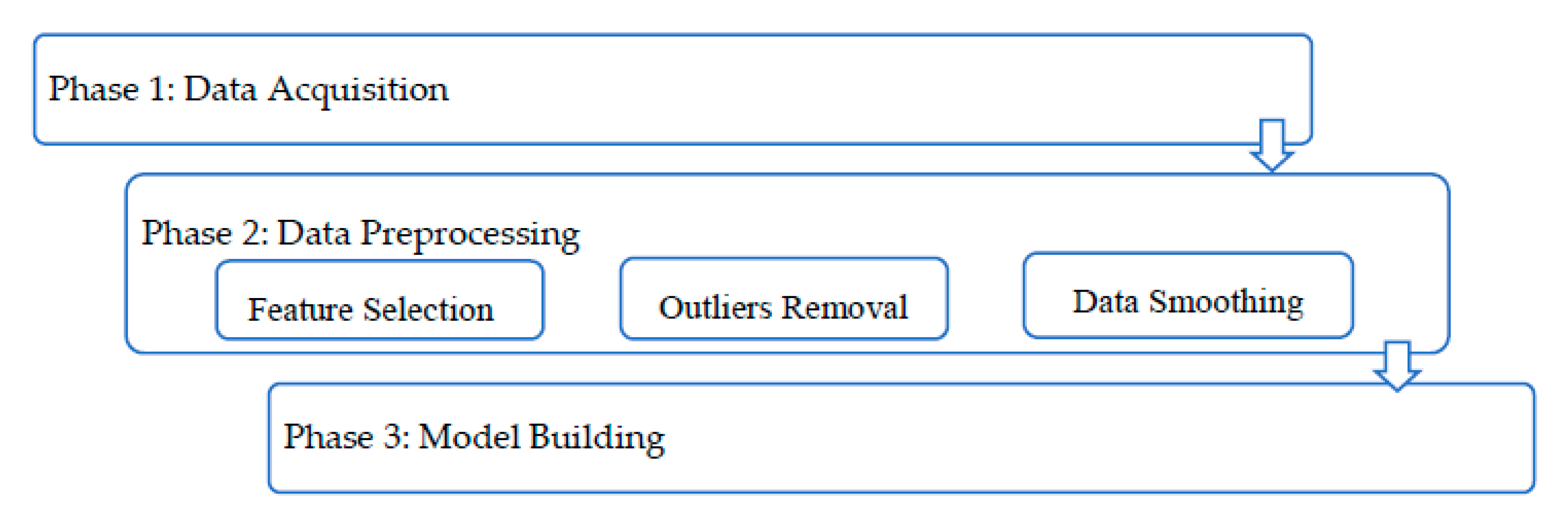
Figure 1.
Different phases and processing steps executed in the different edge of the network.
Figure 1.
Different phases and processing steps executed in the different edge of the network.
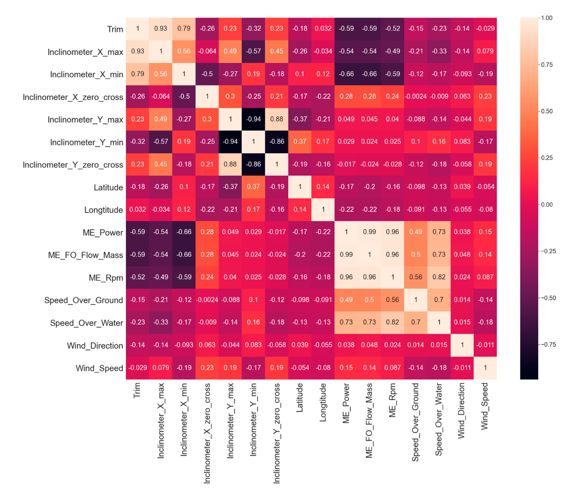
Figure 2.
A correlation heatmap (Pearson correlation) of the remaining selected features.
Figure 2.
A correlation heatmap (Pearson correlation) of the remaining selected features.
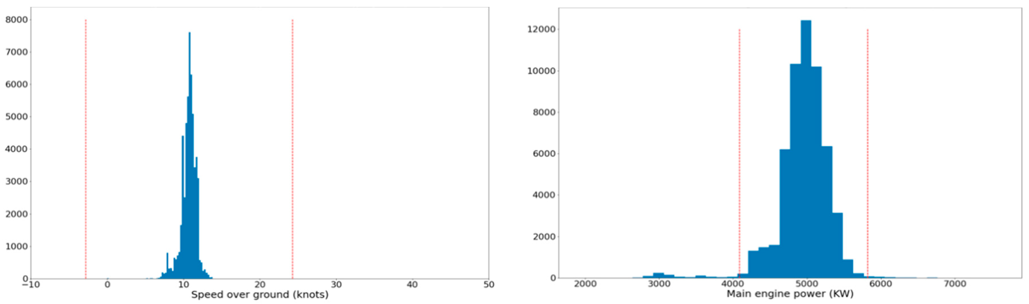
Figure 3.
Left: Histogram of the speed over ground for rpm values in the range (50,60). Right: Histogram of the power generated by the main engine for rpm values in the same range.
Figure 3.
Left: Histogram of the speed over ground for rpm values in the range (50,60). Right: Histogram of the power generated by the main engine for rpm values in the same range.
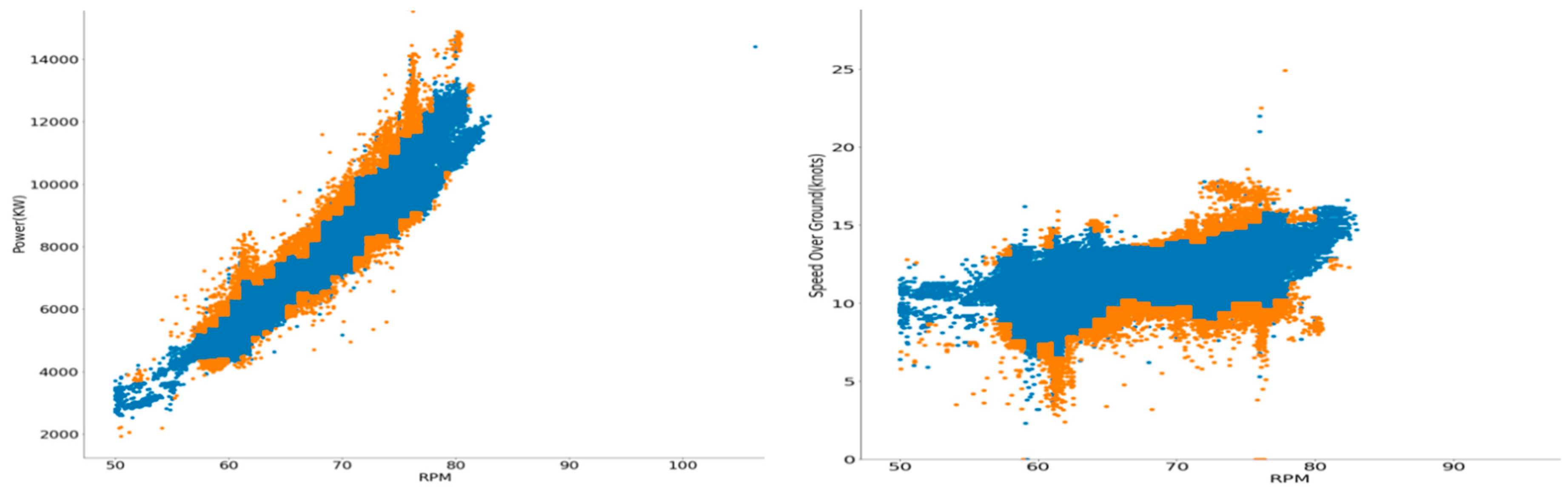
Figure 4.
Outlier removal with respect to main engine rpm; the left diagram corresponds to the power feature, and the right one to the speed over ground feature. Samples to be removed appear in orange, and the remainder of the data points appear in blue.
Figure 4.
Outlier removal with respect to main engine rpm; the left diagram corresponds to the power feature, and the right one to the speed over ground feature. Samples to be removed appear in orange, and the remainder of the data points appear in blue.
Figure 5.
The standard deviation of Main Engine power relative to the averaging time window.
Figure 5.
The standard deviation of Main Engine power relative to the averaging time window.
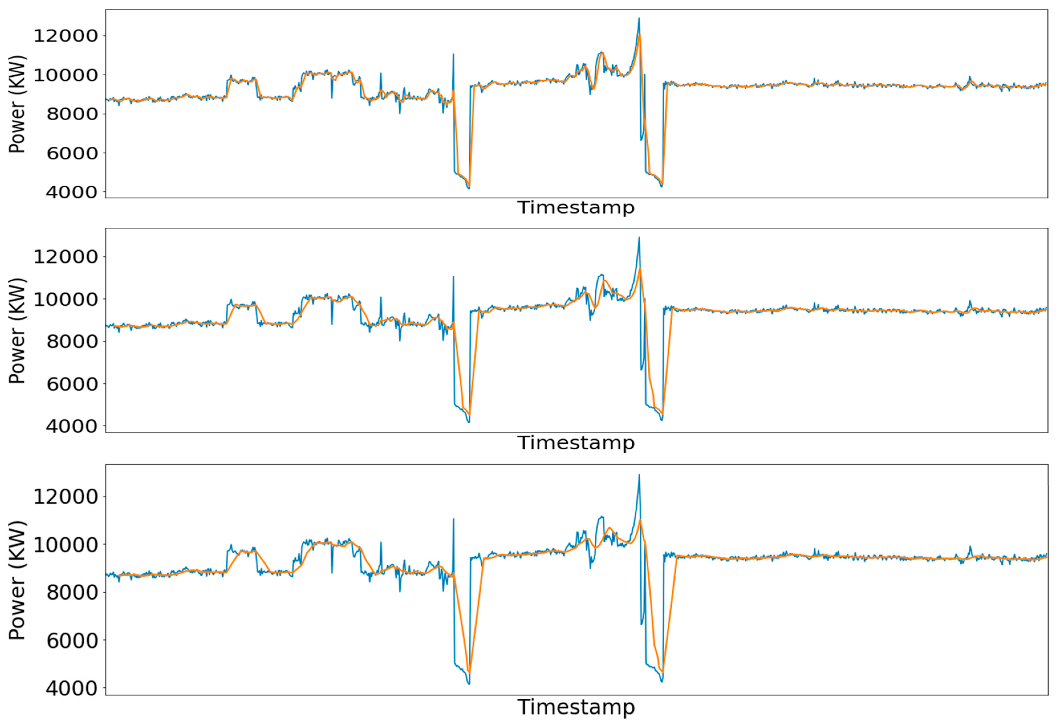
Figure 6.
Real (blue line) vs smoothed (red line) signal for a 5-min (up), 10-min (middle), and 15-min (down) averaging window.
Figure 6.
Real (blue line) vs smoothed (red line) signal for a 5-min (up), 10-min (middle), and 15-min (down) averaging window.
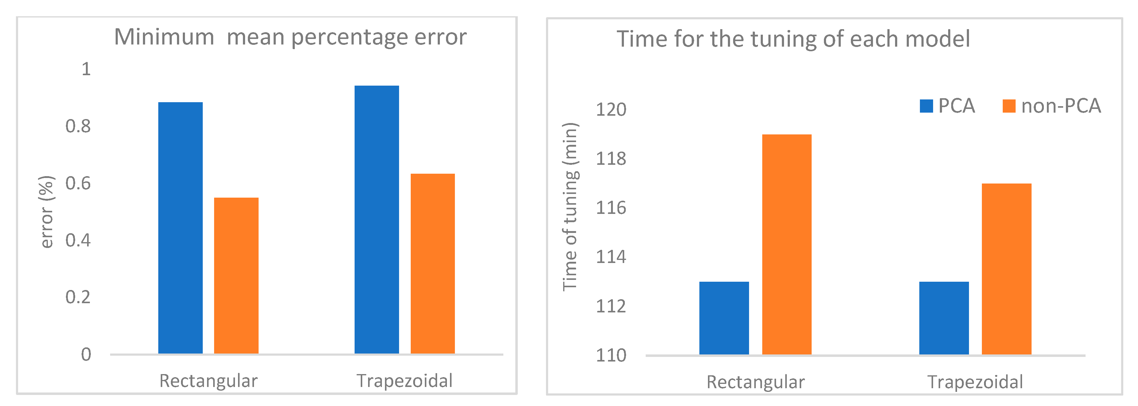
Figure 7.
Left: Comparison of the models concerning the mean percentage error each one achieved on the test set. Right: Comparison of the models concerning the time required for the hyperparameter tuning procedure.
Figure 7.
Left: Comparison of the models concerning the mean percentage error each one achieved on the test set. Right: Comparison of the models concerning the time required for the hyperparameter tuning procedure.
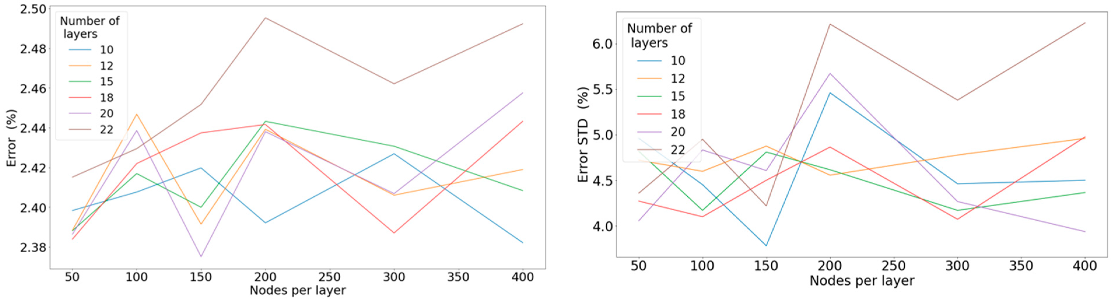
Figure 8.
Left: Mean percentage error concerning the number of nodes per layer for a different number of hidden layers when applying the linear activation function. Right: Standard deviation of the percentage error concerning the number of nodes per layer for a different number of hidden layers when applying the linear activation function.
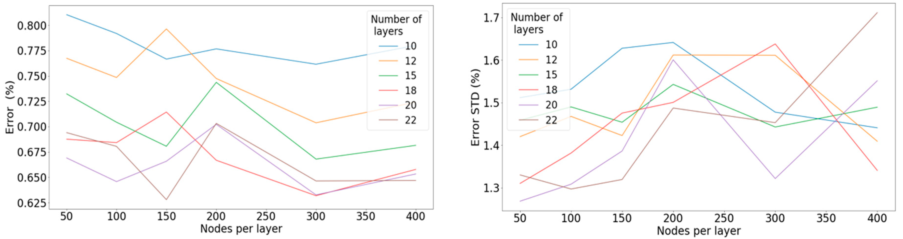
Figure 9.
Left: Mean percentage error concerning the number of nodes per layer for a different number of hidden layers when applying the ReLU activation function. Right: Standard deviation of the percentage error concerning the number of nodes per layer for a different number of hidden layers when applying the ReLU activation function.
Figure 10.
Learning-rate order of magnitude and its effect on the model performance.
Figure 10.
Learning-rate order of magnitude and its effect on the model performance.
Figure 11.
Left: Mean percentage error concerning the learning rate of the optimizer. Right: Standard deviation of the percentage error concerning the learning rate of the optimizer.
Figure 11.
Left: Mean percentage error concerning the learning rate of the optimizer. Right: Standard deviation of the percentage error concerning the learning rate of the optimizer.
Figure 12.
Left: Mean percentage error concerning the batch size. Right: Standard deviation of the percentage error concerning the batch size.
Figure 12.
Left: Mean percentage error concerning the batch size. Right: Standard deviation of the percentage error concerning the batch size.
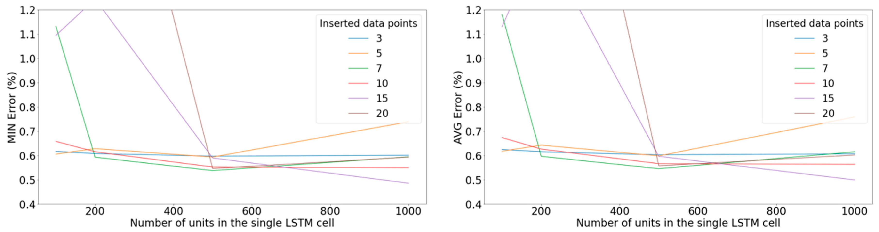
Figure 13.
Left: Minimum error on the validation set with respect to the number of units in the LSTM cell for various windows of inputted data points when applying the ReLU activation function. Right: Average error on the validation set among the 10 best-performing epochs with respect to the number of units in the LSTM cell for various windows of inputted data points when applying the ReLU activation function.
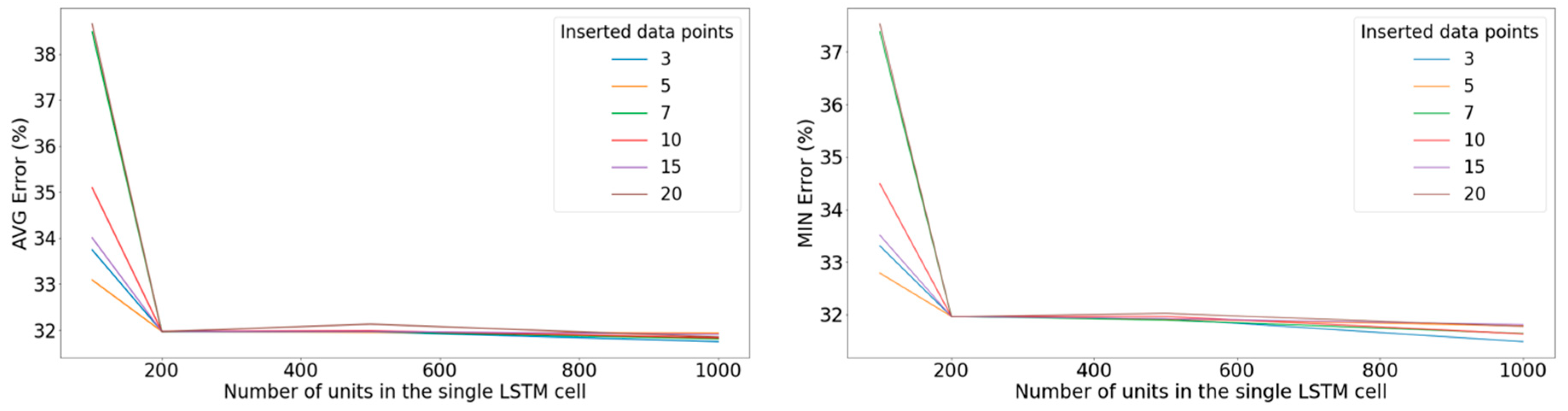
Figure 14.
Left: Minimum error on the validation set with respect to the number of units in the LSTM cell for various windows of inputted data points when applying the sigmoid activation function. Right: Average error on the validation set among the 10 best-performing epochs with respect to the number of units in the LSTM cell for various windows of inputted data points when applying the sigmoid activation function.
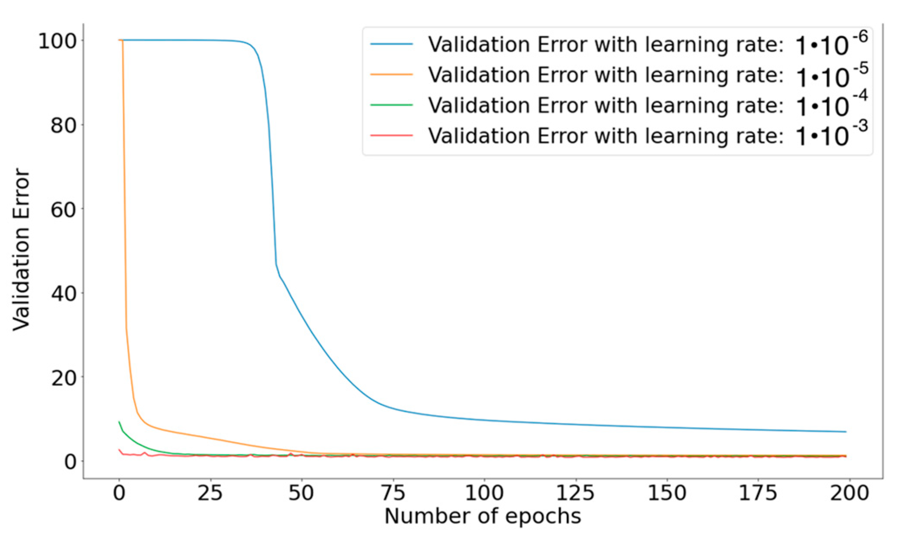
Figure 15.
Effect of the order of magnitude of the learning rate on the performance of the model.
Figure 15.
Effect of the order of magnitude of the learning rate on the performance of the model.
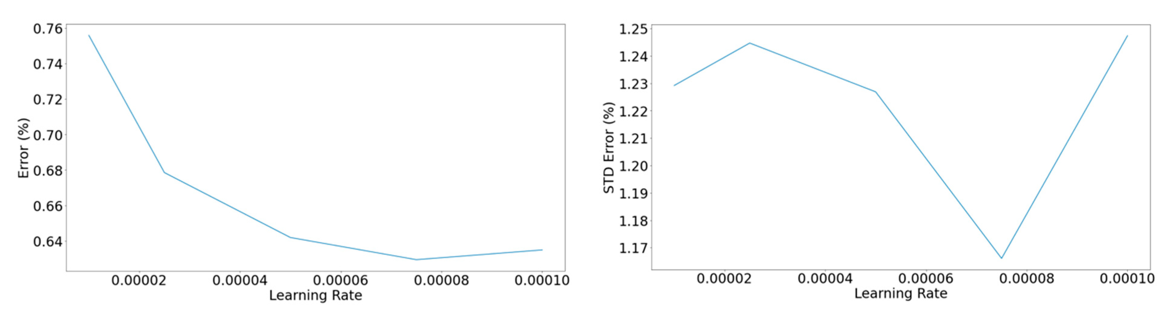
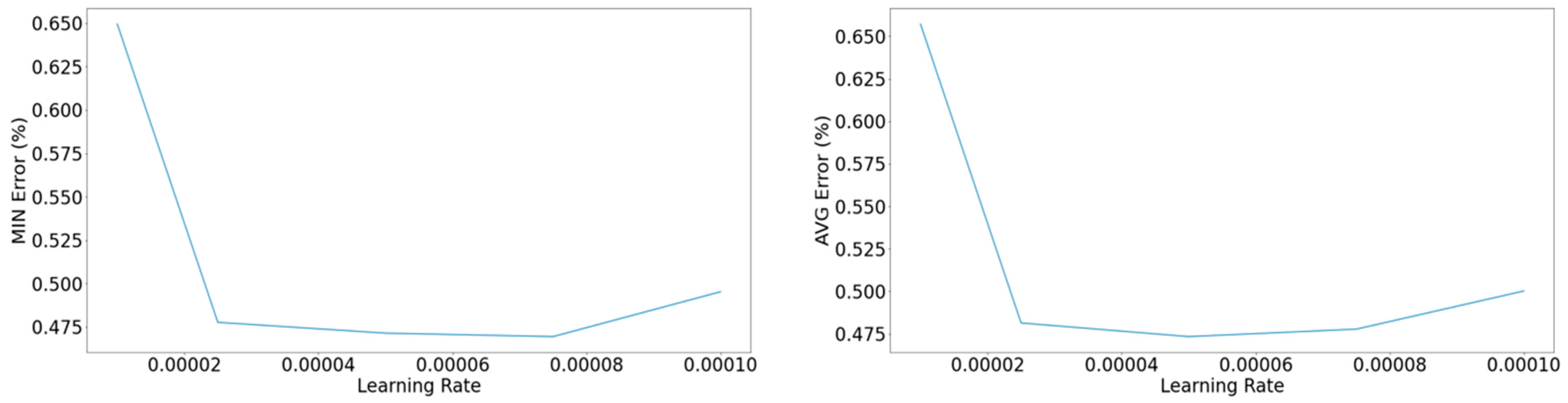
Figure 16.
Left: Minimum error on the validation set concerning the learning rate. Right: Average among the 10 epochs with the lower yielded error concerning the learning rate.
Figure 16.
Left: Minimum error on the validation set concerning the learning rate. Right: Average among the 10 epochs with the lower yielded error concerning the learning rate.
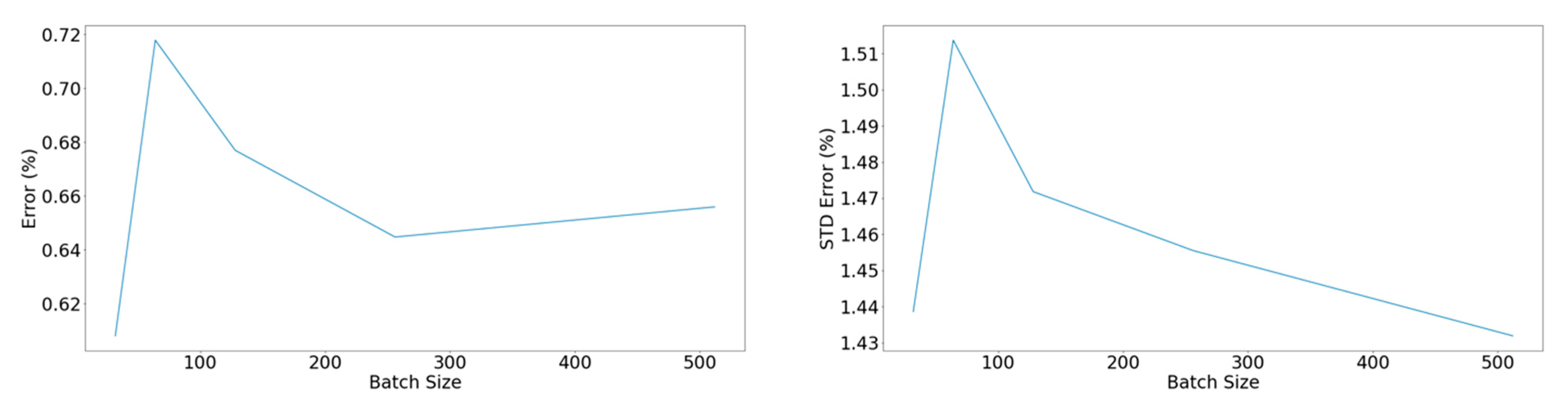
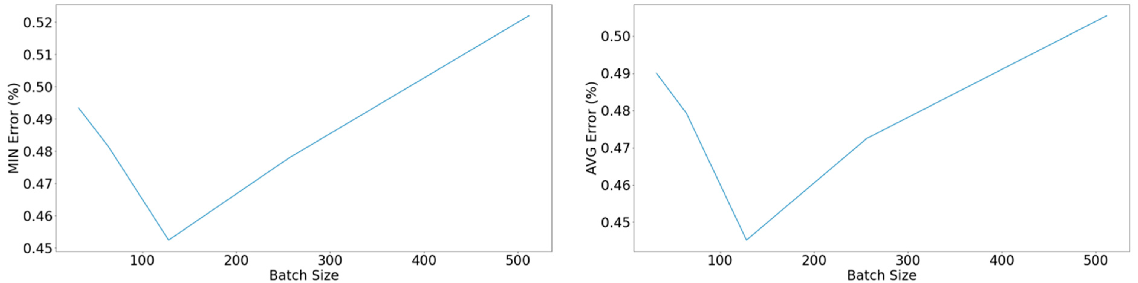
Figure 17.
Left: Minimum error of the validation set concerning the batch size. Right: Average among the 10 epochs with the lower yielded error concerning the batch size.
Figure 17.
Left: Minimum error of the validation set concerning the batch size. Right: Average among the 10 epochs with the lower yielded error concerning the batch size.
Figure 18.
Measured values of the shaft power and respective estimated ones using ANN.
Figure 18.
Measured values of the shaft power and respective estimated ones using ANN.
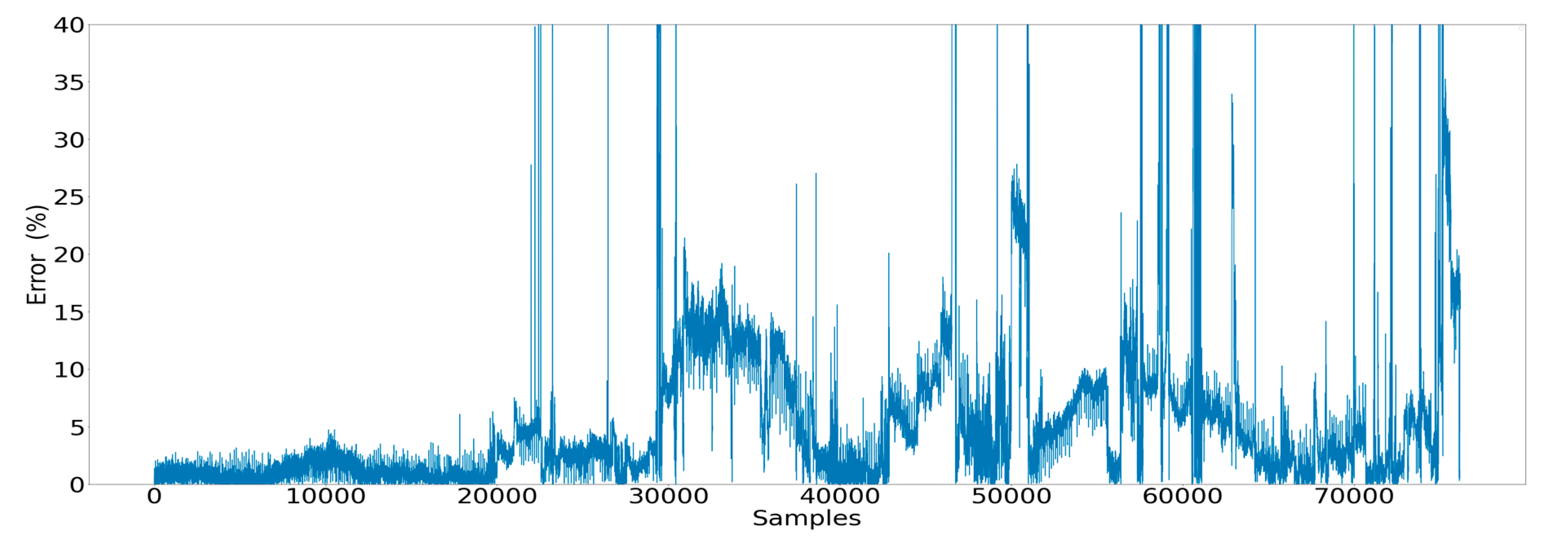
Figure 19.
Error observed for each data point estimated by the ANN model.
Figure 19.
Error observed for each data point estimated by the ANN model.
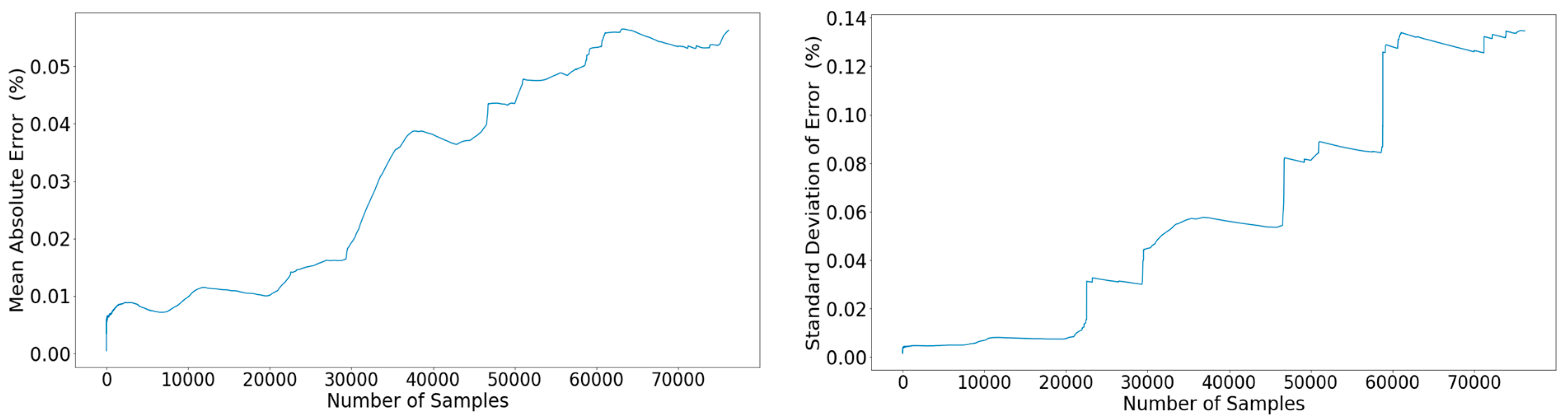
Figure 20.
Left: Propagation of the mean percentage error across the out-of-sample subset. Right: Propagation of the standard deviation of the error across the out-of-sample subset.
Figure 20.
Left: Propagation of the mean percentage error across the out-of-sample subset. Right: Propagation of the standard deviation of the error across the out-of-sample subset.
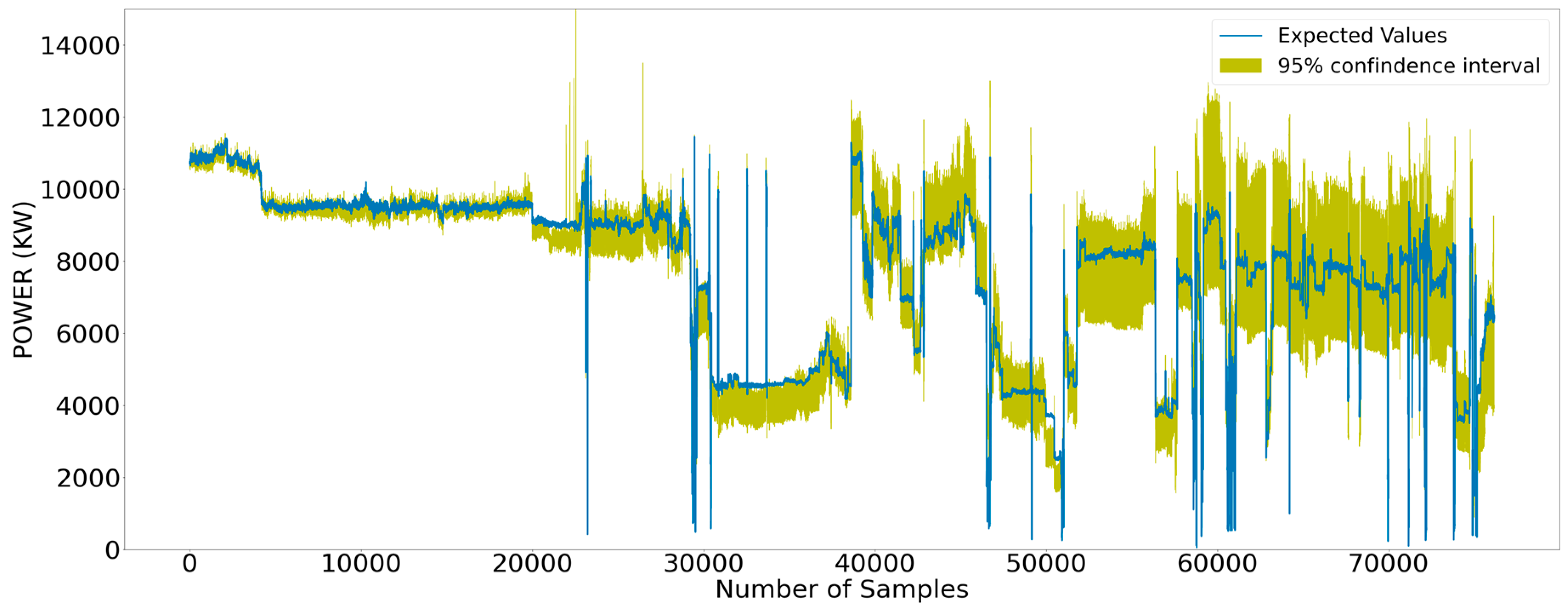
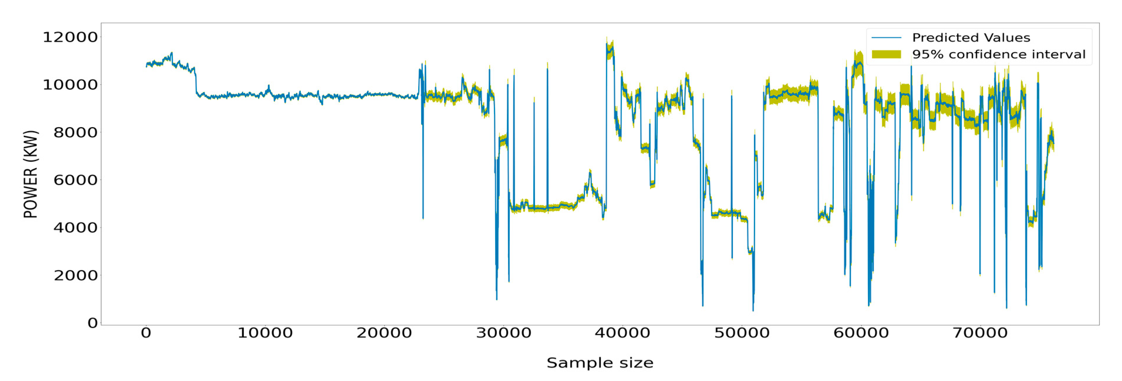
Figure 21.
Measured values surrounded by the respective 95% confidence interval that stemmed from the estimated values.
Figure 21.
Measured values surrounded by the respective 95% confidence interval that stemmed from the estimated values.
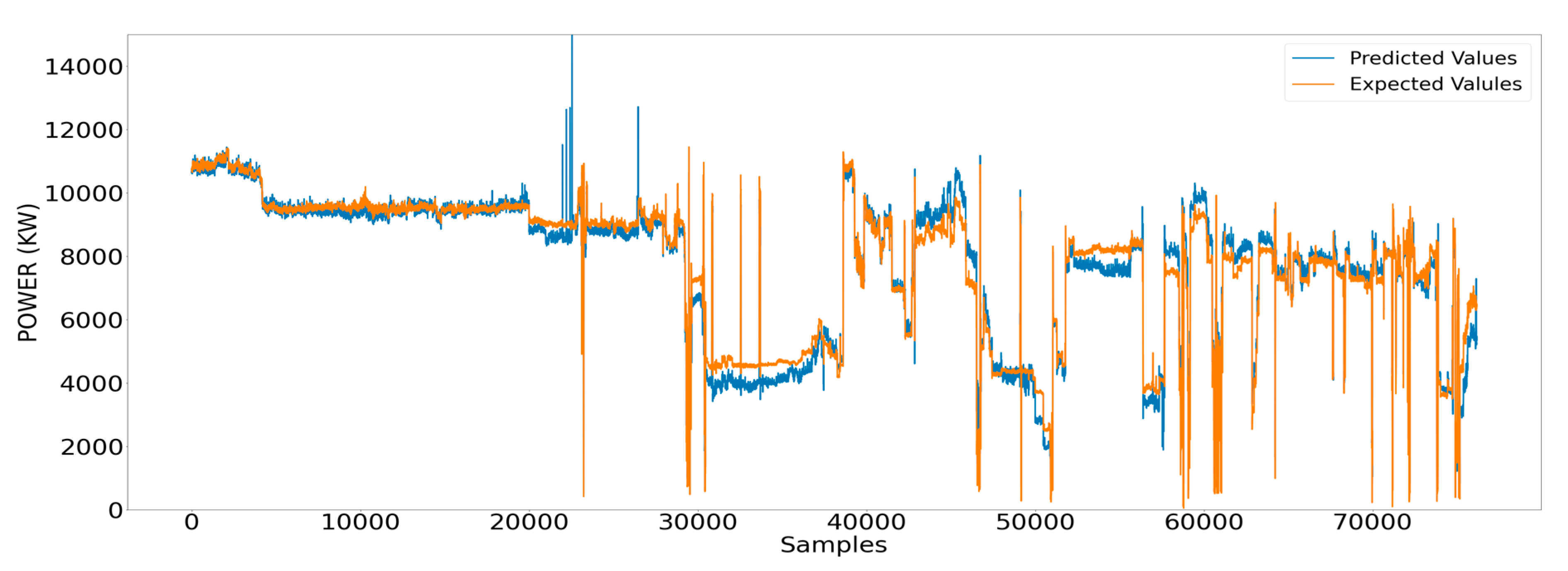
Figure 22.
Measured values of the shaft power and respective estimated ones using RNN models.
Figure 22.
Measured values of the shaft power and respective estimated ones using RNN models.
Figure 23.
Error observed for each data point estimated by the RNN models.
Figure 23.
Error observed for each data point estimated by the RNN models.
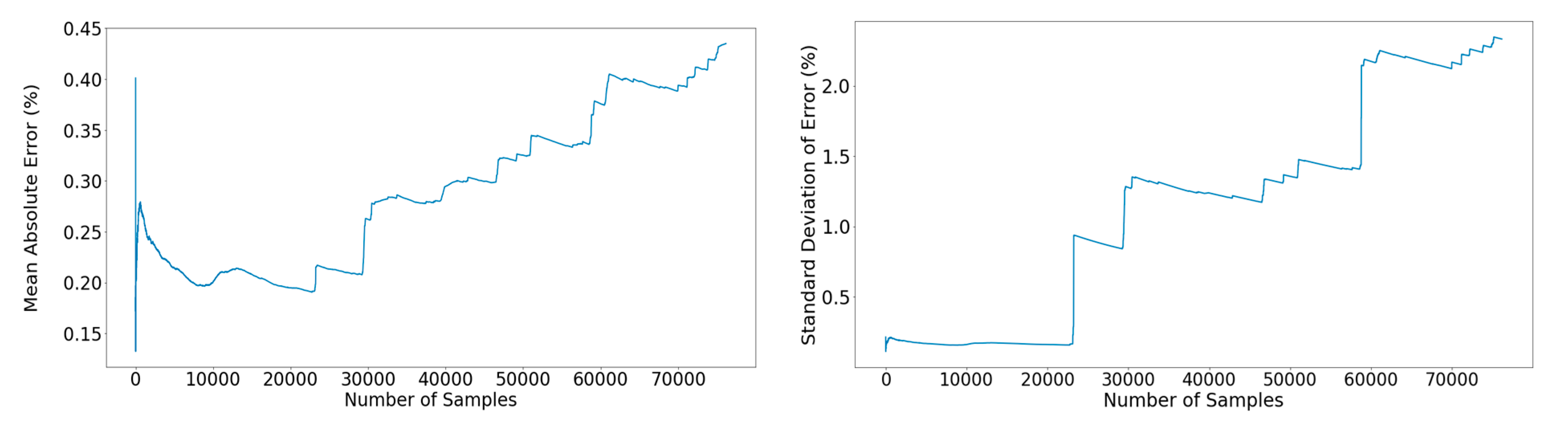
Figure 24.
Left: Propagation of the mean percentage error across the out-of-sample subset. Right: Propagation of the standard deviation of the error across the out-of-sample subset.
Figure 24.
Left: Propagation of the mean percentage error across the out-of-sample subset. Right: Propagation of the standard deviation of the error across the out-of-sample subset.
Figure 25.
Measured values of the power generated by the main engine surrounded by the respective 95% confidence interval that stemmed from the estimated values from the RNN models.
Figure 25.
Measured values of the power generated by the main engine surrounded by the respective 95% confidence interval that stemmed from the estimated values from the RNN models.
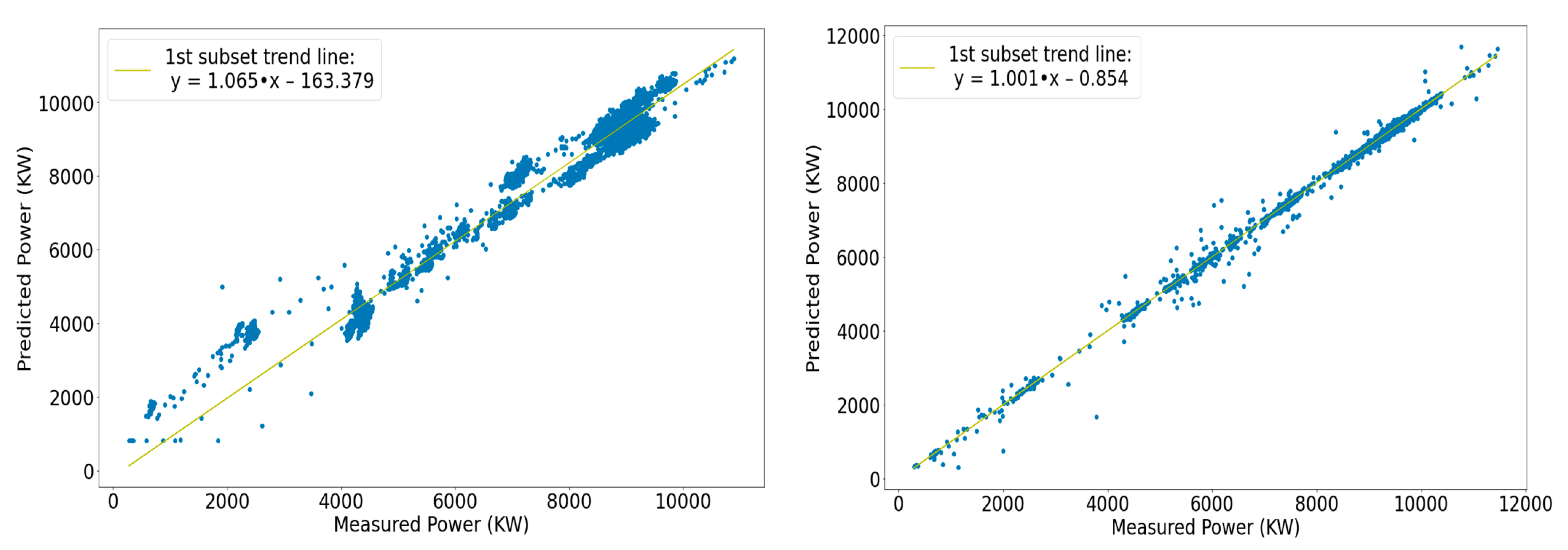
Figure 26.
Left: Scatter plot and optimal-fit line of the first segment of the FFNN model. Right: Scatter plot and optimal-fit line of the first segment of the RNN model.
Figure 26.
Left: Scatter plot and optimal-fit line of the first segment of the FFNN model. Right: Scatter plot and optimal-fit line of the first segment of the RNN model.
Figure 27.
Left: Optimal-fit lines for all segments of the FFNN model. Right: Optimal-fit line for all segments of the RNN model.
Figure 27.
Left: Optimal-fit lines for all segments of the FFNN model. Right: Optimal-fit line for all segments of the RNN model.
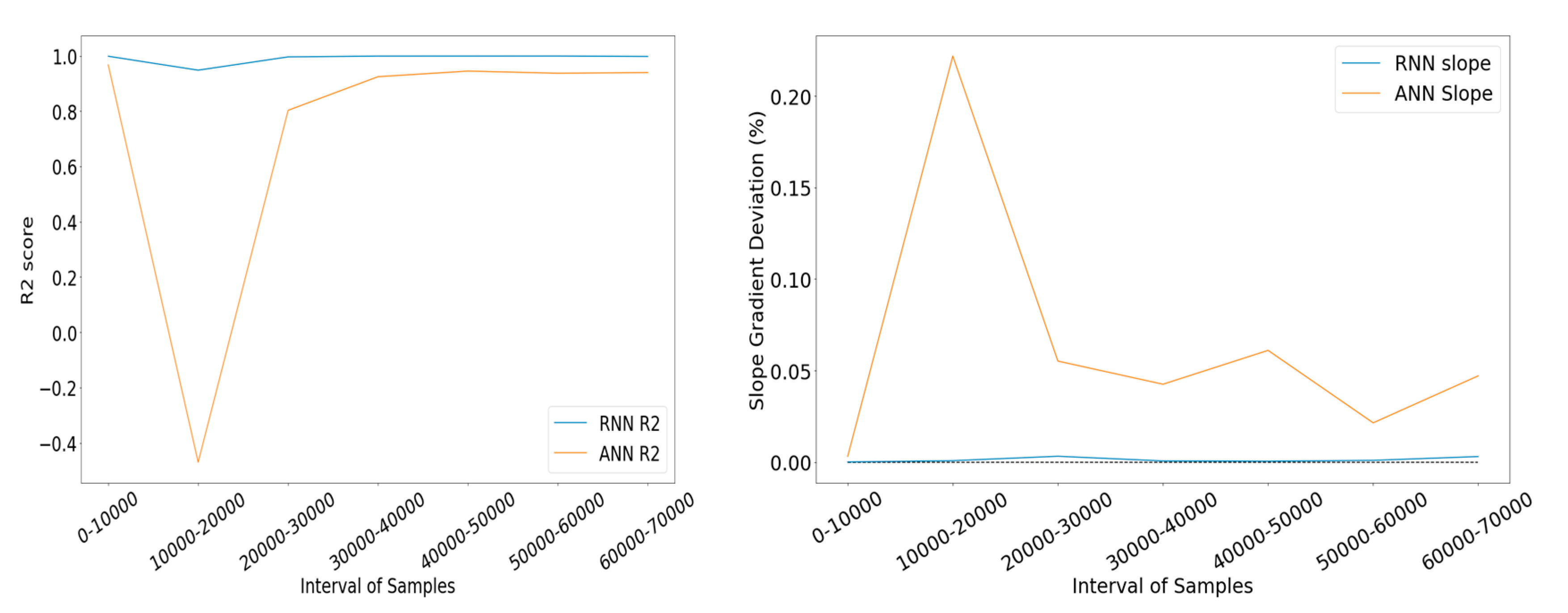
Figure 28.
Left: R2 score comparison between the types of networks. Right: Slope deviation comparison between the types of networks.
Figure 28.
Left: R2 score comparison between the types of networks. Right: Slope deviation comparison between the types of networks.
Figure 29.
Detecting the anomaly of degradation of the ship through the power increase deviation indicator.
Figure 29.
Detecting the anomaly of degradation of the ship through the power increase deviation indicator.
Table 1.
Ship’s Particulars.
Table 1.
Ship’s Particulars.
| Parameter | Value |
|---|
| Length | 264.00 (m) |
| Breadth (molded) | 50.00 (m) |
| Depth (molded) | 23.10 (m) |
| Engine’s MCR | 18,666 (kW) @ 91 RPM |
Table 2.
Collected parameters.
Table 2.
Collected parameters.
| Signal Source | Parameters |
|---|
| Navigational parameters | GPS, speed log, gyro compass, rudder angle, echo sounder, anemometer, inclinometer (pitching–rolling), drafts, weather data |
| Main engine (ME) | Torquemeter (shaft RPM, torque, power), ME fuel rack position %, ME FO pressure, ME scavenge air pressure, ME T/C RPM |
| Fuel-oil (FO) monitoring | ME FO consumption, diesel generator (DG) FO consumption |
| Alarm monitoring system | Indicative: DGs’ lube oil (LO) inlet pressure, cylinders’ exhaust gas outlet temperature, turbocharger (TC) LO pressure, TC inlet gas temperature, TC inlet gas temperature |
Table 3.
Initial selection of secondary hyperparameters.
Table 3.
Initial selection of secondary hyperparameters.
| Parameter | Value |
|---|
| Dropout rate | 0 |
| Kernel weight initializer | Uniform |
| Number of epochs | 250 |
Table 4.
Hyperparameters examination grid.
Table 4.
Hyperparameters examination grid.
| Parameter | Value |
|---|
| Number of layers | (10, 12, 15, 18, 20, 22) |
| Network’s width | (50, 100, 150, 200, 300, 400) |
| Activation function | (ReLU, Linear) |
Table 5.
Finalized configuration of the hyperparameters for the power-predicting model.
Table 5.
Finalized configuration of the hyperparameters for the power-predicting model.
| Parameter | Value |
|---|
| Learning rate | 2.5 × 10⁻⁴ |
| Number of layers | 20 |
| Maximum number of nodes per layer | 400 |
| Batch size | 128 |
| Epochs | 200 |
| Activation function | ReLU |
| Kernel initializer | Uniform |
| Dropout rate | 0 |
Table 6.
Values of secondary less-significant hyperparameters.
Table 6.
Values of secondary less-significant hyperparameters.
| Parameter | Value |
|---|
| Epochs | 200 |
| Dropout rate | 0 |
| Number of features inserted | 1 |
| Number of LSTM cells | 1 |
Table 7.
Hyperparameter tuning values.
Table 7.
Hyperparameter tuning values.
| Parameter | Value |
|---|
| Number of LSTM units in LSTM cell | (100, 200, 500, 1000) |
| Window of inserted data into the cell | (3, 5, 7, 10, 15, 20) |
| Activation function | ReLU, Sigmoid |
Table 8.
Finalized values of hyperparameters defining the LSTM power-predicting network.
Table 8.
Finalized values of hyperparameters defining the LSTM power-predicting network.
| Parameter | Value |
|---|
| Learning rate | 5 × 10⁻⁴ |
| Number of inputted samples | 15 |
| Number of units in LSTM cell | 1000 |
| Batch size | 128 |
| Epochs | 200 |
| Activation function | ReLU |
| Features inserted | 1 |
| Dropout rate | 0 |
Table 9.
Performance comparison of the two types of networks (mean error–percentage error).
Table 9.
Performance comparison of the two types of networks (mean error–percentage error).
| Parameter | FFNN | RNN |
|---|
| Power | 7 | 0.58 |
| Fuel Oil Consumption * | 5.8 | 0.58 |
Table 10.
Comparison of the training duration and the time * required for each network type to complete.
Table 10.
Comparison of the training duration and the time * required for each network type to complete.
| Parameter | FFNN | RNN |
|---|
| Training duration (min) | 16.67 | 57 |
| Time required for predictions (min) | 0.4 | 36 |


 ,
, 


