1. Introduction
It has been demonstrated, both experimentally [
1,
2,
3,
4,
5,
6] and theoretically [
6,
7,
8,
9,
10,
11], that in a three-dimensional (3D) oceanic waveguide, the horizontal refraction of the sound waves can be non-negligible. The manifestations of horizontal refraction are various and have been extensively studied for a few decades, for which the readers are referred to a special issue of papers on 3D underwater acoustics [
12] and the references therein. In this study, we put the emphasis on the horizontal multipath effect in wedge-like environments, in an attempt to diminish the error caused by the latter in the process of source bearing estimation. According to the simulations of the acoustic fields in a wedge, as well as the theory of ‘vertical mode, horizontal ray’, the received signal for each normal mode may contain an extra arrival (referred to as horizontally refracted arrival), in addition to a direct arrival, due to horizontal refraction [
5]. As confirmed in acoustic measurements off the Florida coast [
13], the received signals were composed of two distinct arrivals, i.e., a direct arrival and a horizontally refracted arrival, with the refracted path arriving as much as 30° inshore of the direct path. Previously, a similar phenomenon was also observed in the East Australian Continental slope, where bearing shifts deduced from beamformed data showed changes of tens of degrees in only half an hour [
1]. Since the source bearing is usually estimated as the arrival angle of the received signal, apparently the horizontally refracted path can cause a significant error in the estimation. Thus, it is natural to believe that the accuracy of bearing estimation can be improved by filtering out the horizontally-refracted path in the received signal. Meanwhile, it has been quantitatively demonstrated that the lower modes manifest less horizontal refraction than the higher modes in a coastal area [
14]. Thus, this paper exploits the feasibility of bearing estimation in a wedge by using the direct arrival for the lowest mode instead of the full signal. First, time-warping transform, which has been successfully employed to separate normal modes in horizontally stratified waveguides [
15,
16] and a weakly range-dependent waveguide [
17], is performed on the received signal. Second, the direct arrival component of the lowest mode is retained, while the rest of the signal is filtered out. Third, the bearing of the source is estimated with beamforming technology [
18]. Notice that it was also suggested by Petrov et al. [
14] that the first mode be used for solving long-range navigation problems in shallow water, because it is not only less affected by the horizontal refraction, but also less affected by attenuation.
The rest of the paper is organized as follows: In
Section 2, the images method for the wedge waveguide is briefly discussed, and an improved method for source bearing estimation in a 3D waveguide is presented, as a combination of the normal-mode separation technique and the conventional beamforming technique. In
Section 3, the performance of the improved method is tested in the case of a pulse signal in a wedge. Conclusions are given in
Section 4.
2. Theory
Here we consider the problem of acoustic propagation in a 3D wedge, which is a typical geometry in coastal areas. The acoustic field in the wedge, in the case of a harmonic source, can be obtained analytically using the method of source images [
8,
19]:
where
pnb,l denotes the field contributed by the source image
Snb,l, which can be written in the form of the plane wave decomposition:
Here
ns is the number of surface reflections and the bottom reflection number is
nb. For each value of
nb there is quadruple source images indexed by
l = –1, –2, 1, 2, with the only exception
nb = 0, when there are only two images with
l = –1, 2.
R = (
xr,
yr,
zr) is the position of the receiver,
k = (
kx,
ky,
kz) is the wavenumber vector, with components
kx,
ky, and
kz in the
xr,
yr, and
zr directions, respectively.
V(
γb) is the bottom reflection coefficient for the incident angle
γb. The readers are referred to [
8,
20] for more details of the source images method.
In the case where the source generates a pulse signal
S(
t), with the frequency spectrum denoted as
S(
ω), the received signal at the point (
x,
y,
ω) can be synthesized via a Fourier transform of the frequency-domain solution:
From the perspective of the normal mode theory, the received signal can be regarded as a sum of a series over normal modes:
The signal
pm (
x,
y,
z,
t) for each individual mode can become much more separable after applying the warping transform to the full signal
p (
x,
y,
z,
t). The warping transform means replacing the time
t in the expression of
p (
x,
y,
z,
t) with the warping factor:
where
t′ refers to the warped time, and
t0 is the reference time, which can be determined empirically, without knowing the distance between the source and receiver or the sound speed.
The array output vector for the received signal versus the azimuth angle
θ can be expressed as:
where
P = [
p1 p2 … pN],
N is the number of the array element,
A(θ) = [1 e
ikdsinθ … e
i(N-1)kdsinθ] is the steering vector, and
d is the element spacing. The angle corresponding to the peak of the array output is the estimated bearing of the sound source.
3. Simulation and Analysis
The geometry of the 3D penetrable wedge is illustrated in
Figure 1. It consists of an isovelocity water layer, with the sound speed
cw = 1500 m/s and the density
ρw = 1.0 g/cm
3, and a homogeneous half-space sediment layer, with the sound speed
csed = 1700 m/s, the density
ρsed = 1.5 g/cm
3, and the attenuation α
sed = 0.5 dB/λ. There is no attenuation in the water layer. The depth of the water–sediment interface is given by:
where
x =
rcos
θ. The water depth decreases linearly from 200 m at
x = 0 to 0 m at
x = 4.0 km along the
θ = 0° azimuth (up-slope direction), increases linearly from 200 m at
x = 0 to 400 m at
x = –4.0 km along the
θ = 180° azimuth (down-slope direction), and remains invariant along the line
θ = 90° and 270° azimuths (across-slope directions), making a wedge apex of 2.86°. Two arrays, labeled L1 and L2, are located 80 m below the water surface. Both of them are parallel to the x-axis and comprised of 15 elements with a spacing of 15 m. The center element of L1 and L2 are located at point A1 and point A2, respectively, which are both in the vertical plane of
x = 0 with
yA1 = 16 km and
yA2 = 22 km. The corresponding center elements are referred to as hydrophone A1 and hydrophone A2, respectively.
The right panel of
Figure 1 shows the modal ray diagrams in the horizontal
xoy plane for each omnidirectional modal initialization. Mode 1 arrives at A1 from an azimuth angle of
φ0 = 1.8°, while arrives at A2 through two paths, with the direct path from
φ0 = 2.7° and the horizontally refracted path from
φ0 = 19.7°. Mode 2 arrives at A1 through two paths, with the direct path from
φ0 = 13.5° and the horizontally refracted path from
φ0 = 16.5°. Note that the signal of mode 2 does not arrive at A2, since A2 is in the shadow zone of mode 2, due to the horizontal refraction.
An omnidirectional point source is located at point
S = (
xs = 0,
ys = 0,
zs = 0), with the time signal as a four-period sine wave given by:
where ω
c = 2
πfc denotes the center frequency. Here we set
fc = 25 Hz. The signal has a 40 Hz bandwidth covering the band 5–45 Hz.
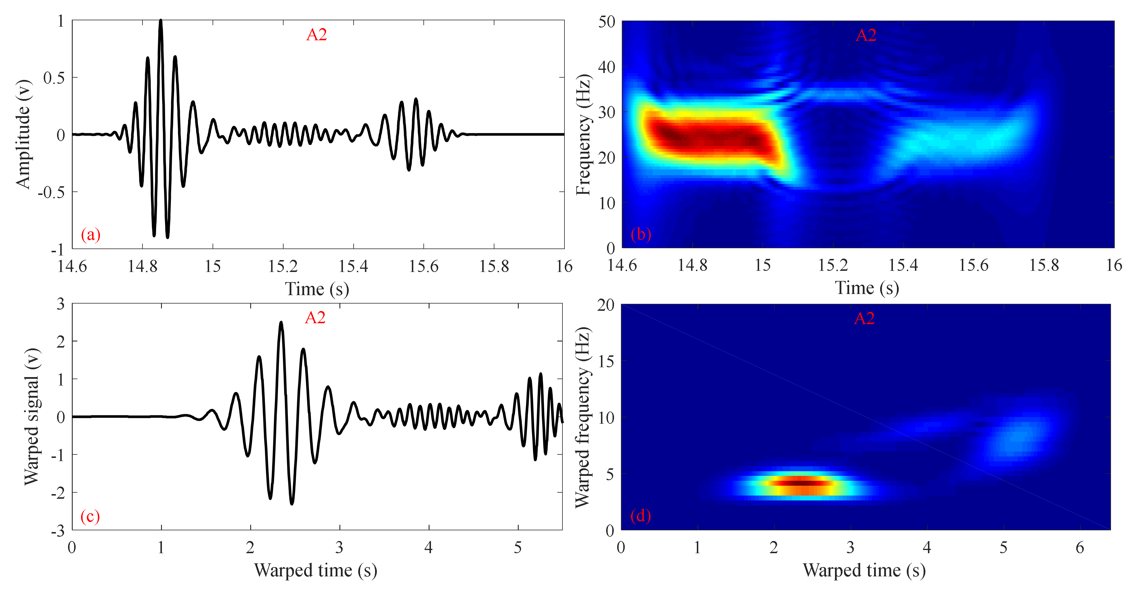
The signals received at A1 and A2 are shown in
Figure 2a and 3a. As we can see, the received signal at A1 consists of three distinct wave packets, with the first centered at
t = 10.81 s corresponding to the direct path of mode 1, the second centered at
t=11.15 s corresponding to the direct path mode 2, and the third as the very weak tail, corresponding to the refracted path mode 2. The received signal at A2 consists of two distinct wave packets, with the first one corresponding to the direct path of mode 1, and the second one (weaker) corresponding to the refracted path of mode 1.
Figure 2b and 3b present the short-time Fourier transform (STFT) of the received signals at A1 and A2, respectively. As we can see, the multiple arrivals of the signals are difficult to resolve with the modes in the time-frequency (TF) domain.
Here we employ time-warping transform, to separate multipath signals.
Figure 2c,d show the received signal at A1 after warping transform and the corresponding STFT. As we can see, mode 1 and mode 2 become more distinguishable in the TF domain, after warping transform. Retaining the selected mode, while filtering out the rest of the signal in the warped domain, and performing a reverse warping transform, we can obtain the signal for the selected mode in the original time domain.
Figure 3c,d show the receiving signal at A2, after warping transform and the corresponding STFT. Similarly to the A1 case, here the distinguishability between the direct and the refracted path of mode 1 is improved.
The signals for mode 1 and mode 2 at A1, after being separated, are shown in
Figure 4a,b and compared with the corresponding signals for the same modes calculated with a 2D propagation model, which ignores horizontal refraction. The difference between the 2D and 3D results reveals the effect of horizontal refraction. As can be observed, the difference between the 2D and 3D results for mode 2 is much more significant than for mode 1, indicating that higher modes are more significantly horizontally refracted than lower modes, which is consistent with the modal ray diagram shown in
Figure 1. In addition, it is interesting to note that the first wave packet of mode 1 seems almost unaffected by horizontal refraction; thus, this is probably the optimal part of the signal for estimating the true bearing of the source in a 3D waveguide.
The signals for the direct and refracted paths of mode 1 at A2, after being separated, are shown in
Figure 4c,d and compared with the mode 1 signal in the 2D case. As can be seen from
Figure 1, the direct path arrives nearly along the source–receiver line; however, the refracted path arrives from a much more shoreward direction, resulting in a longer path and higher bottom loss; in other words, leading to a higher lag and reduction in phase and amplitude, respectively, compared with the 2D result. Again, it is worth noting that the first wave packet of the direct path of mode 1 is almost unaffected by horizontal refraction, indicating the probability that this is the optimal part of the signal for estimating the true bearing of the source.
To summarize, the lower modes are less affected by the horizontal refraction than the higher modes, and the direct path of a certain mode is less affected by the horizontal refraction than the refracted path. Therefore, the direct path of the lowest mode is recommended, to be used to estimate the bearing of the source. Moreover, the first packet of the direct path of the lowest mode may be an even better choice (tested below).
The results of the bearing estimation, using the full signal, mode 1, mode 2, and the first packet signal of mode 1 (hereafter referred to as mode 1(I)) at A1 are compared in
Figure 5. The estimated bearing angles are listed in
Table 1. There are some deviations between the true and the estimated bearing angles, especially for mode 2, which is notably refracted in the horizontal direction, the deviation reaches 9.9°. Mode 1 is apparently less influenced by the horizontal refraction, and the absolute error of the estimation is only 2.3°. The estimation error when using the full signal lies between those for using solely mode 1 and mode 2. The estimation error can be further reduced by using the earliest packet of mode 1, with only a 1.5° estimation error.
The results of the bearing estimation using the full signal, the direct path of mode 1 (referred to as mode 1a), the refracted path of mode 1 (referred to as mode 1b), and the first packet of the direct path of mode 1 (referred to as mode 1a(I)) at A2 are compared in
Figure 6 and
Table 1. The estimation error in the case of using the refracted path (18.4°) is much larger than that of the direct path (2.0°), which is as expected. It is fortunate in this example that the refracted path contributes little to the entire field and, thus, has little influence on the estimation results when using the full signal; in other words, the estimation error when using the full signal (2.5°) is close to the estimation error when using only the direct path. This, nevertheless, does not mean in every case the refracted wave can be ignored. Last but not least, similarly to the case of A1, the estimation performance can be further improved by using the first packet of the direct path of mode 1, the absolute error of estimation is reduced to 1.4° by using mode 1a(I).
To investigate the influence of signal-to-noise ratio (SNR) on the source bearing estimation results, 100 independent Monte Carlo simulations were performed for a series of SNRs. The SNR is the ratio of signal energy to noise energy within the considered bandwidth. The root-mean-squared errors (
RMSE) for bearing estimation are given by
where
θn denotes the estimation result for the
nth Monte Carlo trial, and
θ0 is the true bearing. The simulation results are shown in
Figure 7. It is observed that under the investigated SNRs, the estimations using only the direct path of mode 1 (remember that for location A2, the direct path of mode 1 is identical to the entire mode 1, i.e., there is no refracted path of mode 1) always gave lower
RMSE than those using full modes, which was especially evident for the A1 site, where the
RMSE reach up to about 48.5 degrees, even under SNR = 5 dB for the estimations using full modes, while it quickly dropped to 5.2 and 3.25 degrees when using only the direct path mode 1 and its first packet, respectively. Note that the
RMSEs in the tested cases could not converge to 0, but could only converge to the values listed at the last column of
Table 1 when increasing the SNR to infinity. As observed from
Figure 7c,f, even for −10 dB SNR environments, our proposed method still exhibited acceptable estimation performance, confirming its anti-jamming capability.
4. Summary and Discussion
A method for underwater source-bearing estimation in a scenario incorporating horizontal refraction effects is presented. First, the full received signal is decomposed into a series of individual modes, by warping transformation and mode filtering. Second, the source bearing is estimated by performing beamforming of the lowest mode, i.e., the first mode or its direct path in cases where there exists a horizontally refracted path. It has been shown that in an ASA wedge, warping transformation has a good performance in separating different modes, as well as the direct path and refracted paths of the same mode. The error values for source-bearing estimation by beamforming of the full signal, the first mode, and the direct path of the first mode were compared for the same wedge case. The results show that the estimation error can be significantly reduced by beamforming with only the first mode, or the direct path of the first mode in cases where a horizontally refracted path of the first mode exists. For the cases with a series of different SNRs, the performance of our method in diminishing bearing error was also remarkable. Therefore, the idea of separating the direct path of the first mode in an ASA wedge for reducing bearing estimation was confirmed as feasible by our simulations. Although our mode filtering of the direct path of the first mode is not ideally clean, the error in bearing estimation can already be diminished.
Although this method was only validated in the ideal ASA wedge environment, and in a real coastal wedge the water sound speed profile and density can vary with depth and the seafloor does not have a constant sloping ratio, the received signals also consist of multiple modes, which are composed by a direct arrival and, possibly, a horizontally refracted arrival, which has been confirmed by both theoretical and experimental studies [
1,
5,
21]. Evidently, the propositions that lower modes refract less in the horizontal than higher modes, and that the direct paths refract less in the horizontal than the horizontally refracted paths still hold.
Another aspect that deserves further improvement is the technique of mode filtering, which is now limited to impulse signals, because of the use of warping transform as pre-processing here, which is recognized as being incapable of handling long-duration continuous signals, such as shipping noise. In future work, testing the performance of other mode filtering methods based on compressive sensing [
22] or variational Bayesian [
23] with a horizontal array would be warranted.


