Article

A Semi-Analytical Model for Studying Hydroelastic Behaviour of a Cylindrical Net Cage under Wave Action

1
School of Engineering and Built Environment, Griffith University, Gold Coast, QLD 4222, Australia
2
Cities Research Institute, Griffith University, Gold Coast, QLD 4222, Australia
3
School of Civil Engineering, The University of Queensland, St. Lucia, QLD 4072, Australia
*
Author to whom correspondence should be addressed.
J. Mar. Sci. Eng. 2021, 9(12), 1445; https://doi.org/10.3390/jmse9121445
Submission received: 28 November 2021 / Revised: 9 December 2021 / Accepted: 11 December 2021 / Published: 16 December 2021
(This article belongs to the Special Issue Hydrodynamics of Fish Cages and Floating Permeable Structures)

Abstract

:
In the present study, a semi-analytical model based on the small-amplitude wave theory is developed to describe the wave fields around a single gravity-type cylindrical open fish net cage. The cage may be submerged to different depths below the free-water surface. The fish cage net is modelled as a flexible porous membrane, and the deflection of the net chamber is expressed by the transverse vibration equation of strings. The velocity potential is expanded in the form of the Fourier–Bessel series and the unknown coefficients in these series are determined from matching the boundary conditions and the least squares method. The number of terms for the series solution to be used is determined from convergence studies. The model results exhibit significant hydroelastic characteristics of the net cages, including the distribution properties of wave surface, pressure drop at the net interface, structural deflection, and wave loading along the cage height. In addition, the relationships between wave forces on the net cage with hydrodynamic and structural parameters are also revealed. The findings presented herein should be useful to engineers who are designing fish cage systems.

1. Introduction

Fish farming not only provides an important protein supply for humans but also brings huge economic benefits. Average data from 2015 to 2017 indicates that fish products provide at least 20% of the animal protein intake of 3.3 billion people [1], and aquatic products accounted for about 46.4% of the food and agriculture production in 2017 [2]. In addition, the aquaculture industry of Australia is in a stage of rapid development and reached an annual output value of AUD 3.3 billion in 2020 [3]. In order to guarantee a stable output, the fishing cage system requires excellent reliability under environmental loads, such as waves and currents. Therefore, suitable modelling and studies on the dynamic response of the net cage to waves are crucial.
In many studies, the dynamic behaviour of fish cage nets is simulated by numerical models, for example, the bar element model in [4,5] or mass-spring model in [6,7], in which the hydrodynamic force on each element is estimated by the Morison equation or the screen-type method proposed by [8]. However, these models neglect the interferences of the structure and its motions on the flow field. For this reason, some researchers, e.g., Bi et al. [9] and Martin et al. [10], introduced computational fluid dynamics (CFD) techniques to achieve a fluid–structure interaction (FSI), but this requires tremendous computational time. In [10], it is reported that the simulation of a semisubmersible cage in irregular waves by FSI takes around 185 h for 300 s of simulation time on 64 cores (Intel Sandy Bridge) with 2.6 Ghz and 2 GB memory per core. This is not feasible to model a full-scale fish net cage in detail in engineering practice. If some characteristics of the wave passing through the net can be simplified and solved analytically, then the computational time can be reduced significantly.
Usually, in theoretical analysis that allows for interaction between net cage and waves, the wave field is described by the linear potential flow theory, and the fish cage net is modelled as a porous medium membrane. The porous wavemaker theory is proposed by Chwang [11] to analyse the water wave generated by the harmonic oscillation of a vertical porous barrier, where the porous flow is described by Darcy’s law. With the eigenfunction expansion and matching the boundary conditions, the particular solution of the velocity potential can be derived for the scattering issue of small-amplitude waves passing through permeable barriers in [12,13]. In terms of the interference effects among multiple rigid porous cylinders in waves, the scattering potential of each body in different local coordinates can be transformed by Graf’s addition theorem in [14,15]. Furthermore, if waves interact with flexible structures, the motion of the structure can be approximately described by the vibration equation of the continuum according to [16,17,18].
Recently, some studies have adopted the aforementioned theoretical approaches to analyse the interaction between waves and net cages. The transverse displacement of the circular cage is assumed to be governed by the vibration equation of the elastic beam in [19,20], and the deflection of the horizontal net plate can be described by the two-dimensional membrane vibration equation, which was introduced by [21]. Selvan et al. [22] extend the theory of [21] to the interference effect of multiple cages. Furthermore, Guo et al. [23] present a detailed review about the mathematical modelling of wave interaction with flexible net-type structures.
Moreover, a few researchers employed numerical techniques based on the linear potential flow theory to investigate the wave–structure interaction problems. The scaled boundary finite element model is applied to investigate the interaction mechanism between waves and pile groups with arbitrary spatial layouts and cross-sections in [24]. A hybrid method is adopted to evaluate the wave force acting on a cube net cage in [25], where the velocity potential of the far-field wave is expressed in the Fourier–Bessel series, and the ambient waves are solved by Green’s theorem, i.e., the boundary element method (BEM). In [26], the BEM and the Morison equation are combined to investigate the hydrodynamic characteristics of a semisubmersible aquaculture facility. The numerical and experimental comparisons in [25,26] both show acceptable agreement.
Based on the above literature review, several research gaps are identified. Firstly, when evaluating hydrodynamic loads with empirical models (Morrison equations or screen type methods), the wave field distribution induced by diffraction and radiation effects around the net cage has to be determined. Secondly, fish net cages may be designed with submerged capabilities to avoid strong surface waves. However, the above analytical models from [20,21,22] do not consider this scenario. Thirdly, for the net cage exposed to a wave field, knowledge about its hydroelastic behaviours is scarce. Therefore, it is essential to establish an analytical model to predict some key factors that determine the wave responses of fish net cages.
In the present study, the interactions between waves and submersible cylindrical fish net cage are approximated by a semi-analytical solution based on linear hydroelastic theory. The characteristics of the cage response to wave (free-water surface, pressure, hydrodynamic load, structural motion, etc.) are to be determined. This information is crucial for the design and application of fish cages. The linear model has advantages in the derivation of analytical solutions even if the boundary value problem is relatively complicated. The potential flow theory is also convenient for dealing with the domain with an infinite boundary, which means that an extremely large wave field is feasible to be analysed. The paper is arranged as follows: Section 2 presents the assumptions, modelling, governing equation, and boundary conditions for the wave–cage interaction problem. In Section 3, the method of solution for the governing equations and boundary value problems is elaborated. Section 4 presents the convergence studies and model validation. Section 5 presents the calculated results and explains the hydroelastic behaviour of the net cage under wave action. In Section 6, parametric studies are established to reveal the relationship between the wave force on the net cage and various hydrodynamic and structural parameters. Finally, brief conclusions are given in Section 7.

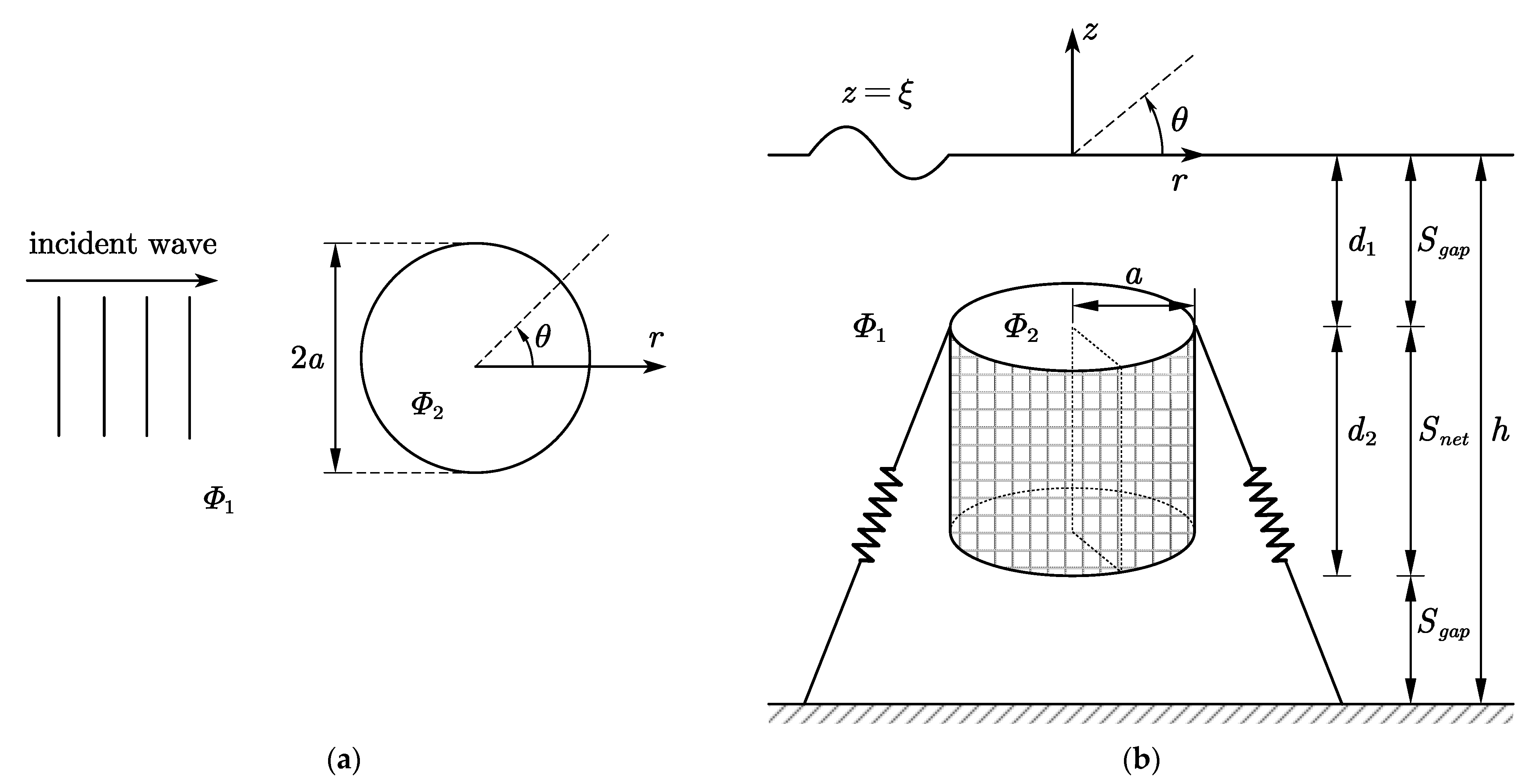
2. Problem Definition, Assumptions, Modelling, Governing Equation, and Boundary Conditions

In this study, a cylindrical net cage is considered as shown in Figure 1, and it is convenient to describe the physical problem in a cylindrical coordinate system (r, θ, z). A small-amplitude wave propagates along the direction of θ = 0 with a circular frequency ω and a wave height H. The mean water level is at z = 0, and the cage is submerged in a finite water depth of h. The central axis of the cage with a height of d2 is located at the position r = 0, and its top end can be submerged below the mean water level in d1. In addition, the top end is constrained by mooring systems at z = −d1, whilst the bottom end of z = −(d1 + d2) is free.
The flow domain may be divided into two zones: Region 1 (r > a, −h < z < 0) is the external region outside the net cage, while Region 2 (r < a, −h < z < 0) is the area within the circular net chamber. For the structural domain, the notations Snet and Sgap represent the net region of −(d1 + d2) ≤ zd1 and the gap portions of −d1 < z ≤ 0 ∪ −hz < −(d1 + d2), respectively.
The problem at hand is to determine the hydroelastic behaviour of the submerged cylindrical net cage under wave action.

2.1. Governing Equations

Assuming that the fluid is incompressible, irrotational, and inviscid, Φ1 and Φ2 represent the velocity potentials in Regions 1 and 2, respectively, and the velocity potential Φj (r, θ, z, t) (j = 1, 2) can be written as
Φ j = Re [ φ j ( r , θ , z ) e i ω t ] ,
where φj is the spatial component of the velocity potential, and it is governed by the Laplace equation in the cylindrical coordinate:
2 φ j r + 1 r φ j r + 1 r 2 2 φ j θ + 2 φ j z 2 = 0 .
In addition, φj can be represented as a superposition of the incident wave component φI and the scattered (diffraction and radiation) wave component φ j S , i.e.,
φ j = φ I + φ j S .

2.2. Boundary Conditions

At the free-water surface z = ξ, the linearised kinematic free surface (KFSBC) boundary condition satisfies
Φ j z = ξ t ,   at   z = 0 ,
and dynamic free surface boundary condition (DFSBC) is
ξ = 1 g Φ j t ,   at   z = 0 .
By combining Equation (4a,b), the boundary condition at the mean water level is
φ j z ω 2 g φ j = 0 ,   at   z = 0 ,
and the slip boundary condition on the seabed is given by
φ j z = 0 ,   at   z = h .
Furthermore, the scattered potential component φ j S satisfies the Sommerfeld radiation condition when r approaches infinity [27], i.e.,
lim r r ( φ 1 S r i k 0 φ 1 S ) = 0 ,
where k0 is the incident wavenumber.
As shown in Figure 2, the cage net is modelled as a porous membrane, so the penetrated flow through the net interface satisfies the linearised kinematic condition:
φ j r =   i σ ( φ 2 φ 1 ) i ω η c o s θ ,   at   r = a   and   z S net ,
in which η is the spatial component of the transverse deflection of the cage along the incident direction of the wave, and σ is the porous-effect parameter of the net that is expressed by an empirical formula given by Ito et al. [25]:
σ = ( 1   +   i σ i ) σ r
σ r = k 0 2 π × ( 27.73 / ε + 469.0 ) G 2 1 + ( 0.5510 0.01998 / ε ) G ,
where G is the opening ratio of the net, ε is the incident wave slope Hk0/2, and the imaginary part of σ represents the fluid inertia effect. A high Keulegan–Carpenter number indicates a minor fluid inertia effect compared to the fluid drag effect. In [7], for the net twine with a diameter of a few millimetres, its KC (Keulegan–Carpenter) number is 160 to 350 based on the laboratory tests, and the wave-induced inertia force is considered negligible compared to its drag force on the fish net. In the real sea condition, higher wave height and wave periods also mean a greater KC number. Currently, there is no appropriate formula of σi given for the cylindrical net cage; therefore, it is taken as 0 if there is no special explanation. Notably, the influence of σi is discussed in Section 6.
In addition, the continuity of the normal velocity and pressure of the flow at the interface between Regions 1 and 2 requires
φ 1 r = φ 2 r ,   at   r = a , h   <   z   <   0 ,
φ 1 = φ 2 ,   at   r = a   and   z S g a p .
On the other hand, it is assumed that the cross-section of the cage maintains its circular shape under wave action if the cage is imposed a high axial tension and has a small deformation relative to its overall size. Liu et al. [28] showed a deformed net cage simulated by the finite element method using truss elements, and it is observed that the cage approximately maintains a circular cross-section. Therefore, the transverse deflection of the cage is ζ = Re[η(z)e-iωt], and the transverse vibration equation of the string to describe the complex amplitude η is given by Mandal and Sahoo [21]:
d 2 η d z 2 + m s ω 2 Q η = a i ω ρ Q 0 2 π ( φ 1 φ 2 ) cos ( π θ ) d θ ,
in which Q is the axial uniform tensile force in the net, ms is the uniform mass of the net per unit length, and ρ is the water density. In [28], a comparison between the analytical model based on Equation (10) and the FEM simulation for the cylindrical net cage illustrates acceptable errors.
For the edge restraint condition of the net chamber, its top end is assumed to be constrained by the mooring systems according to [28], and there is no transverse traction at the bottom end, i.e.,
Q d η d z = k s η ,   at   z = d 1 ,
d η d z = 0 ,   at   z = ( d 1 + d 2 ) .
where ks is the spring constant of the mooring cables.

3. Method of Solutions

In view of the governing equation, Equation (2), and the boundary conditions, Equations (4c), (5), and (6), the solution of φ1 is sought in the form
φ 1 = φ I + φ 1 S ,
where
φ I = m = 0 i g H 2 ω cos h [ k 0 ( z + h ) ] cosh ( k 0 h ) μ m J m ( k 0 r ) cos ( m θ ) ,
μ m = { 1 ,               m = 0 2 i m ,       m > 0 ,
φ 1 S = m = 0 n = 0 A m n R m 1 ( k n r ) f n ( z ) cos ( m θ ) ,
R m 1 ( k n r ) = { H m ( k n r ) H m ( k n a ) ,     n = 0 K m ( k n r ) K m ( k n a ) ,     n > 0 ,
f n ( z ) = { cos h [ k n ( z + h ) ] cos h ( k n h ) ,     n = 0 cos [ k n ( z + h ) ] cos ( k n h ) ,     n > 0 .
Similarly, according to the governing equation, Equation (2), and the boundary conditions, Equations (4c) and (5), the general solution of φ2 is
φ 1 = φ I + φ 1 S ,
where
φ 2 S = m = 0 n = 0 B m n R m 2 ( k n r ) f n ( z ) cos ( m θ ) ,
R m 2 ( k n r ) = { J m ( k n r ) J m ( k n a ) ,     n = 0 I m ( k n r ) I m ( k n a ) ,     n > 0 .
kns are the real roots of the following dispersion relations:
{ ω 2 = g k n tanh ( k n h ) ,     n = 0 ω 2 = g k n tan ( k n h ) ,     n > 0   ,
and Amn and Bmn are the unknown constants, Jm is the first kind of Bessel function, Hm is the first kind of Hankel function, Im is the first kind of modified Bessel function, and Km is the second kind of modified Bessel function, where the subscript m is the order of the Bessel function.
By substituting Equations (12a–f) and (13a–c) into the boundary condition Equation (9a) and applying the orthogonality operation of cosh[kn(z + h)], cos(knh), n = 0, 1, 2 … over −hz ≤ 0 and cos(), m = 0, 1, 2 … over 0 ≤ θ ≤ 2π, the unknown constants in Equations (12d) and (13b) satisfy
A m n = B m n .
Therefore, one can write
Δ φ = φ 1 φ 2 = m = 0 n = 0 A m n X m n f n ( z ) cos ( m θ ) ,   at   r = a ,
where
X m n = R m 1 ( k n a ) R m 2 ( k n a ) .  
By substituting Equation (16a,b) into Equation (10) and noting the orthogonality of cos(), m = 0, 1, 2 … over 0 ≤ θ ≤ 2π, Equation (10) might be rewritten as
d 2 η d z 2 + α 1 η = α 2 n = 0 A 1 n X 1 n f n ( z ) ,
where
α 1 = m s ω 2 / Q   and   α 2 = π a i ω ρ / Q .
Therefore, the general solution for η(z) is
η ( z ) = κ = 1 2 C κ e q κ z + n = 0 A 1 n F n f n ( z ) ,
in which
F n = { α 2 X 1 n α 1 + k n 2 ,     n = 0 α 2 X 1 n α 1 k n 2 ,     n > 0 ,
and qκs are the roots of the characteristic equation of Equation (17a), and they are given by
q 1 = i ω m s / Q   and   q 2 = i ω m s / Q .
By substituting Equation (18a–c) into the boundary condition, Equation (11a,b), the constant Cκs are acquired through
{ κ = 1 2 C κ ( k s q Q ) e q κ d 1 + n = 0 A 1 n [ k s F n f n ( d 1 ) Q F n f n ( d 1 ) ] = 0 κ = 1 2 C κ q κ e q κ ( d 1 + d 2 ) + n = 0 A 1 n F n f n [ ( d 1 + d 2 ) ] = 0 .
For the net portion z∈Snet, substituting Equations (12a–f), (16a,b), and (18a–c) into Equation (7) and invoking the orthogonality of cos(mθ) again, one obtains,
when m ≠ 1,
n = 0 A m n k n f n ( z ) + i σ n = 0 A m n X m n f n ( z ) i g H k 0 2 ω cos h [ k 0 ( z + h ) ] cos h ( k 0 h ) μ m J m ( k 0 a ) = 0 ,
and when m = 1,
n = 0 A 1 n k n f n ( z ) + i σ n = 0 A 1 n X 1 n f n ( z ) + i ω n = 0 A 1 n F n f n ( z ) i g H k 0 2 ω cos h [ k 0 ( z + h ) ] cos h ( k 0 h ) μ m J m ( k 0 a ) + i ω j = 1 2 C κ e q κ z = 0 .
For the gap portion z∈Sgap, substituting Equation (16a) into Equation (9b) and using the orthogonality of cos() yields
n = 0 A m n X m n f n ( z ) = 0 .
As a result, a system of equations can be obtained from Equations (20a,b) and (21):
S m ( z ) = n = 0 A m n ϵ m n ( z ) + λ m ( z ) = 0 ,
where, when m ≠ 1,
ϵ m n ( z ) = { ( k n + i σ X m n ) f n ( z ) ,       z S n e t X m n f n ( z ) ,       z S g a p ,
λ m ( z ) = { i g H k 0 2 ω cos h [ k 0 ( z + h ) ] cos h ( k 0 h ) μ m J m ( k 0 a ) ,       z S n e t 0 ,       z S g a p ,
and when m = 1,
ϵ m n ( z ) = { ( k n + i σ X m n + i ω F n ) f n ( z ) ,       z S n e t X m n f n ( z ) ,       z S g a p ,
λ m ( z ) = { i g H k 0 2 ω cos h [ k 0 ( z + h ) ] cos h ( k 0 h ) μ m J m ( k 0 a ) + i ω j = 1 2 C κ e q κ z ,       z S n e t 0 ,       z S g a p .  
Truncating the infinite series after Nth terms in Equation (22a) yields
S m ( z ) = n = 0 N A m n ϵ m n ( z ) + λ m ( z ) = 0 .
By manipulating the least-squares approximation for Equation (23), one obtains
h 0 | S m ( z ) | 2 d z = m i n h 0 S m * S ( z ) A m n d z = 0 ,
and a system of equations about Amn is acquired by substituting Equation (23) into Equation (24):
n = 0 N A m n * Ψ m n , l = Ω m . l ,
where
Ψ m n , l = h 0 ϵ m n * ϵ m , l d z   and   Ω m , l = h 0 λ m * ϵ m , l d z ,
and m = 0, 1, 2, …, M; l = 0, 1, 2, …, N.
Therefore, Amn and Cκ are solved by combining Equations (19) and (25a,b), and the complex amplitude of the velocity potential φj is calculated from Equations (12a–f) and (13a–c).
Finally, in view of the linearised Bernoulli’s equation, the complex dynamic pressure p is
p j = ρ ( φ j e i ω t ) t ,
and the complex pressure difference acting on the net interface is defined as
Δ p = p 1 p 2 ,   at   r = a .
As a result, the complex function of the horizontal hydrodynamic force per unit length along the cage height is given by
f ( z ) = a 0 2 π Δ p cos ( π θ ) d θ = π a i ω ρ n = 0 N A 1 n X 1 n f n ( z ) e i ω t ,
and the wave force and the resulting overturning moment with respect to the top of the cage are
F = ( d 1 + d 2 ) d 1 f ( z ) d z   and   M o = ( d 1 + d 2 ) d 1 f ( z ) ( z + d 1 + d 2 2 ) d z .
Furthermore, according to the DFSBC, Equation (4b), the free-water surface elevation ξ is given by
ξ j = Re ( i ω φ j e i ω t g ) .

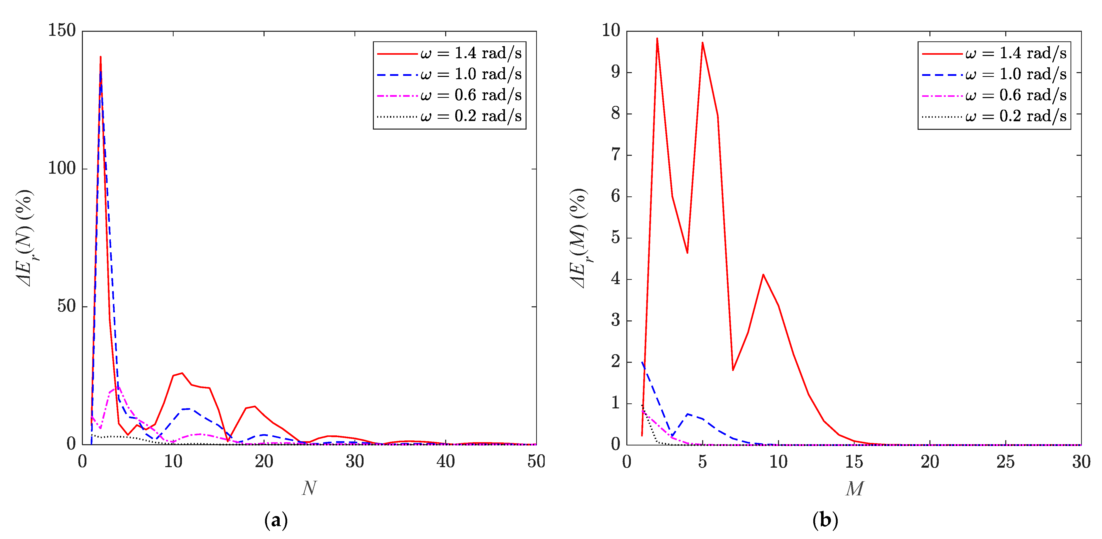
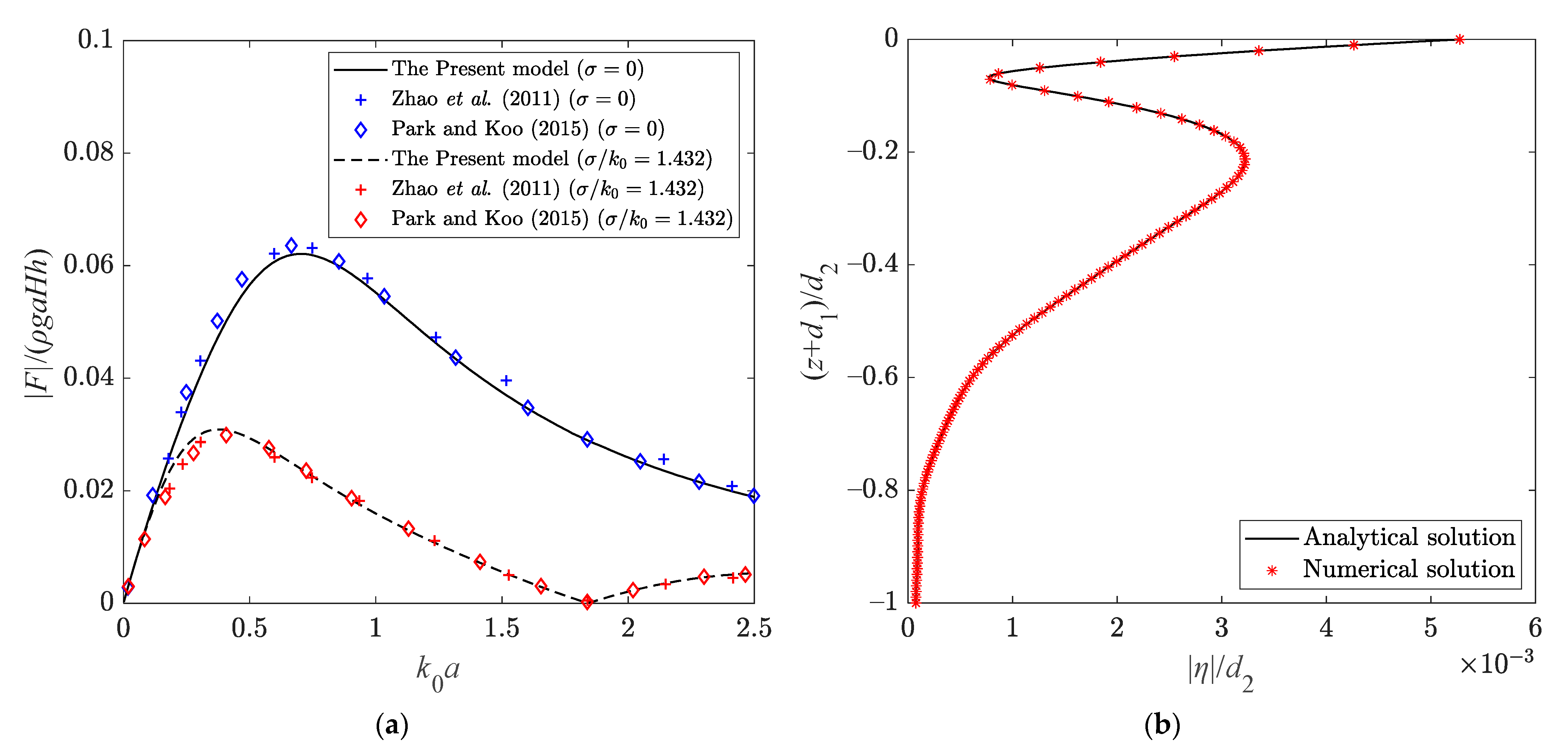
4. Convergence Studies and Model Validation

In Section 3, the derived solution is written in the form of the Fourier–Bessel series, and the infinite terms have been truncated after Nth and Mth terms. Theoretically, the calculated result is only valid when the solution converges with the increasing number of the series term. Therefore, convergence studies are required to determine the truncated terms to use for accurate results. For the convergence studies, the following parameters are adopted: H = 7 m, h = 200 m, a = 50 m, d1 = 0, d2 = 50 m, and G = 0.7. The nondimensional mooring spring constant α = ks/(msg) is 20, the nondimensional axial tensile force in the net γ = Q/(msgd2) is taken as 1, and the nondimensional net mass per unit length β = ms/(ρd22) = 0.001. The wave frequency ω varies from 0.2 rad/s to 1.4 rad/s at an interval of 0.4 rad/s. In Equation (18a–c), due to the orthogonality of cos(), the convergence of η is only determined by the series term generated by the wavenumbers from the dispersion relation Equation (14), so a control error ∆Er (N) versus the truncated term N is defined as
Δ E r ( N ) = | η ( d 1 d 2 2 ) , N + 1 η ( d 1 d 2 2 ) , N | | η ( d 1 d 2 2 ) , N | .
The variations of ∆Er (N) versus N from 1 to 50 are shown in Figure 3a. The results exhibit different convergency speeds for different wave frequencies, and the values of ∆Er (N) converge more slowly when the wave frequency is larger. Notably, when N > 30, the maximum control error is less than 2.25% for all cases. Alternatively, for the solution of the local wave field near the cage, the control error ∆Er (M) versus the truncated term M is defined as follows:
Δ E r ( M ) = | z = ( d 1 + d 2 ) d 1 θ = 0 2 π Δ φ ( a , θ , z ) , M + 1 z = ( d 1 + d 2 ) d 1 θ = 0 2 π Δ φ ( a , θ , z ) , M | | z = ( d 1 + d 2 ) d 1 θ = 0 2 π Δ φ ( a , θ , z ) , M | .
The curves of ∆Er (M) versus M from 1 to 50 are presented in Figure 3b. Similarly, if the wave frequency is lower, the control error will show a more rapid decay, and the control errors of the whole cases are closed to 0 for when M > 18. Based on the convergence studies, it is sufficient to take N = 30 and M = 20 to guarantee the accuracy for the solution of the imposed wave action and cage displacement.
In order to examine the correctness of the aforementioned formulations, consider a rigid impermeable or porous circular cage illustrated in [29,30] with the parameters of h = 5 m, a = 0.15 m, d1 = 0, and d2 = 0.3 m. The structural parameters adopted α = 1000, γ = 1000, and β = 1000 to ensure the cage motion is negligible. The nondimensional horizontal wave force acting on the cage versus the normalized wavenumber k0a is shown in Figure 4a. There are no significant differences between the present model and the aforementioned studies. A small discrepancy observed is because a horizontal impermeable plate is considered at the bottom of the cage in [29,30]. In addition, the current analytical solution of the cage deflection amplitude |η| is validated with the numerical solution generated by the Runge–Kutta method, where the parameters adopt the one in the convergence studies and ω = 1 rad/s. Figure 4b indicates that the derived analytical solution is completely consistent with the numerical results.

5. Hydroelastic Analysis of Fish Net Cage

This section discusses the hydroelastic spatial characteristics of the net cages by some numerical results. Five case groups were designed with various wave periods T (Cases A), net opening ratios G (Cases B), nondimensional mooring spring constants α (Cases C), nondimensional axial tensile forces γ in the net (Cases D), and immersed depths d1 of the cage (Cases E). The detailed parameter settings are shown in Table 1. In this analysis, a full-scale cage deployed in the marine aquaculture industry is considered, in which the cage radius a = 50 m, the cage height d2 = 50 m, and the dimensionless net mass per unit length β = 0.001. Moreover, the wave height H = 7 m and the water depth h = 200 m are adopted.

5.1. Hydrodynamic Behaviours

The present model can evaluate the distribution of the velocity potential Φ of the fluid domain and then derive its corresponding dynamic pressure and free surface elevations at a series of discretised points. Here, Cartesian coordinates (x = rcosθ and y = rsinθ) are established to facilitate the description of the results, where the central axis of the cage is located at the z-axis, and the incident wave propagates along the positive direction of the x-axis.
The free surface elevations ξ (m) around the cage with varied net opening ratios (Cases B1 to B4) are illustrated in Figure 5, in which ξ is calculated from Equation (30) in a domain of x = ± 200 m and y = ± 200 m. In this example, ξ adopted the values at time t = nT, n = 0, 1, 2, …, ∞, and the black circle is the demarcation between Regions 1 and 2. It can be observed that the presence of the cage causes perturbations to the wave surface, especially for the cage with an impermeable interface (i.e., net opening ratio G = 0). The transmitted wave passing through the cage will be attenuated, and its amplitude will gradually restore to its original state. This occurs because, when the scattered wave radiates away from the cage, the scattering potential gradually decays. Alternatively, the wave surface in the inner region of the cage also has different extents of attenuation, and the energy dissipation is the most severe, especially when G = 0. It is worth noting that, due to the blocking effect of the porous net, the water surface elevation inside the cage is affected by a certain lag in propagation when compared with the waves outside the cage. Furthermore, when the opening ratio of the net is gradually increased, the disturbance of the cylindrical net to the wave surface will gradually become weak, and the observed wave scattering becomes relatively minor for the cases with G > 0.3. In engineering practice, the adopted opening ratio of the fish net is usually greater than 0.6, so the influence of the net cage on the wave surface has become weak at this time.
Figure 6 shows the amplitude distributions of the pressure differences |∆p| on the windward and leeward sides of the net chamber in the incident wave direction. |∆p| is defined in Equation (27), and the results in Cases A1 to A4 with different wave periods are discussed. The maximum values of |∆p| are mainly concentrated at the top of the cylindrical cage, in which the maximum values are greater when the wave periods are smaller, that is 1.20 kPa (T = 4 s), 1.13 kPa (T = 6 s), 1.04 kPa (T = 8 s), and 0.89 kPa (T = 10 s). Nevertheless, the values of |∆p| at the lower part of the cage are relatively minor, and the values at its bottom end are close to 0. These results demonstrate that the wave has a more significant impact on the top part of the cage. Notably, more areas on the cage surface will withstand the pressure drop with high amplitudes under the wave action with longer periods, because short waves mainly concentrate on the free-water surface. Moreover, due to the energy dissipation of the transmitted wave, the pressure drop |∆p| on the leeward side is also slightly higher.

5.2. Structural Dynamic Responses
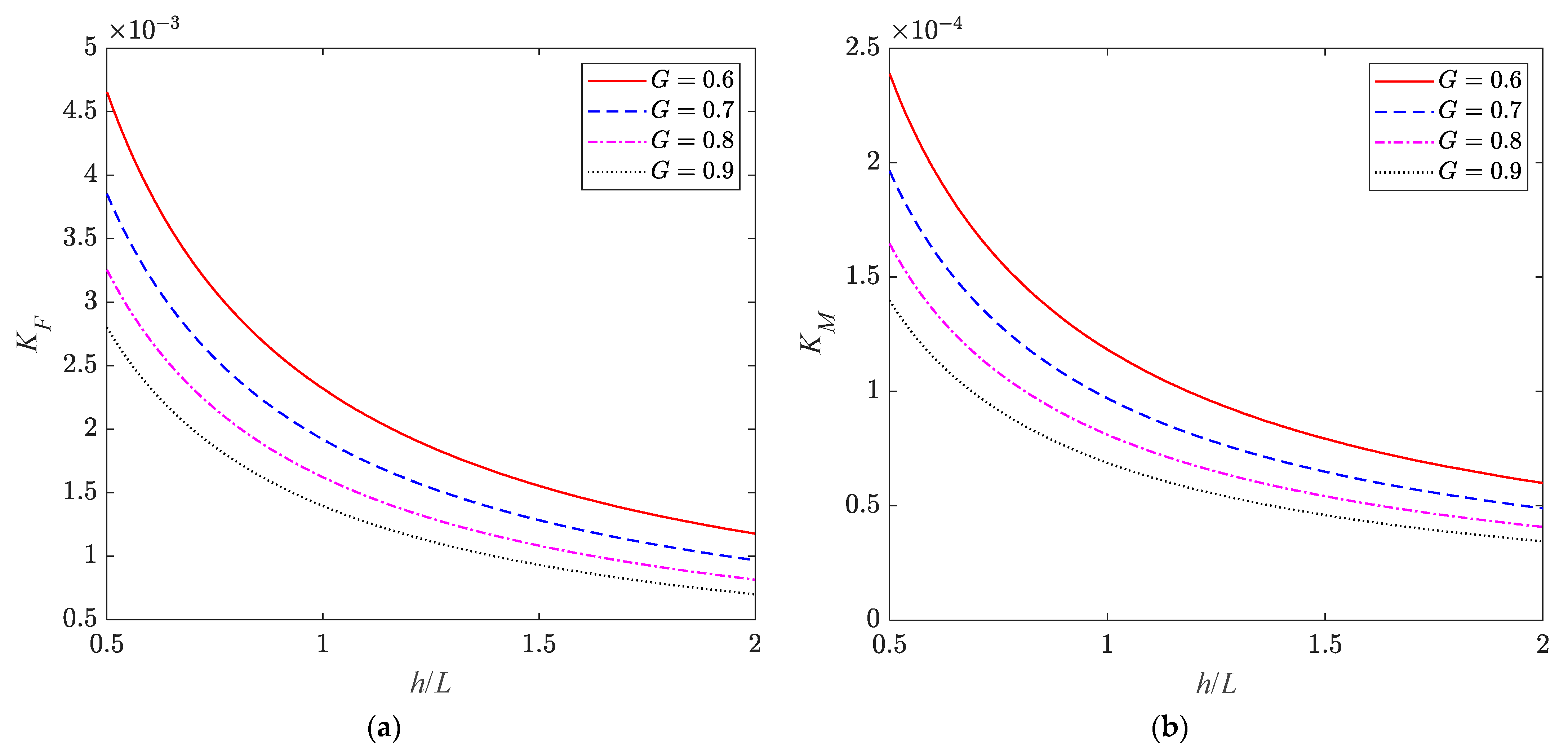
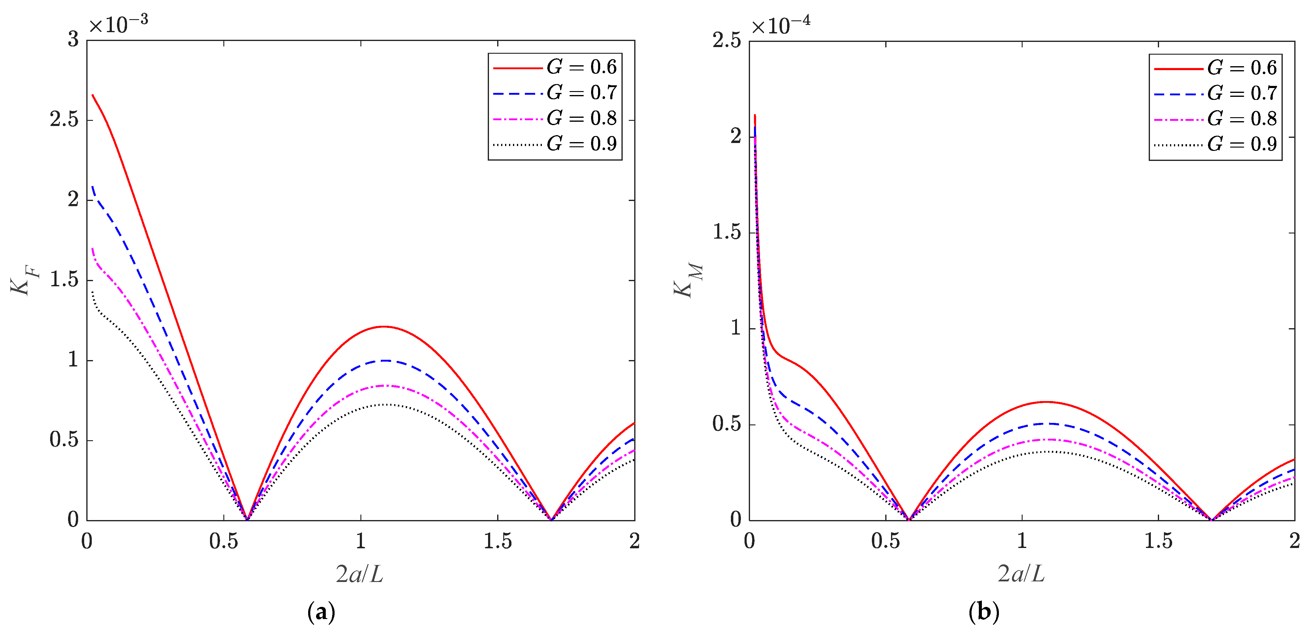
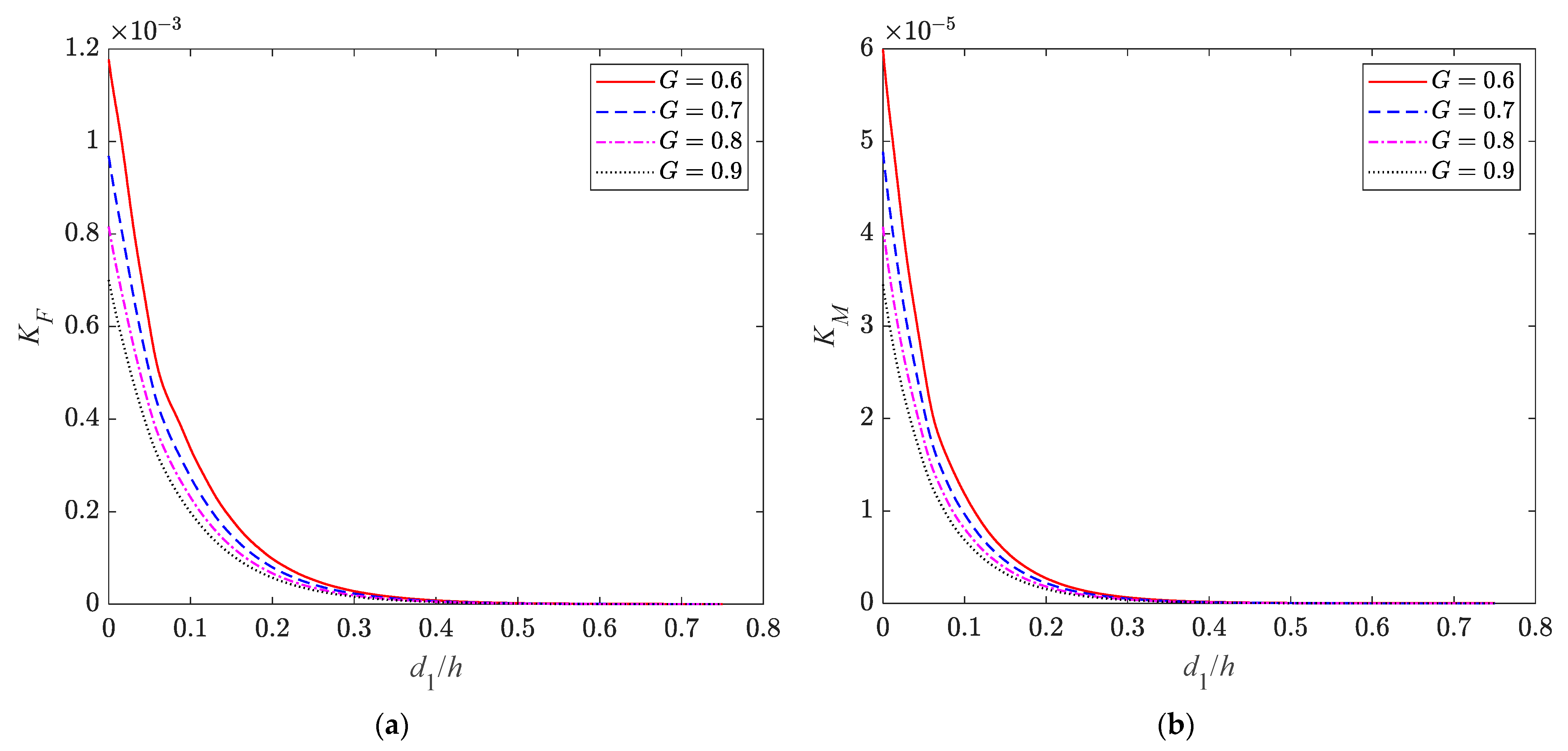
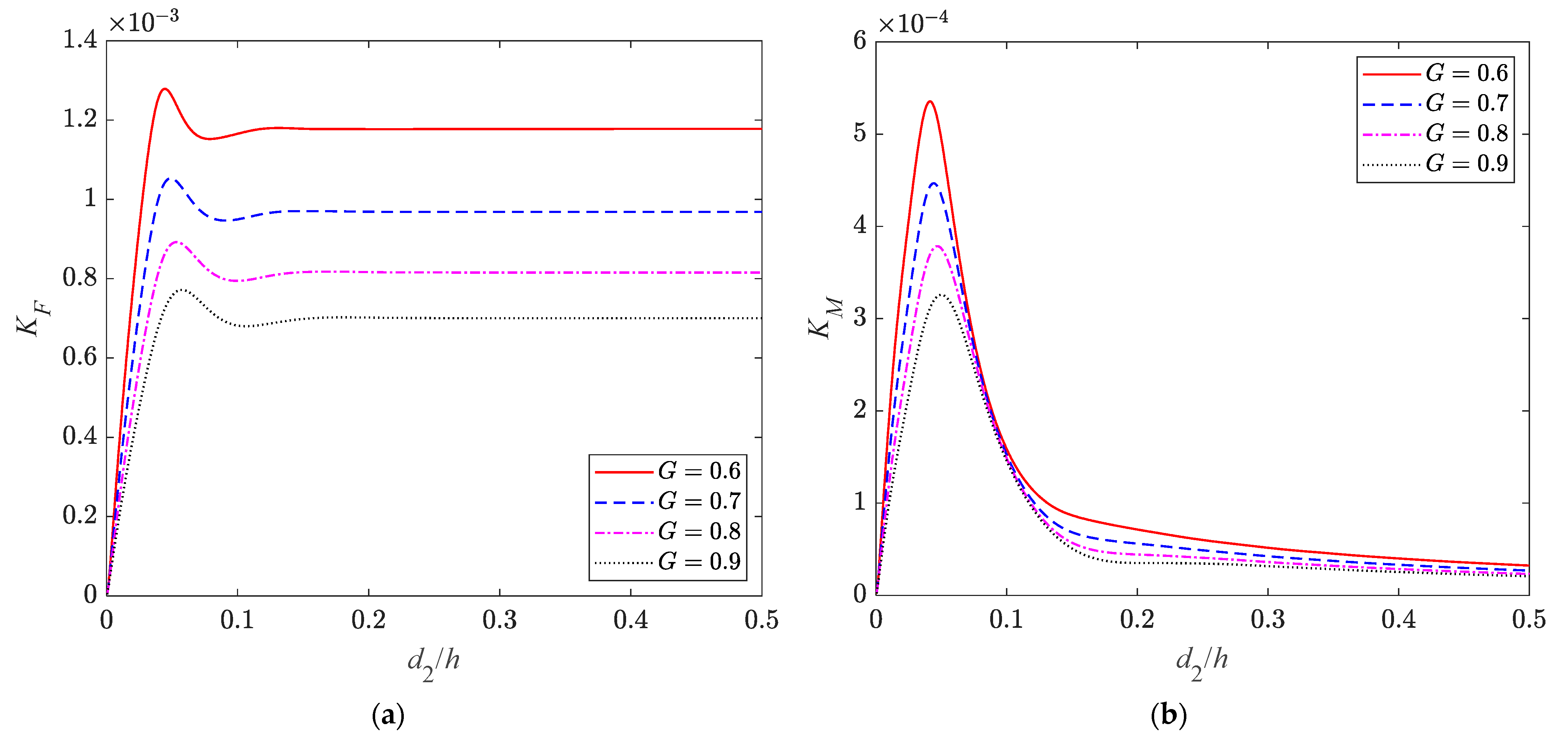
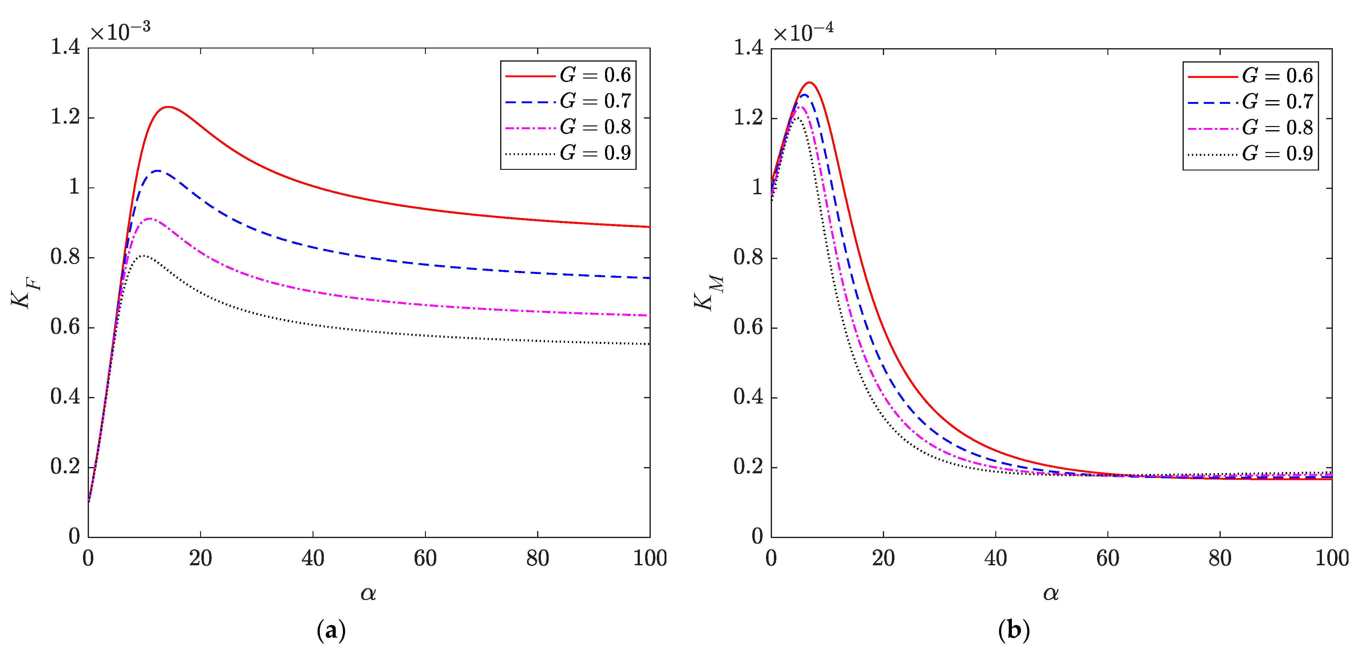
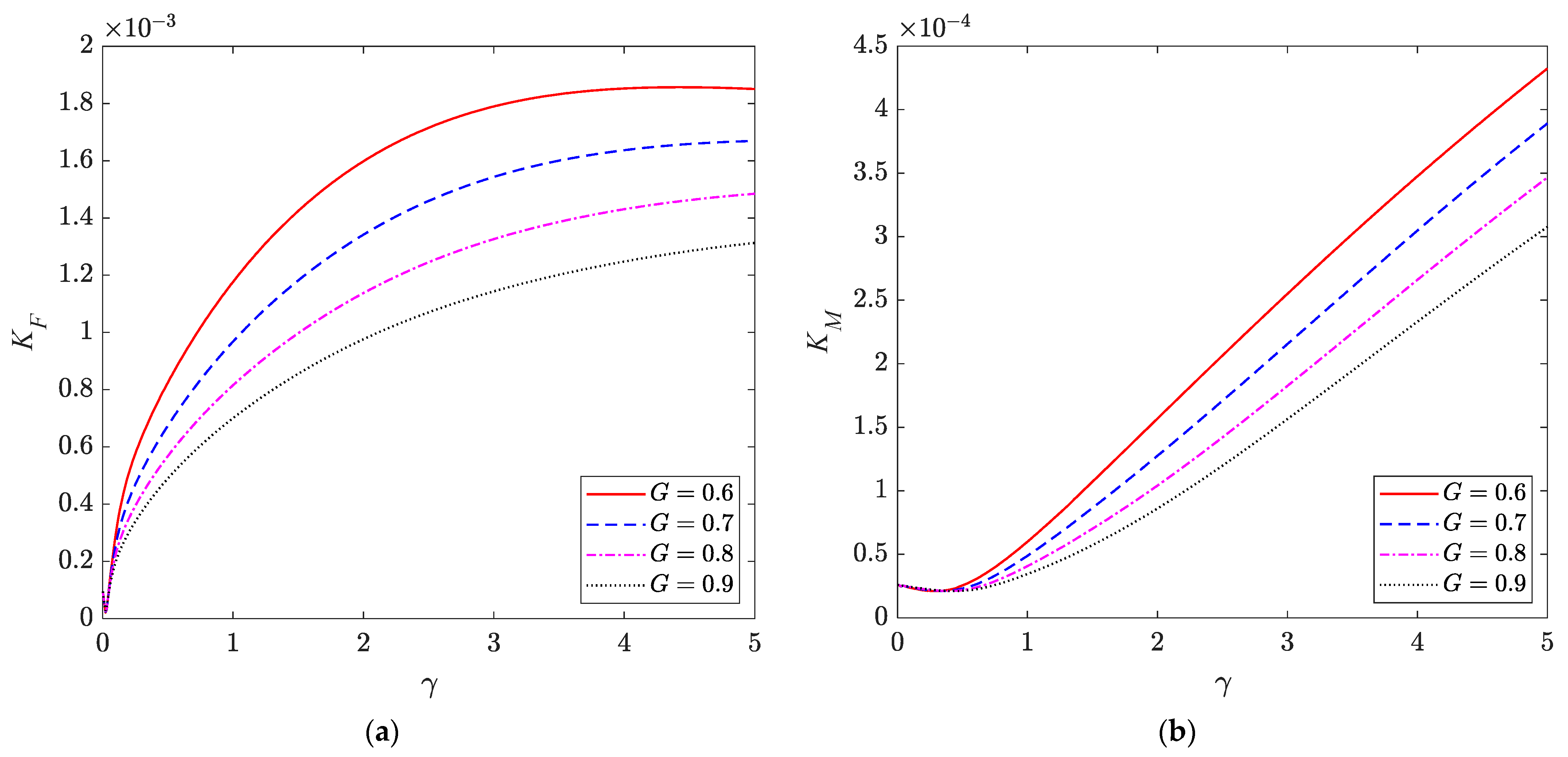
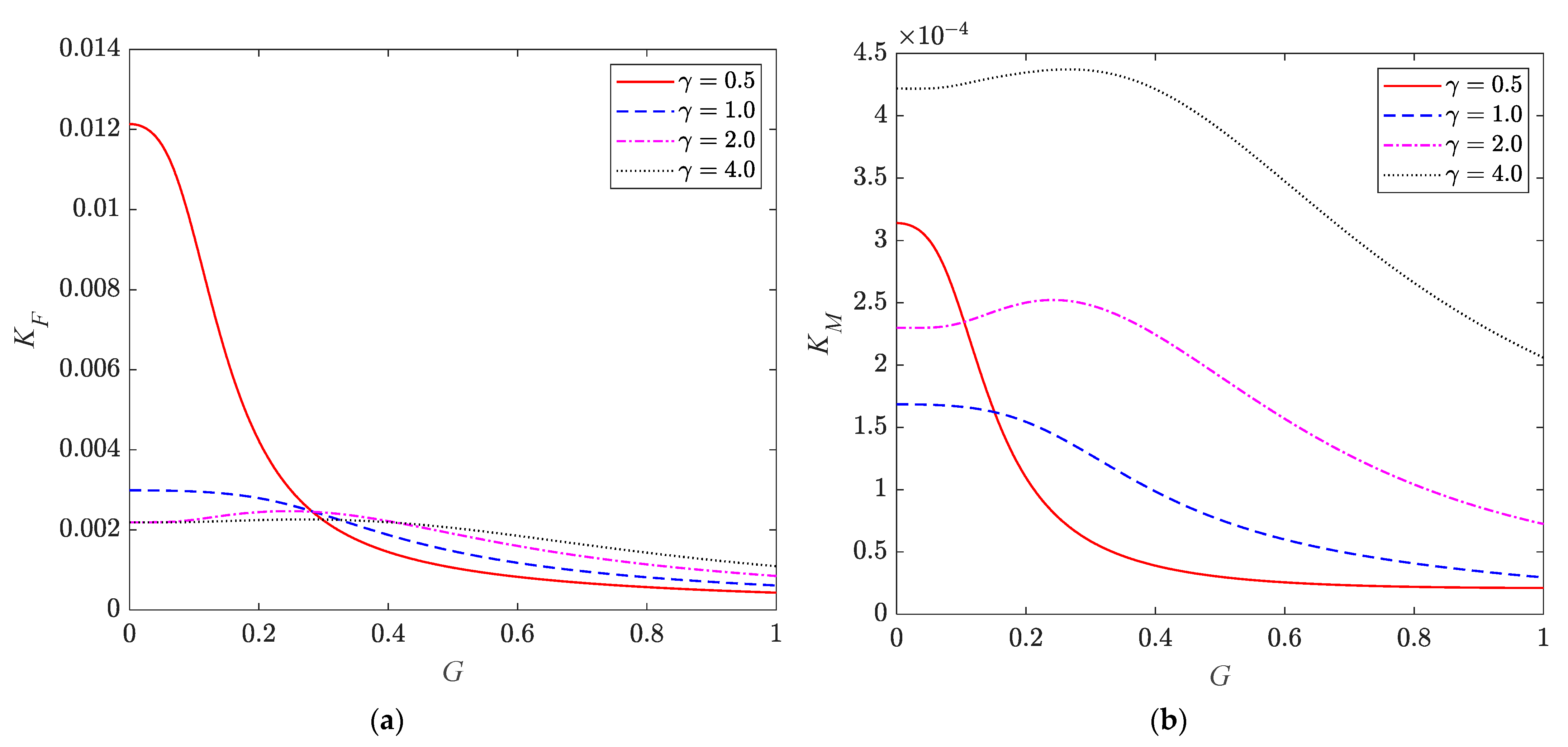
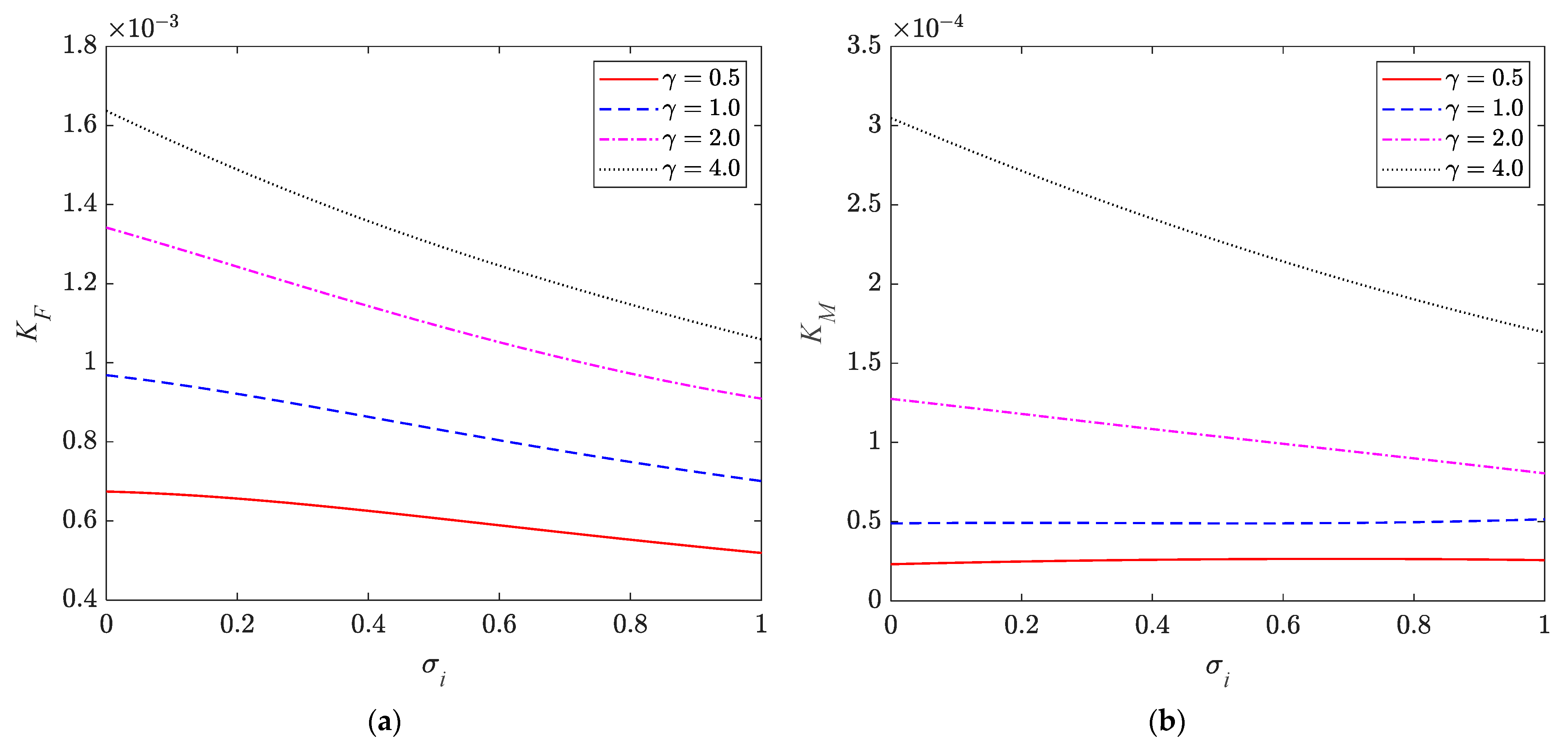
In this section, the structural dynamic responses of the net cage are investigated. Two important indices are presented: the nondimensional amplitude of the structural transverse deflection |η|/d2, and the nondimensional amplitude of the horizontal wave load per unit length Kf along the cage height. Following in the work of Mandal and Sahoo [21], Kf is defined as
K f = | f ( z ) | ρ g a H ,
in which the horizontal wave load per unit length f (z) is found from Equation (28). The curves of |η|/d2 and Kf versus the relative position defined as (z + d1)/d2 are plotted in Figure 7, Figure 8, Figure 9, Figure 10 and Figure 11.
It can be observed that the greater transverse deflection of the cylindrical net chamber occurs at the upper part of the cage height, and the horizontal wave load per unit length is the largest at the top end of the cage. At the bottom end of the structure, the values of |η|/d2 and Kf are the smallest. In addition, due to the assumption of structural edge constraints, the cage has a displacement at the top end (mooring constrained end), and the first derivatives to z are 0 at the bottom end (free end) for the curves of |η|/d2.
Figure 7 presents the results of Cases A1 to A4 with T varying from 4 s to 6 s with an interval of 2 s. It can be seen that when T = 8 s, the transverse deflection and wave load on the structure are much greater than the values of the other periods. That indicates that the net cage structure has a critical dynamic response at specific wave frequencies.
In Figure 8, Cases B5 to B8, when the porosity of the fish net increases, the transverse deflection amplitude at the upper part of the net chamber decreases but the value of the lower part slightly increases. With regard to the coefficient Kf, the values at the upper part of the cage have a greater difference, but when (z + d1)/d2 is smaller than −0.3, these differences are relatively small. This is because these cases are set as floating conditions, and the porous effect of the fish net will have a more significant blocking impact on the flow close to the wave surface.
In Figure 9, Cases C1 to C4 show the effect of the mooring cable stiffness, and there is also a fixed end case (η = 0 at z = −d1) presented. When α = 0.5, a weak spring stiffness results in the vanishing of peaks on the curves of |η|/d2 and a significant reduction of the normalized wave load Kf. Nevertheless, when α > 10, its influence on wave action becomes relatively minor.
Referring to Figure 10 (Cases D1 to D4), the distribution characteristics of |η|/d2 and Kf are similar when γ < 4. If the axial tension in the cage increases, the overall deformation of the cage can be suppressed, but the top displacement will increase. When γ = 4, there are no peaks along the curves of |η|/d2. Moreover, the wave action is enhanced to a certain extent for a stiffer net cage.
In Figure 11 (Cases D1 to D4), it can be seen that the wave effect will gradually become minimal as the diving depth of the cage increases. The corresponding structural deformation and wave load are also reduced significantly. This justifies the submergence of the cage into a deeper water level to avoid the strong surface waves. Moreover, the 3D shapes of the net chamber with the maximum deformation are plotted at different submerged depths in Figure 12, where the deflection values are magnified by an exaggerated scale of 5 times. Little wave response of the cage is observed when it is submerged at d1/h = 0.25.

6. Parametric Study

In order to investigate the effects of hydrodynamic and structural parameters on the wave loads, parametric studies are conducted in this section. The nondimensional amplitude of the hydrodynamic force KF in the horizontal direction and the nondimensional amplitude of the overturning moment KM with respect to the cage top are defined similarly to Mandal and Sahoo [21]:
K F = | F | ρ g a H h   and   K M = | M o | ρ g a H h ( d 1 + d 2 ) ,
in which the wave force F and the resulting overturning moment Mo are found from Equation (29). In the parametric studies, the following nondimensional hydrodynamic parameters are defined: the wave-effect parameter Cw = g/(ω2h) defined by Chwang [11], the incident wave steepness H/L, and the relative water depth h/L, where L is the incident wavelength. The parameters related to the cage dimensions include the relative diameter of the cage 2a/L, the relative dividing depths of the cage d1/h, and the relative height of the cage d2/h. Furthermore, the structural parameters have the nondimensional mooring spring constant α, the nondimensional axial tensile force in the net γ, the nondimensional net mass per unit length β, and the net opening ratio G.

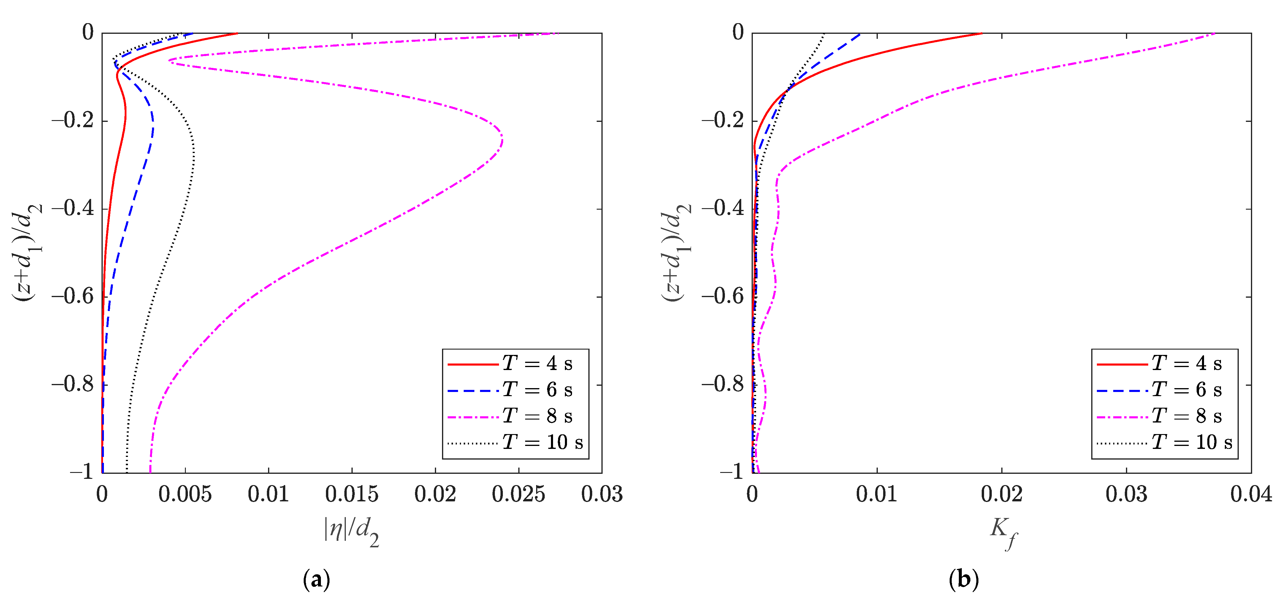
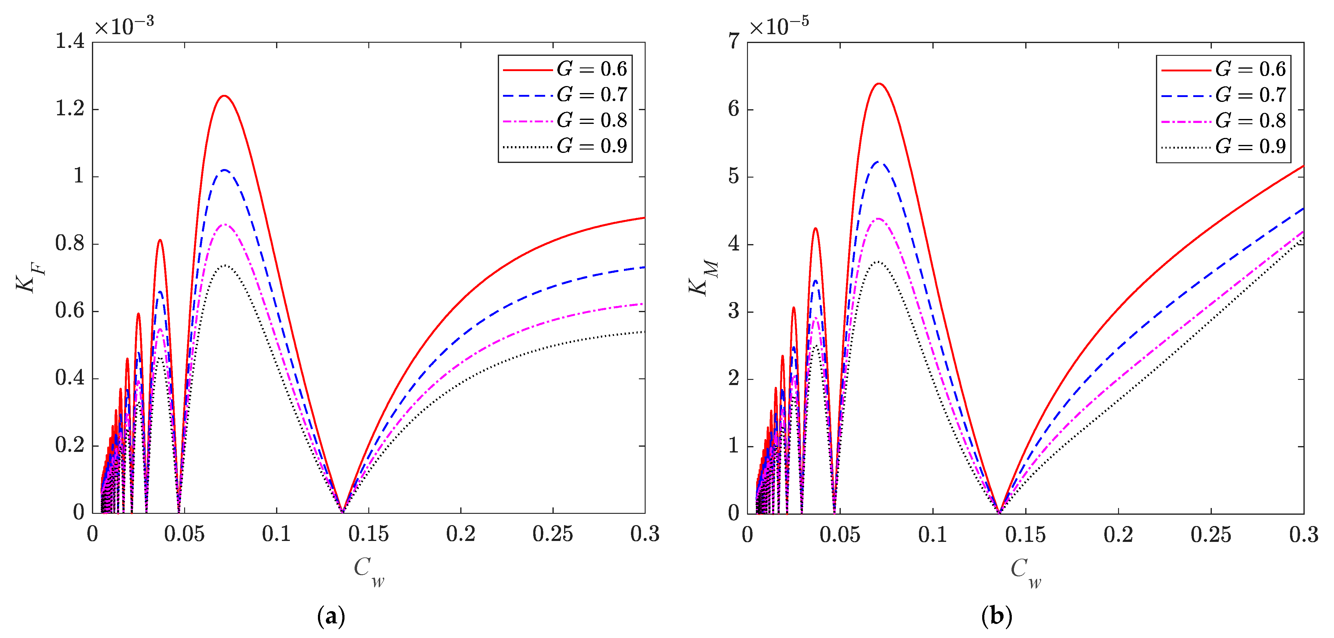
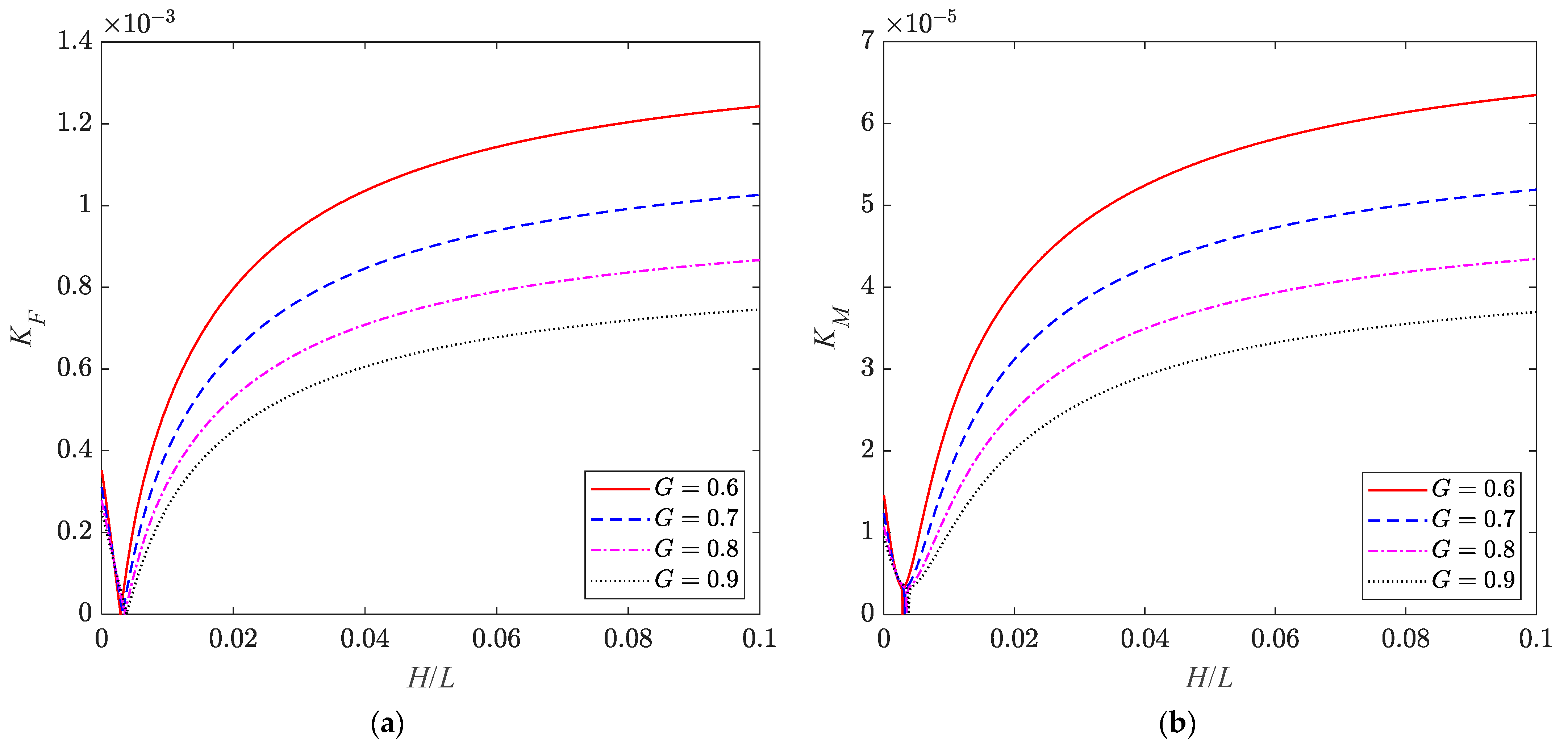
6.1. Hydrodynamic Conditions

The relationship between the wave load on the cage and the wave frequency is given in Figure 13. The curves of KF and KM versus Cw show multiple peak points and zero points. This may be because when the wavelength is at a specific value, the phase difference between the scattered waves in the outer region and the inner region near the circular cage is 180 degrees, resulting in wave attenuation. Conversely, if the phase difference is small, the wave action will be strengthened at this frequency.
As shown in Figure 14, the coefficients KF and KM are firstly decreased to the minimum values with the relative wave height H/L, and then they start to increase. In the small-amplitude wave theory, the velocity of the water particle has a linear relationship with the wave height. However, Equation (8b) indicates that the real part σr of the porous-effect parameter σ is changed related to the varied incident wave slope ε = Hk0/2. As a result, the wave load acting on the fish net does not increase linearly with the wave height.
Referring to Figure 15, when the water depth h increases from the values of the cage height to twice the wavelength, the values of KF and KM will decrease in opposition to the increase in the relative water depth h/L. It is worth noting that the water depth h is the denominator in the definition of the coefficients KF and KM, which may also contribute to the decrease in the values.

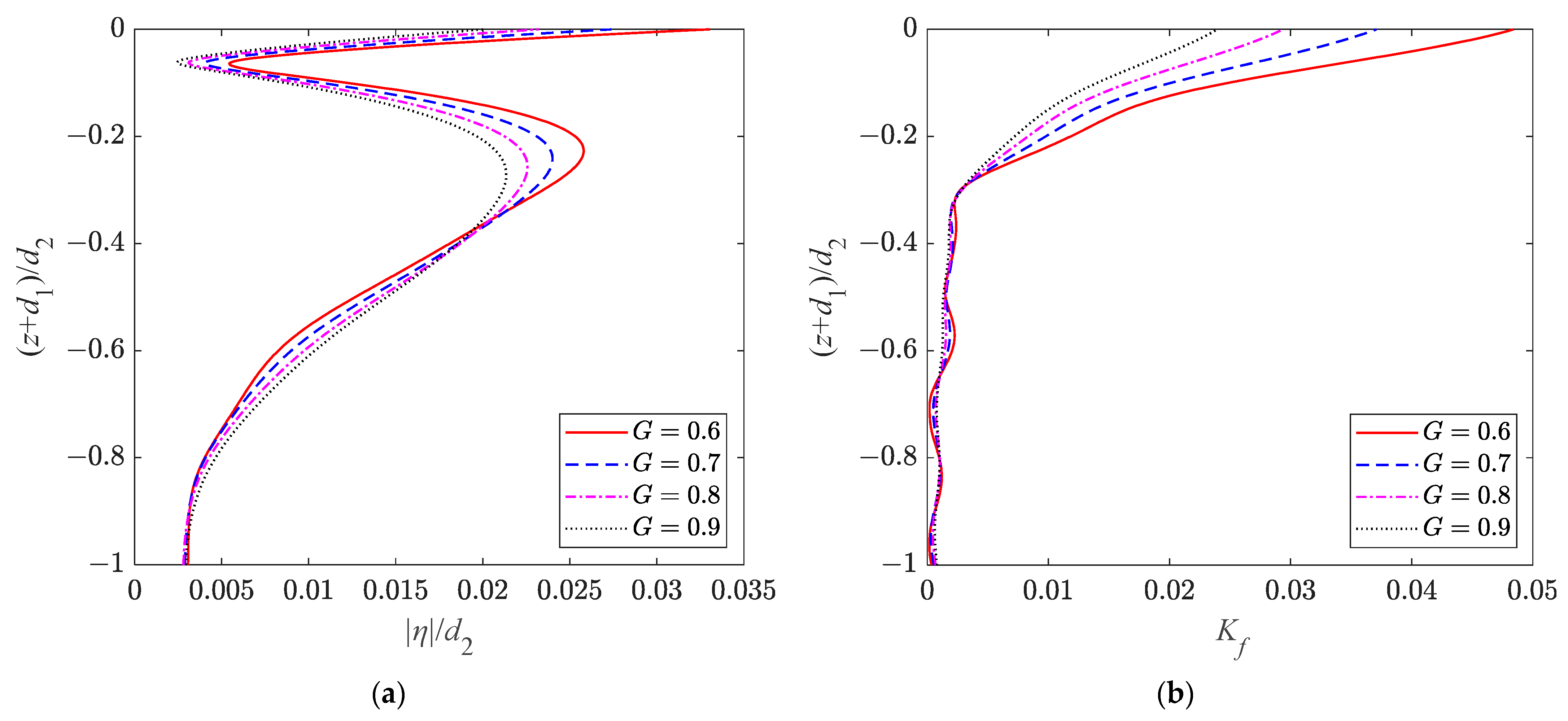
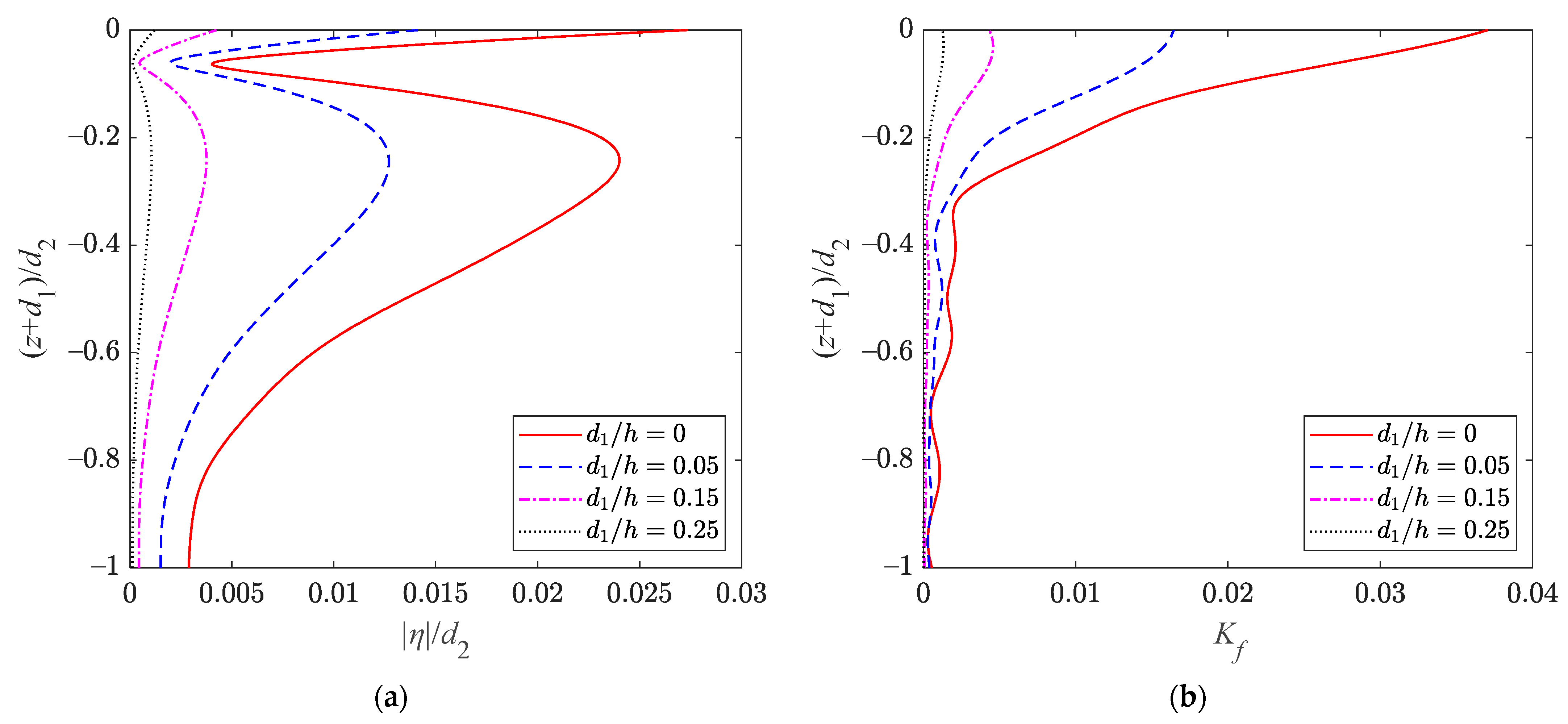
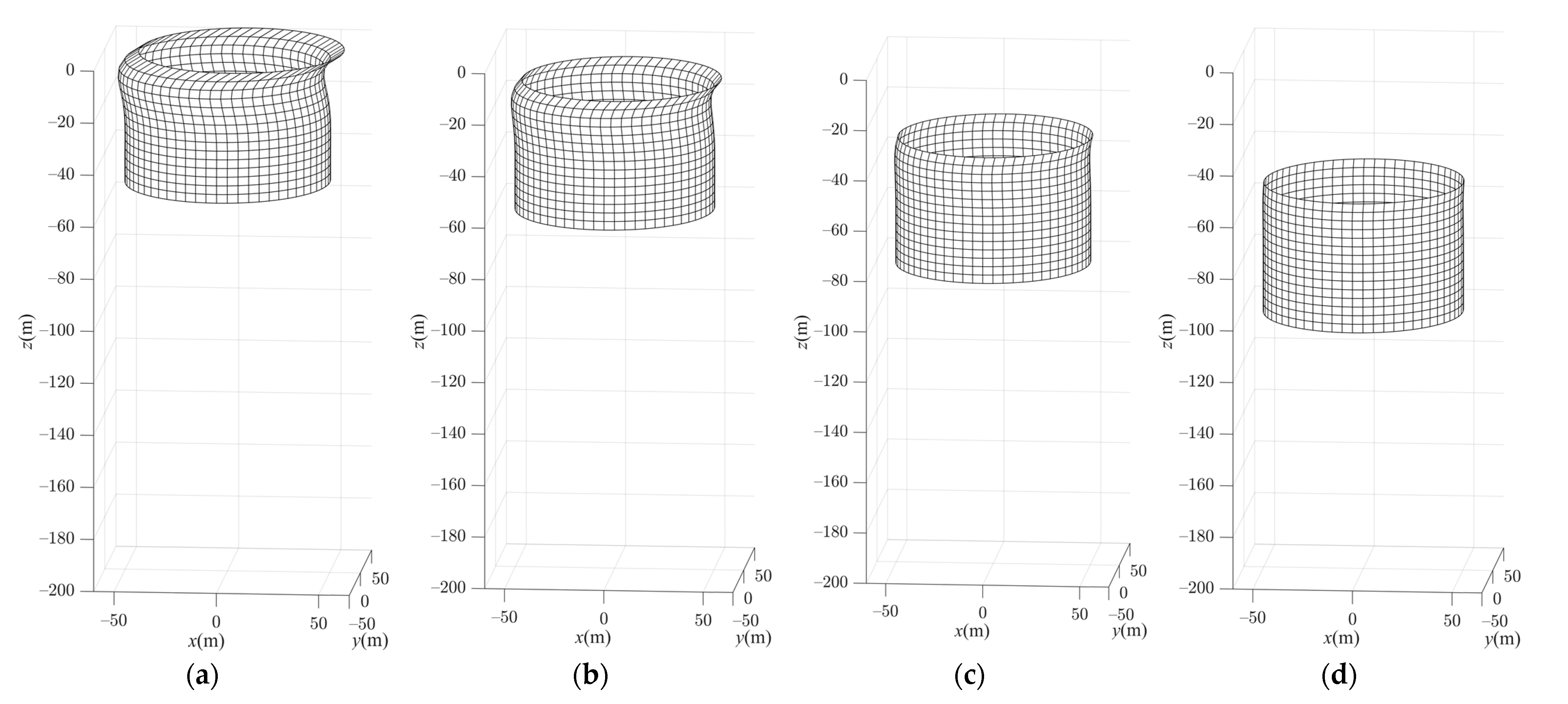
6.2. Cage Dimensions

As illustrated in Figure 16, at a constant wavelength, by increasing the diameter of the cage, the curves of the coefficients KF and KM will experience multiple peak points and zeros points as well, where the hydrodynamic force will vanish when 2a/L is around 0.59 and 1.70. The wave force on the cylindrical cage has a similar variation under various wave frequencies. Therefore, the ratio of the diameter of the circular cage to the wavelength is crucial in engineering design.
If the cage is submerged to a deeper location underwater, the effect of surface waves will be weakened, so the coefficients KF and KM will be reduced in Figure 17. However, this decreasing trend will slow down as the wave action has been minimal at extremely deep water levels.
The effect of cage height on the wave load is shown in Figure 18. Attentively, as the cage height d2 increases, the axial tensile force Q and the mass per unit length ms of the net chamber will increase if the defined nondimensional parameters γ and β remain constant. This is unreasonable. Therefore, the relevant structural parameters are assumed to take the following values: Q/(msga) = 1 and ms/(ρa2) = 0.001. Assuming that the top of the cage is at the mean water level, with the increase of the cage height, the values of KF and KM will rapidly rush to the peak point, and then begin to decrease. The magnitude of KF will remain constant after d2/h = 0.2. This is because the imposed wave pressure has been already negligible at the part of the cage close to the deep water level.

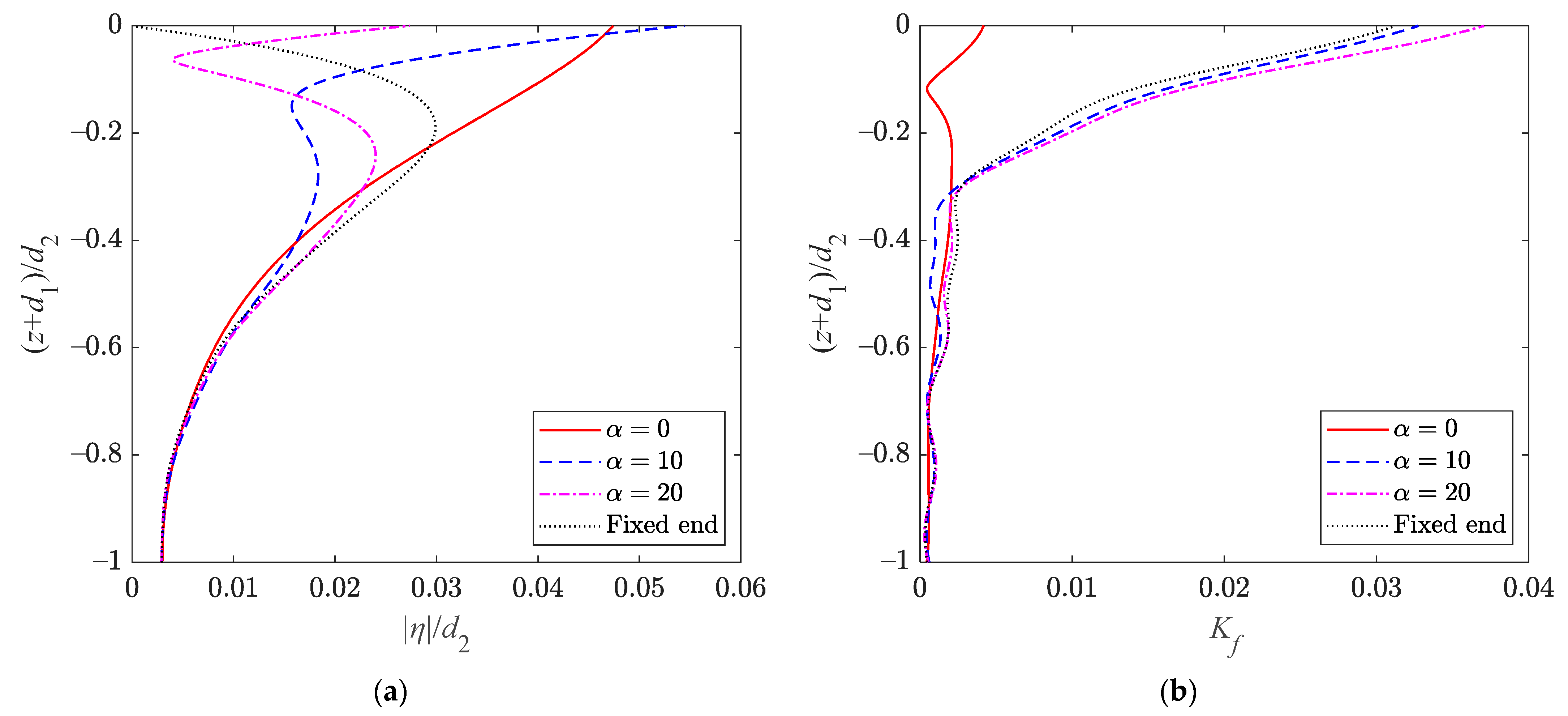
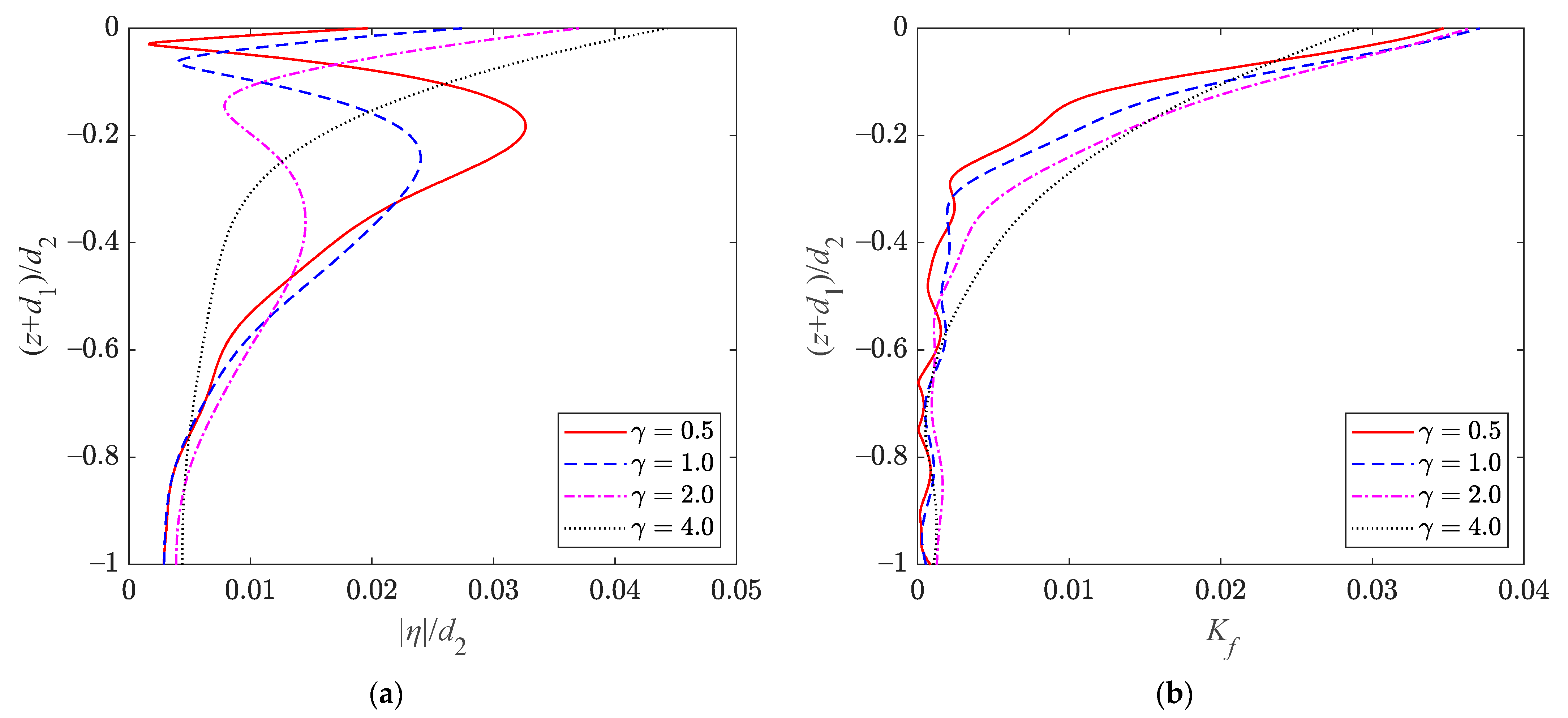
6.3. Structural Parameters

It can be observed from Figure 19 that as the spring stiffness of the mooring rope increases, the wave action coefficients KF and KM increase to reach a peak value, and then gradually decrease. When α > 40, this trend is also slowed down.
The curves in Figure 20 show that the coefficients KF and KM are greater with respect to increasing γ. This might be explained by the fact that more momentum of the fluid is dissipated when impacting on stiffer structures. However, the curves of KF present a slowdown in the growth trend, but KM increases approximately linearly when γ > 1.
The mass of the fish net is generally determined by different net materials or biomass effects. In Figure 21, in order to ensure a constant mooring stiffness and axial tension in the net, we have taken that ks/(ρgd22) = 0.02 and Q/(ρgd23) = 0.001. It can be observed that, with increasing β from 0 to 0.01, the wave force coefficient KF initially decreases and then increases slowly, but the moment coefficient KM decreases slightly first and then increases rapidly.
In Figure 22, under different axial tensions in the net, the coefficients KF and KM show different varying trends when G < 0.4. However, the increase in the porosity of the fish net is conducive for reducing the wave action when the opening ratio is over 0.4. Consequently, it is important that the porosity of the net is kept high, and it is essential to clean the net often to remove the biofouling organisms and hydroids to reduce the wave load on the fish cage. Notably, when the net opening ratio G = 1, i.e., the net does not exist, the predicted wave forces are not zero. According to [25], theoretically, the porous effect parameter σ should go to infinity when the net interface becomes completely permeable, but Equation (8b) obviously does not obey this scenario. Therefore, a more suitable formula for the porous effect parameter is required in future studies.
On the other hand, although the assumption in Equation (8a,b) ignores the fluid inertia effect for the flow penetrating through the net interface, its influence still needs to be discussed. An empirical formula of σi provided by Ito et al. [25] indicates that most values are in a range of less than 1 for the cube net cage. Here, by assuming that the values of σi for most cylindrical net cages are less than 1, the variations of KF and KM with respect to σi from 0 to 1 are shown in Figure 23. These curves indicate a significant influence of σi when the values of γ are high. A minor effect of σi is seen when γ is smaller, especially for the coefficient KM. As a result, the porous effect of the fish net will exhibit different properties with different axial tensions, and thus the fluid inertia effect parameter σi still needs further investigation.

7. Conclusions

A semi-analytical model for wave–cage interaction is established based on the potential flow theory to investigate the hydroelastic behaviour of a cylindrical fish net cage under wave actions. The net cage is modelled as a flexible porous cylinder and its motions are governed by the string vibration equations. By separating variables, the general solution of this physics problem can be expressed by the Fourier–Bessel series. The unknown constants in these series are determined from matching the boundary conditions and the least squares method. Based on this study, the following conclusions may be drawn:
(1)
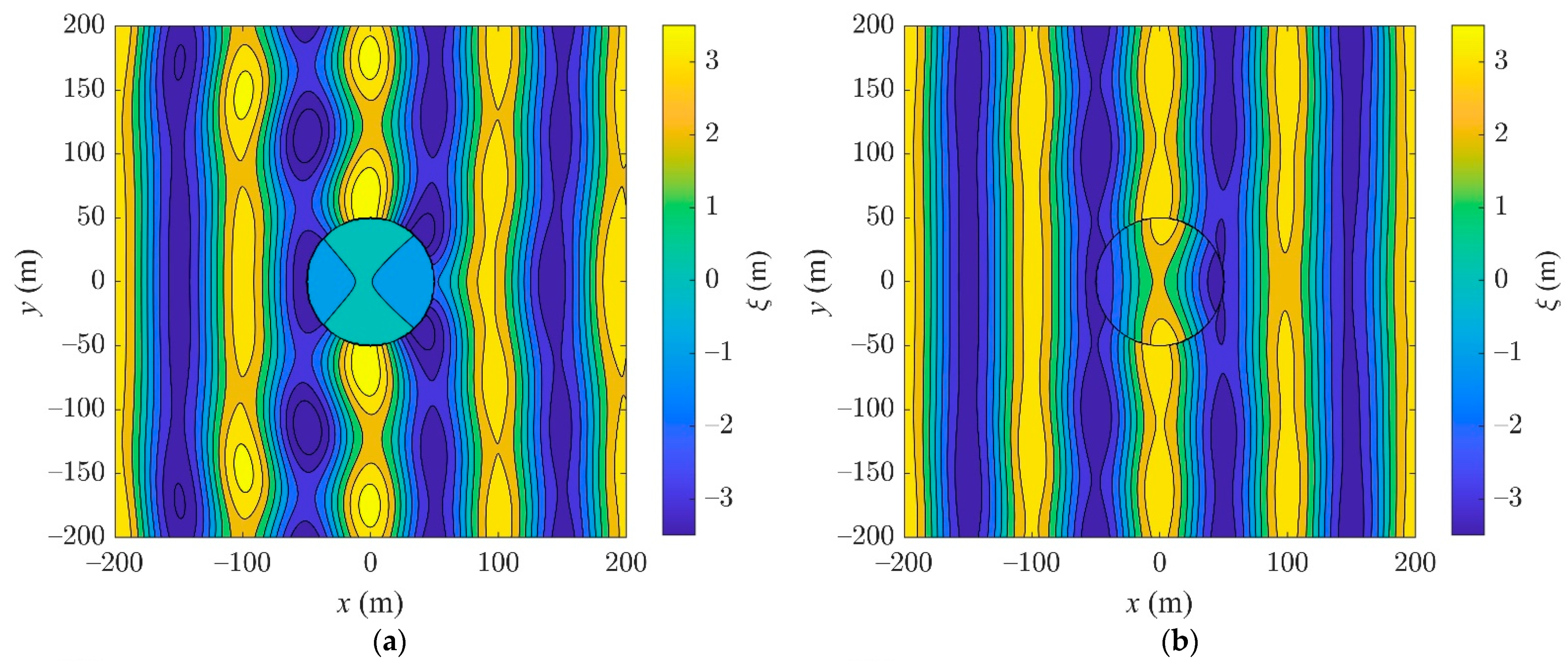
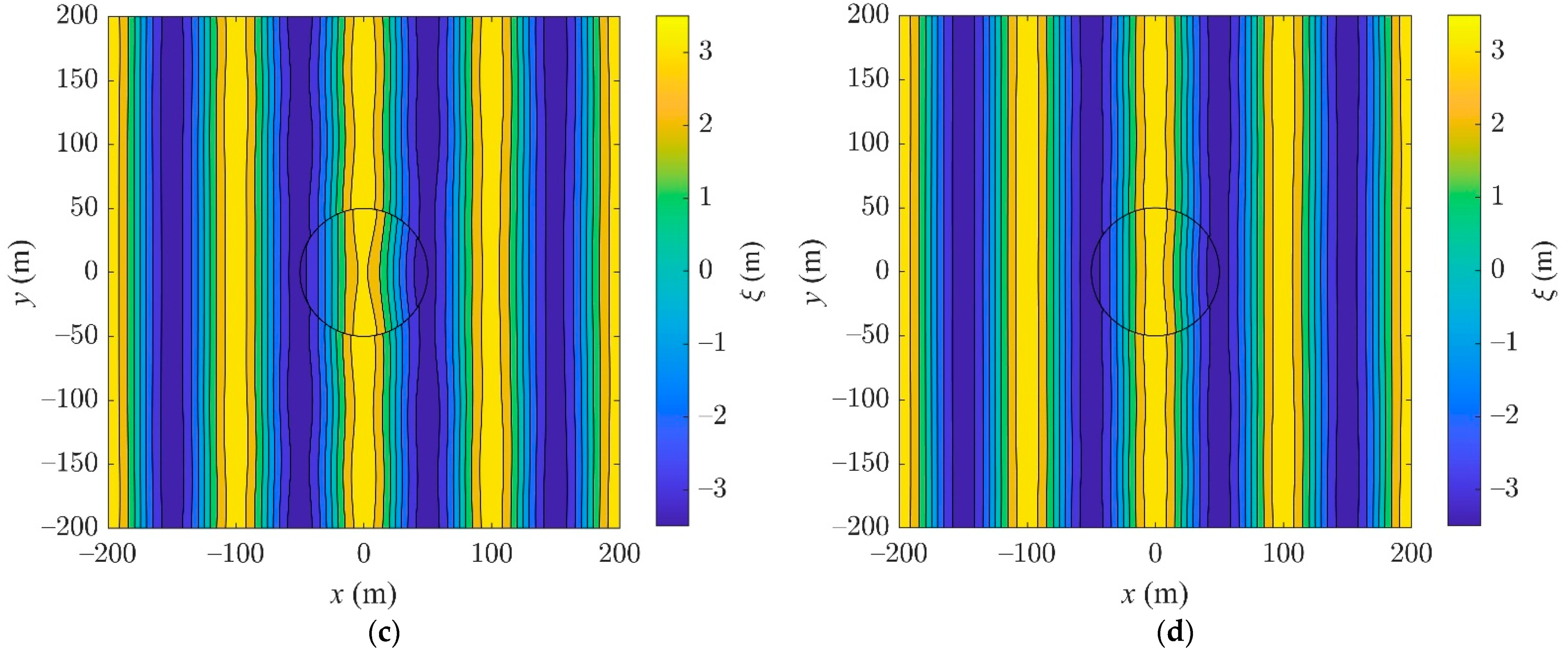
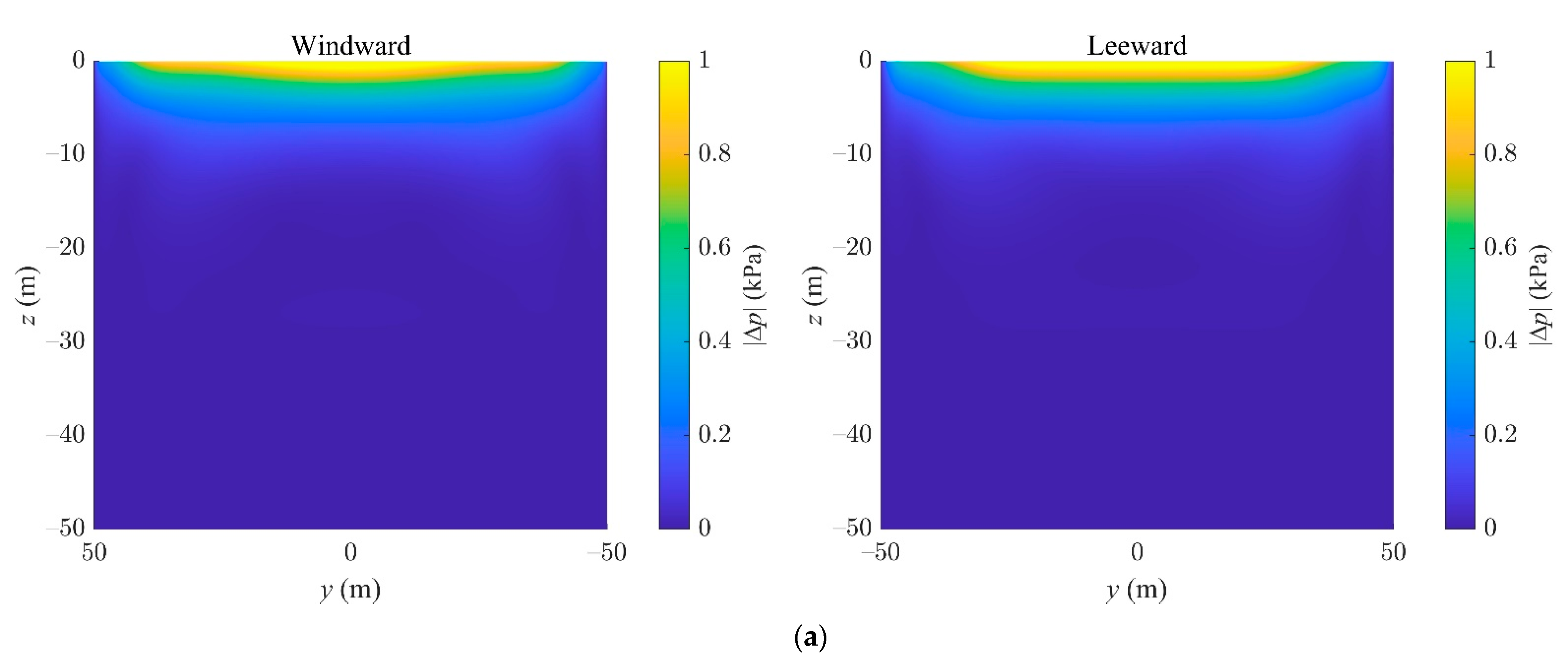
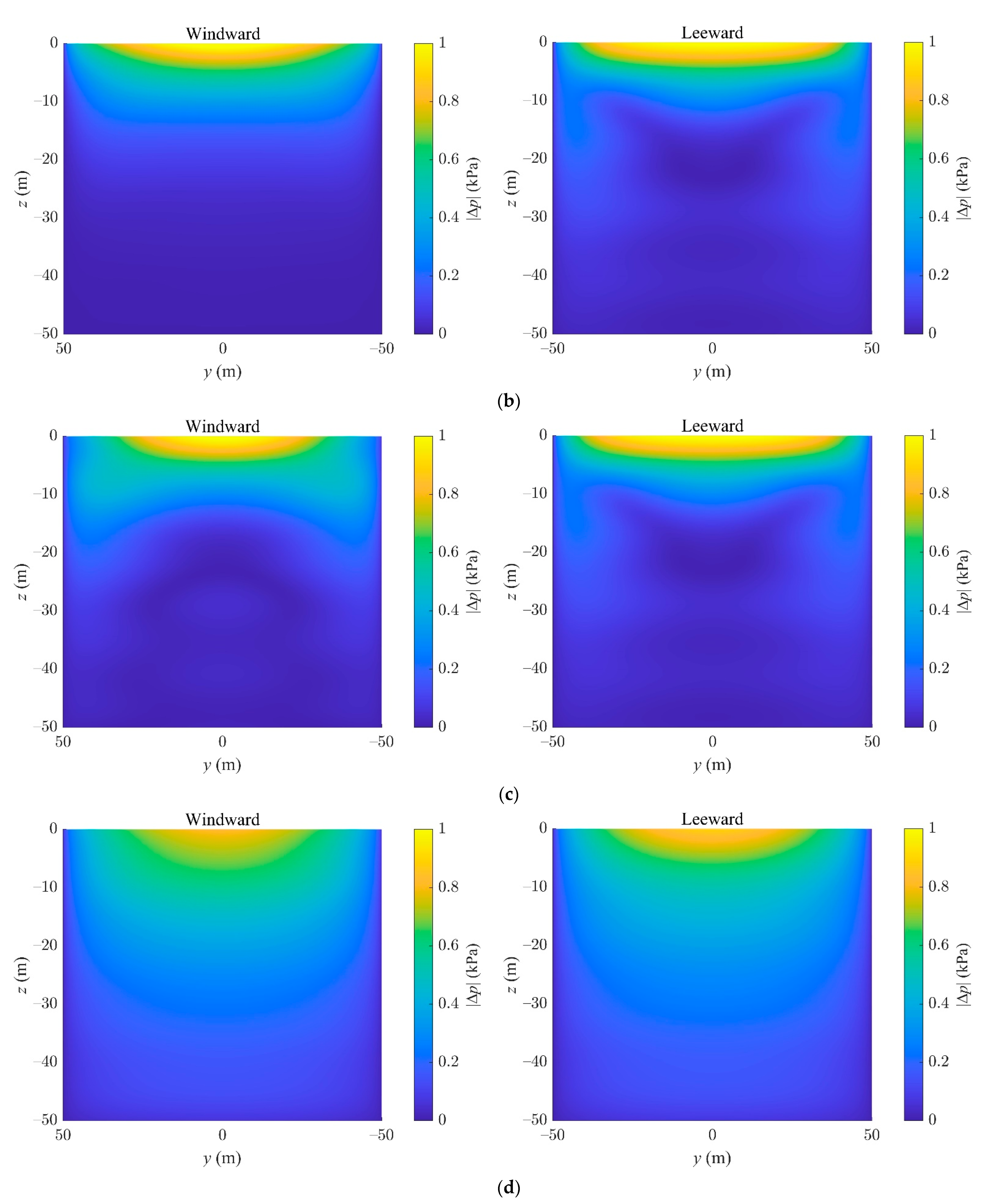
The disturbance caused by the cage to the wave surface is weaker when the opening ratio of the net is greater than 0.3. The wave actions are stronger near the mean water level, as expected. Consequently, a submersible cage is recommended to avoid the high surface-wave energy.
(2)
Under different mooring stiffness and axial tension in the net, the deflection amplitude of the cage presents different distribution characteristics.
(3)
The net chamber will be subjected to critical wave responses at particular frequencies, but some specific ratios of the cage diameter to the wavelength might cause the vanishing of the wave force and the overturning moment on the cage.
(4)
Appropriately increasing the porosity and reducing the axial tension of the net chamber are beneficial in reducing the wave load.
(5)
The porous effect of the fish net is significantly impacted by the axial tension in the cage.
The present study reveals some mechanical characteristics of the interaction between the wave and the net cage and provides a reference for the design and application of fish cage systems. However, the theories and formulas used in the present study are all based on linear models, so they cannot solve nonlinear problems in wider scenarios, such as nonlinear waves, quadratic porous flow models, etc., and the structural vibration equation may be oversimplified. Those problems will be considered and resolved in future studies.

Author Contributions

Conceptualization, M.M., H.Z., D.-S.J. and C.M.W.; methodology, M.M.; validation, M.M.; formal analysis, M.M.; writing—original draft preparation, M.M.; writing—review and editing, H.Z., D.-S.J. and C.M.W.; supervision, H.Z., D.-S.J. and C.M.W. All authors have read and agreed to the published version of the manuscript.

Funding

The postgraduate scholarship of Griffith University, Australia, the top-up scholarship of Blue Economy Cooperative Research Centre, Australia and HDR Journal Publishing and Editorial Assistance Scheme (JPEAS) of Griffith Cities Research Institute, Australia.

Data Availability Statement

The main data provided in the present study is generated by the numerical model developed from this paper. For the model validation in Figure 4a, the compared data is from [29] and [30].

Acknowledgments

The first author is very grateful to Griffith University and the Blue Economy CRC for providing scholarships to support this research. In addition, the first author would like to thank Griffith Cities Research Institute for providing HDR Journal Publishing and Editorial Assistance Scheme (JPEAS).

Conflicts of Interest

The authors declare that they have no direct or potential financial and personal relationship with other people or organizations which could inappropriately influence (bias) their work. The authors confirm that the manuscript has been read and approved by all designated authors, and that no one else meets the author criteria but is not listed. We further confirm that the order of authors listed in the manuscript has been approved by all of us.

References

  1. FAO. The State of World Fisheries and Aquaculture 2020; Food and Agriculture Organization of the United Nations: Rome, Italy, 2020. [Google Scholar]
  2. Zhou, X. Brief Overview of World Aquaculture Production: An Update with Latest Available 2017 Global Production Data. FAO Aquac. Newslett. 2019, 60, 6–8. [Google Scholar]
  3. Chen, D.; Wang, C.; Zhang, H. Examination of net volume reduction of gravity-type open-net fish cages under sea currents. Aquac. Eng. 2021, 92, 102128. [Google Scholar] [CrossRef]
  4. Tsukrov, I.; Eroshkin, O.; Fredriksson, D.; Swift, M.; Celikkol, B. Finite element modeling of net panels using a consistent net element. Ocean Eng. 2003, 30, 251–270. [Google Scholar] [CrossRef]
  5. Zhan, J.; Jia, X.; Li, Y.; Sun, M.; Guo, G.; Hu, Y. Analytical and experimental investigation of drag on nets of fish cages. Aquac. Eng. 2006, 35, 91–101. [Google Scholar] [CrossRef]
  6. Li, Y.-C.; Zhao, Y.-P.; Gui, F.-K.; Teng, B. Numerical simulation of the hydrodynamic behaviour of submerged plane nets in current. Ocean Eng. 2006, 33, 2352–2368. [Google Scholar] [CrossRef]
  7. Zhao, Y.-P.; Li, Y.-C.; Dong, G.; Gui, F.-K.; Wu, H. An experimental and numerical study of hydrodynamic characteristics of submerged flexible plane nets in waves. Aquac. Eng. 2008, 38, 16–25. [Google Scholar] [CrossRef]
  8. Kristiansen, T.; Faltinsen, O.M. Modelling of current loads on aquaculture net cages. J. Fluids Struct. 2012, 34, 218–235. [Google Scholar] [CrossRef]
  9. Bi, C.-W.; Zhao, Y.-P.; Dong, G.-H.; Xu, T.-J.; Gui, F.-K. Numerical simulation of the interaction between flow and flexible nets. J. Fluids Struct. 2014, 45, 180–201. [Google Scholar] [CrossRef]
  10. Martin, T.; Tsarau, A.; Bihs, H. A numerical framework for modelling the dynamics of open ocean aquaculture structures in viscous fluids. Appl. Ocean Res. 2021, 106, 102410. [Google Scholar] [CrossRef]
  11. Chwang, A.T. A porous-wavemaker theory. J. Fluid Mech. 1983, 132, 395–406. [Google Scholar] [CrossRef]
  12. Yu, X.; Chwang, A.T. Wave-Induced Oscillation in Harbor with Porous Breakwaters. J. Waterw. Port Coast. Ocean Eng. 1994, 120, 125–144. [Google Scholar] [CrossRef]
  13. Lee, M.M.; Chwang, A.T. Scattering and radiation of water waves by permeable barriers. Phys. Fluids 2000, 12, 54–65. [Google Scholar] [CrossRef] [Green Version]
  14. Sankarbabu, K.; Sannasiraj, S.; Sundar, V. Interaction of regular waves with a group of dual porous circular cylinders. Appl. Ocean Res. 2007, 29, 180–190. [Google Scholar] [CrossRef]
  15. Park, M.-S.; Koo, W.-C.; Choi, Y.-R. Hydrodynamic interaction with an array of porous circular cylinders. Int. J. Nav. Arch. Ocean Eng. 2010, 2, 146–154. [Google Scholar] [CrossRef] [Green Version]
  16. Abul-Azm, A.; Williams, A. Interference effects between flexible cylinders in waves. Ocean Eng. 1987, 14, 19–38. [Google Scholar] [CrossRef]
  17. Yip, T.; Sahoo, T.; Chwang, A.T. Trapping of surface waves by porous and flexible structures. Wave Motion 2002, 35, 41–54. [Google Scholar] [CrossRef]
  18. Behera, H.; Sahoo, T. Hydroelastic analysis of gravity wave interaction with submerged horizontal flexible porous plate. J. Fluids Struct. 2015, 54, 643–660. [Google Scholar] [CrossRef]
  19. Mandal, S.; Datta, N.; Sahoo, T. Hydroelastic analysis of surface wave interaction with concentric porous and flexible cylinder systems. J. Fluids Struct. 2013, 42, 437–455. [Google Scholar] [CrossRef]
  20. Su, W.; Zhan, J.-M.; Huang, H. Analysis of a porous and flexible cylinder in waves. China Ocean Eng. 2015, 29, 357–368. [Google Scholar] [CrossRef]
  21. Mandal, S.; Sahoo, T. Gravity wave interaction with a flexible circular cage system. Appl. Ocean Res. 2016, 58, 37–48. [Google Scholar] [CrossRef]
  22. Selvan, S.A.; Gayathri, R.; Behera, H.; Meylan, M.H. Surface wave scattering by multiple flexible fishing cage system. Phys. Fluids 2021, 33, 037119. [Google Scholar] [CrossRef]
  23. Guo, Y.; Mohapatra, S.; Soares, C.G. Review of developments in porous membranes and net-type structures for breakwaters and fish cages. Ocean Eng. 2020, 200, 107027. [Google Scholar] [CrossRef]
  24. Li, M.; Zhang, H.; Guan, H.; Lin, G. Three-dimensional investigation of wave–pile group interaction using the scaled boundary finite element method. Part I: Theoretical developments. Ocean Eng. 2013, 64, 174–184. [Google Scholar] [CrossRef] [Green Version]
  25. Ito, S.; Kinoshia, T.; Bao, W. Hydrodynamic behaviors of an elastic net structure. Ocean Eng. 2014, 92, 188–197. [Google Scholar] [CrossRef]
  26. Liu, H.-F.; Bi, C.-W.; Zhao, Y.-P. Experimental and numerical study of the hydrodynamic characteristics of a semisubmersible aquaculture facility in waves. Ocean Eng. 2020, 214, 107714. [Google Scholar] [CrossRef]
  27. Sommerfeld, A. Partial Differential Equations in Physics; Elsevier Science & Technology: Burlington, MA, USA, 1949. [Google Scholar] [CrossRef] [Green Version]
  28. Liu, Z.; Mohapatra, S.; Soares, C. Finite Element Analysis of the Effect of Currents on the Dynamics of a Moored Flexible Cylindrical Net Cage. J. Mar. Sci. Eng. 2021, 9, 159. [Google Scholar] [CrossRef]
  29. Zhao, F.; Bao, W.; Kinoshita, T.; Itakura, H. Theoretical and Experimental Study on a Porous Cylinder Floating in Waves. J. Offshore Mech. Arct. Eng. 2010, 133, 011301. [Google Scholar] [CrossRef]
  30. Park, M.-S.; Koo, W. Mathematical Modeling of Partial-Porous Circular Cylinders with Water Waves. Math. Probl. Eng. 2015, 2015, 903748. [Google Scholar] [CrossRef]
Figure 1. A sketch of a cylindrical net cage submerged in a finite water depth: (a) plan view. (b) side view.
Jmse 09 01445 g001
Figure 2. The fish net is modelled as a porous membrane.
Jmse 09 01445 g002
Figure 3. Convergence curves of control errors versus truncated terms for different wave frequencies: (a) ∆Er (N) versus N; (b) ∆Er (M) versus M.
Jmse 09 01445 g003
Figure 4. Model validations: (a) horizontal wave force |F|; (b) cage deflection amplitude |η|.
Jmse 09 01445 g004
Figure 5. Free-water surface elevations ξ (m) around a cylindrical net cage with different opening ratios at t = nT, n = 0, 1, 2, …, ∞, Cases B1 to B4: (a) G = 0. (b) G = 0.1. (c) G = 0.2. (d) G = 0.3.
Jmse 09 01445 g005aJmse 09 01445 g005b
Figure 6. Amplitude distributions of dynamic pressure drop |∆p| (kPa) on windward and leeward sides of the net interface in the wave propagating direction, Cases A1 to A4: (a) T = 4 s. (b) T = 6 s. (c) T = 8 s. (d) T = 10 s.
Jmse 09 01445 g006aJmse 09 01445 g006b
Figure 7. (a) Nondimensional transverse deflection amplitudes of cage |η|/d2, and (b) nondimensional horizontal wave load amplitudes per unit length Kf along cage height for various wave periods T, Cases A1 to A4.
Jmse 09 01445 g007
Figure 8. (a) Nondimensional transverse deflection amplitudes of cage |η|/d2, and (b) nondimensional horizontal wave load amplitudes per unit length Kf along cage height for various net opening ratios G, Cases B5 to B8.
Jmse 09 01445 g008
Figure 9. (a) Nondimensional transverse deflection amplitudes of cage |η|/d2, and (b) nondimensional horizontal wave load amplitudes per unit length Kf along cage height for various dimensionless mooring spring constants α, Cases C1 to C4.
Jmse 09 01445 g009
Figure 10. (a) Nondimensional transverse deflection amplitudes of cage |η|/d2, and (b) nondimensional horizontal wave load amplitudes per unit length Kf along cage height for various dimensionless axial tensile forces γ in the net, Cases D1 to D4.
Jmse 09 01445 g010
Figure 11. (a) Nondimensional transverse deflection amplitudes of cage |η|/d2, and (b) nondimensional horizontal wave load amplitudes per unit length Kf along cage height for various relative diving depths d1/h of the cage, Cases E1 to E4.
Jmse 09 01445 g011
Figure 12. Three-dimensional (3D) shapes of a net cage at different submerged depths with the maximum deformation in an exaggerated scale of 5 times: (a) d1/h = 0. (b) d1/h = 0.05. (c) d1/h = 0.15. (d) d1/h = 0.25.
Jmse 09 01445 g012
Figure 13. Effect of wave-effect parameter Cw on (a) nondimensional amplitude of horizontal hydrodynamic force KF and (b) nondimensional amplitude of horizontal overturning moment KM for various net opening ratios G, H = 7 m, h = 200 m, a = 50 m, d1 = 0 m, d2 = 50 m, α = 20, γ = 1, and β = 0.001.
Jmse 09 01445 g013
Figure 14. Effect of incident wave steepness H/L on (a) nondimensional amplitude of horizontal hydrodynamic force KF and (b) nondimensional amplitude of horizontal overturning moment KM for various net opening ratios G, T = 8 s, h = 200 m, a = 50 m, d1 = 0 m, d2 = 50 m, α = 20, γ = 1 and β = 0.001.
Jmse 09 01445 g014
Figure 15. Effect of relative water depth h/L on (a) nondimensional amplitude of horizontal hydrodynamic force KF (b) nondimensional amplitude of horizontal overturning moment KM for various net opening ratios G, T = 8 s, H = 7 m, a = 50 m, d1 = 0 m, d2 = 50 m, α = 20, γ = 1, and β = 0.001.
Jmse 09 01445 g015
Figure 16. Effect of relative cage diameter 2a/L on (a) nondimensional amplitude of horizontal hydrodynamic force KF and (b) nondimensional amplitude of horizontal overturning moment KM for various net opening ratios G, T = 8 s, H = 7 m, h = 200 m, d1 = 0 m, d2 = 50 m, α = 20, γ = 1, and β = 0.001.
Jmse 09 01445 g016
Figure 17. Effect of relative cage diving depth d1/h on (a) nondimensional amplitude of horizontal hydrodynamic force KF and (b) nondimensional amplitude of horizontal overturning moment KM for various net opening ratios G, T = 8 s, H = 7 m, h = 200 m, a = 50 m, d2 = 50 m, α = 20, γ = 1, and β = 0.001.
Jmse 09 01445 g017
Figure 18. Effect of relative cage height d2/h on (a) nondimensional amplitude of horizontal hydrodynamic force KF and (b) nondimensional amplitude of horizontal overturning moment KM for various net opening ratios G, T = 8 s, H = 7 m, h = 200 m, a = 50 m, d1 = 0 m, α = 20, Q/(msga) = 1, and ms/(ρa2) = 0.001.
Jmse 09 01445 g018
Figure 19. Effect of nondimensional mooring spring constant α on (a) nondimensional amplitude of horizontal hydrodynamic force KF and (b) nondimensional amplitude of horizontal overturning moment KM for various net opening ratios G, T = 8 s, H = 7 m, h = 200 m, a = 50 m, d1 = 0 m, d2 = 50 m, γ = 1, and β = 0.001.
Jmse 09 01445 g019
Figure 20. Effect of nondimensional axial tensile force γ in the net on (a) nondimensional amplitude of horizontal hydrodynamic force KF and (b) nondimensional amplitude of horizontal overturning moment KM for various net opening ratios G, T = 8 s, H = 7 m, h = 200 m, a = 50 m, d1 = 0 m, d2 = 50 m, α = 20, and β = 0.001.
Jmse 09 01445 g020
Figure 21. Effect of nondimensional net mass per unit length β on (a) nondimensional amplitude of horizontal hydrodynamic force KF and (b) nondimensional amplitude of horizontal overturning moment KM for various net opening ratios G, T = 8 s, H = 7 m, h = 200 m, a = 50 m, d1 = 0 m, d2 = 50 m, ks/(ρgd22) = 0.02, and Q/(ρgd23) = 0.001.
Jmse 09 01445 g021
Figure 22. Effect of net opening ratio G on (a) nondimensional amplitude of horizontal hydrodynamic force KF and (b) nondimensional amplitude of horizontal overturning moment KM for various nondimensional axial tensile forces γ in the net, T = 8 s, H = 7 m, h = 200 m, a = 50 m, d1 = 0, d2 = 50 m, α = 20, and β = 0.001.
Jmse 09 01445 g022
Figure 23. Effect of fluid inertia effect parameter σi on (a) nondimensional amplitude of horizontal hydrodynamic force KF and (b) nondimensional amplitude of horizontal overturning moment KM for various nondimensional axial tensile forces γ in the net, T = 8 s, H = 7 m, h = 200 m, a = 50 m, d1 = 0, d2 = 50 m, G = 0.7, α = 20, and β = 0.001.
Jmse 09 01445 g023
Table 1. Case group with different parameters.
CasesT (s)Gαγd1 (m)
A140.72010
A260.72010
A380.72010
A4100.72010
B180.12010
B280.22010
B380.32010
B480.42010
B580.62010
B680.72010
B780.82010
B880.92010
C180.7110
C280.71010
C380.72010
C480.7Fixed end10
D180.7200.50
D280.72010
D380.72020
D480.72040
E180.72010
E280.720110
E380.720130
E480.720150
Publisher’s Note: MDPI stays neutral with regard to jurisdictional claims in published maps and institutional affiliations.

