
Unstructured Finite-Volume Model of Sediment Scouring Due to Wave Impact on Vertical Seawalls


Abstract
:1. Introduction
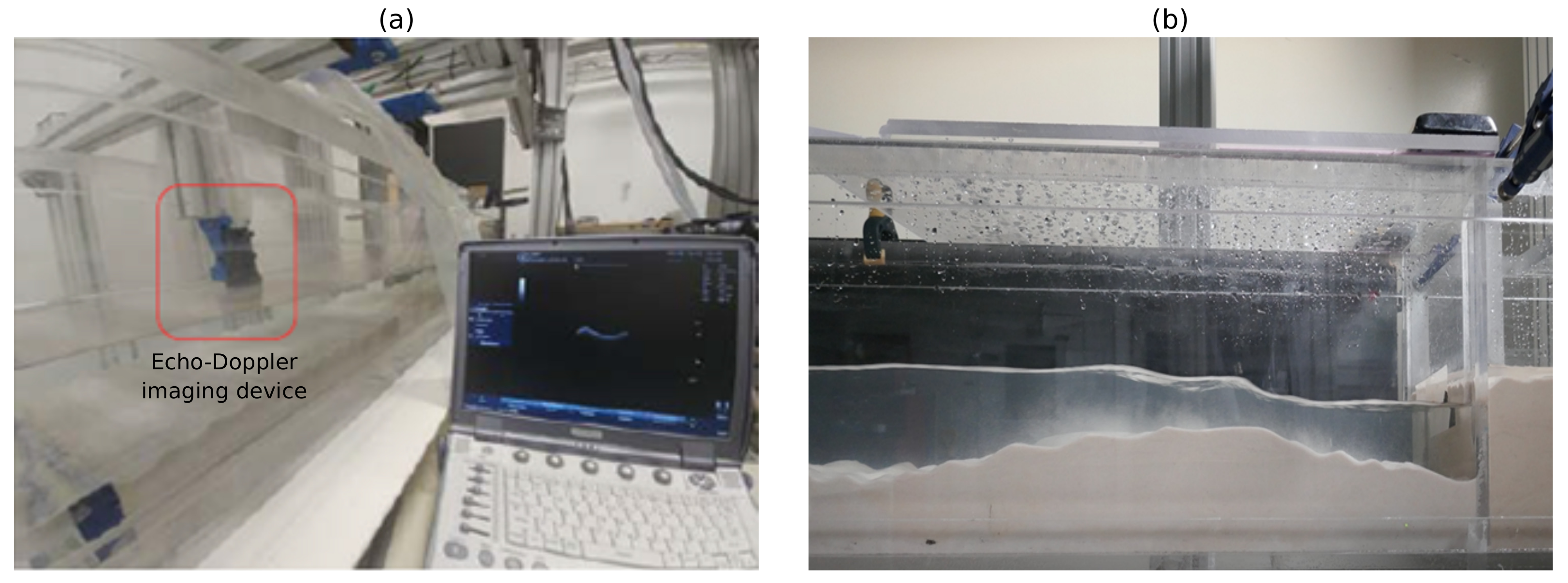
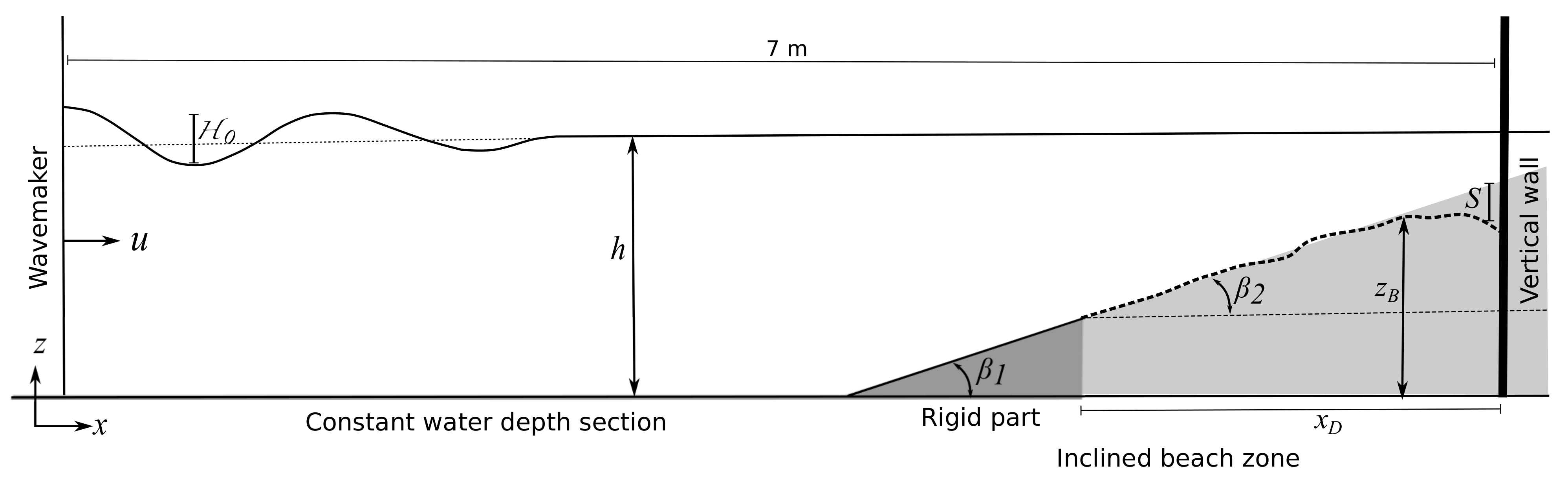
2. Laboratory Experiments
3. Mathematical Model
3.1. Hydrodynamic Model
3.2. Morphodynamic Model
3.3. Sand-Slide Model
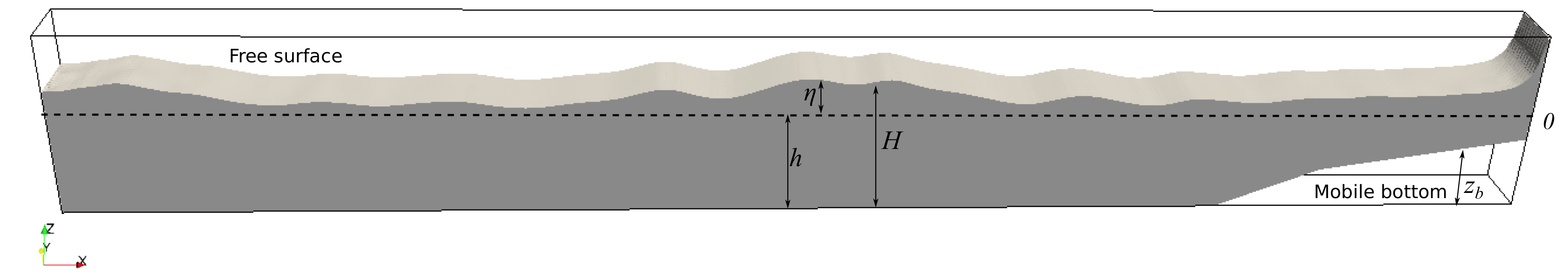
3.4. Equations in the -Coordinate System
4. Numerical Method
4.1. Projection Method
4.2. Time Integration
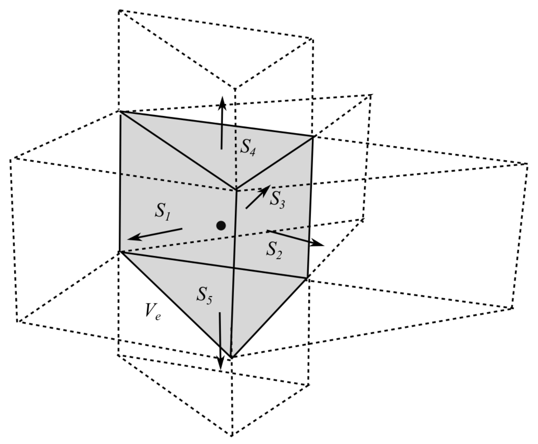
4.3. Unstructured Finite Volume Discretization
5. Numerical Results
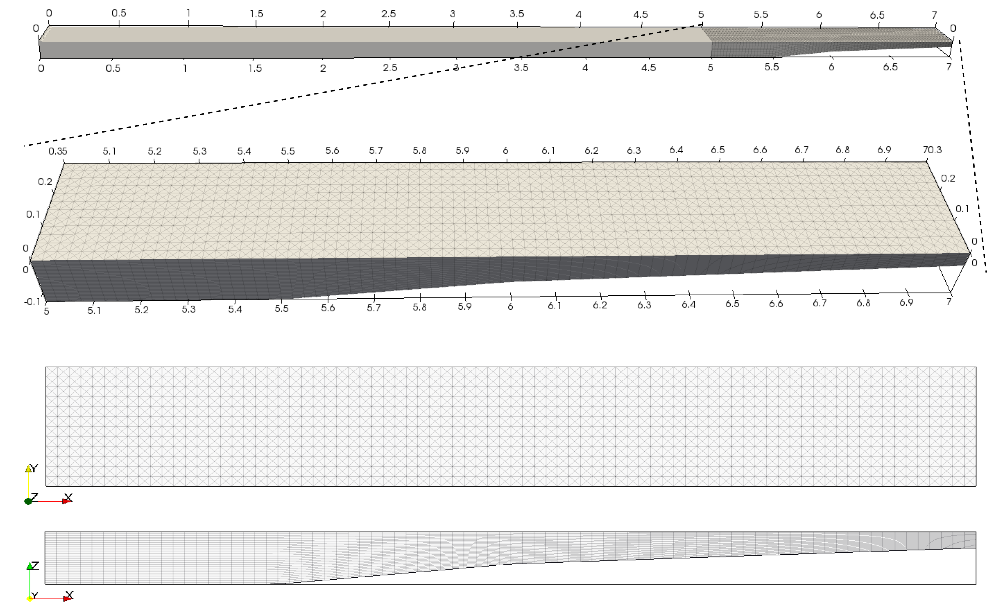
5.1. Numerical Setup
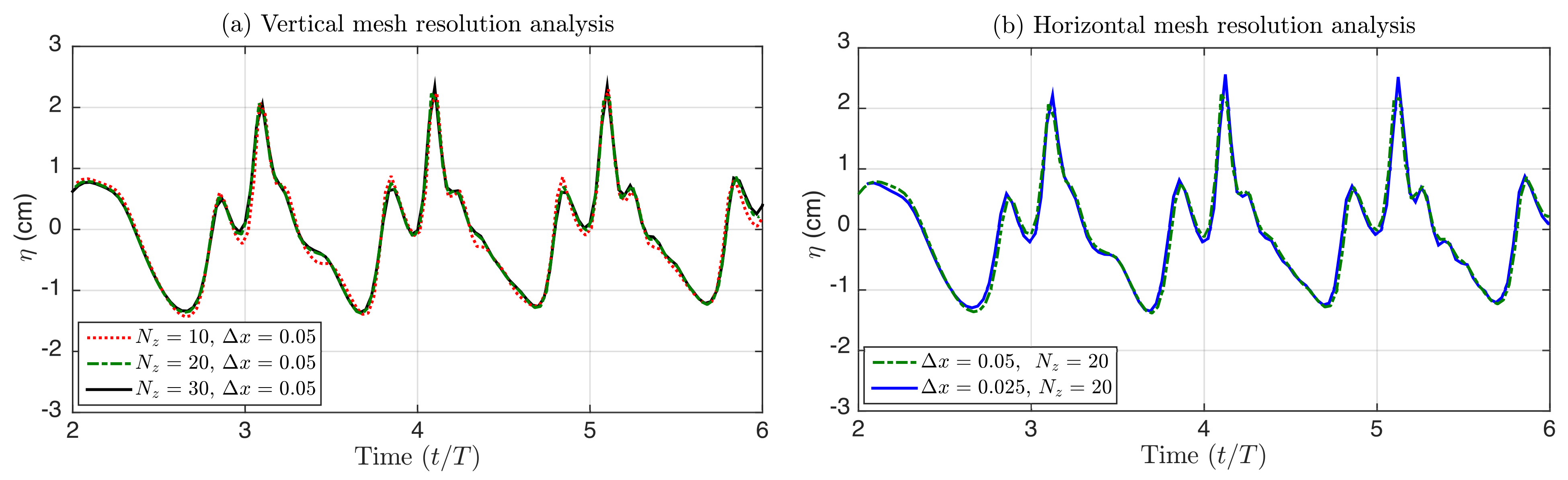
5.2. Grid Convergence Study
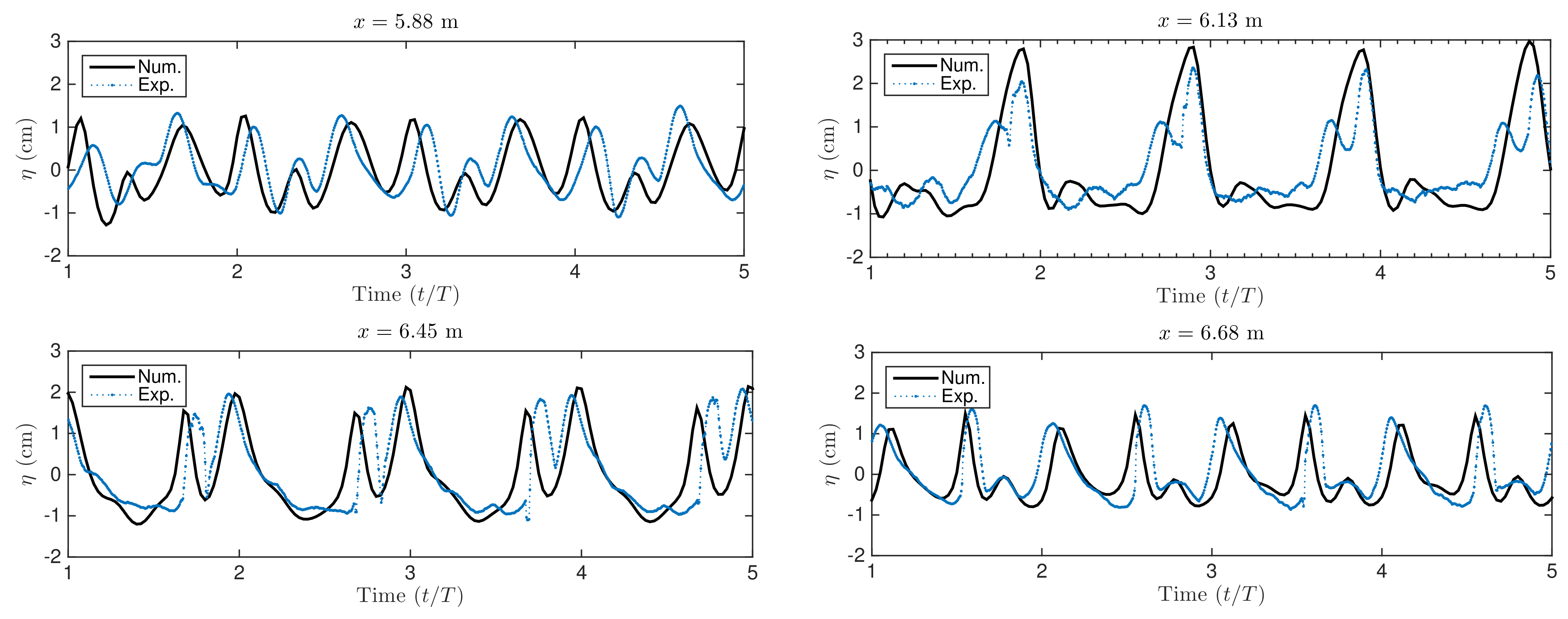
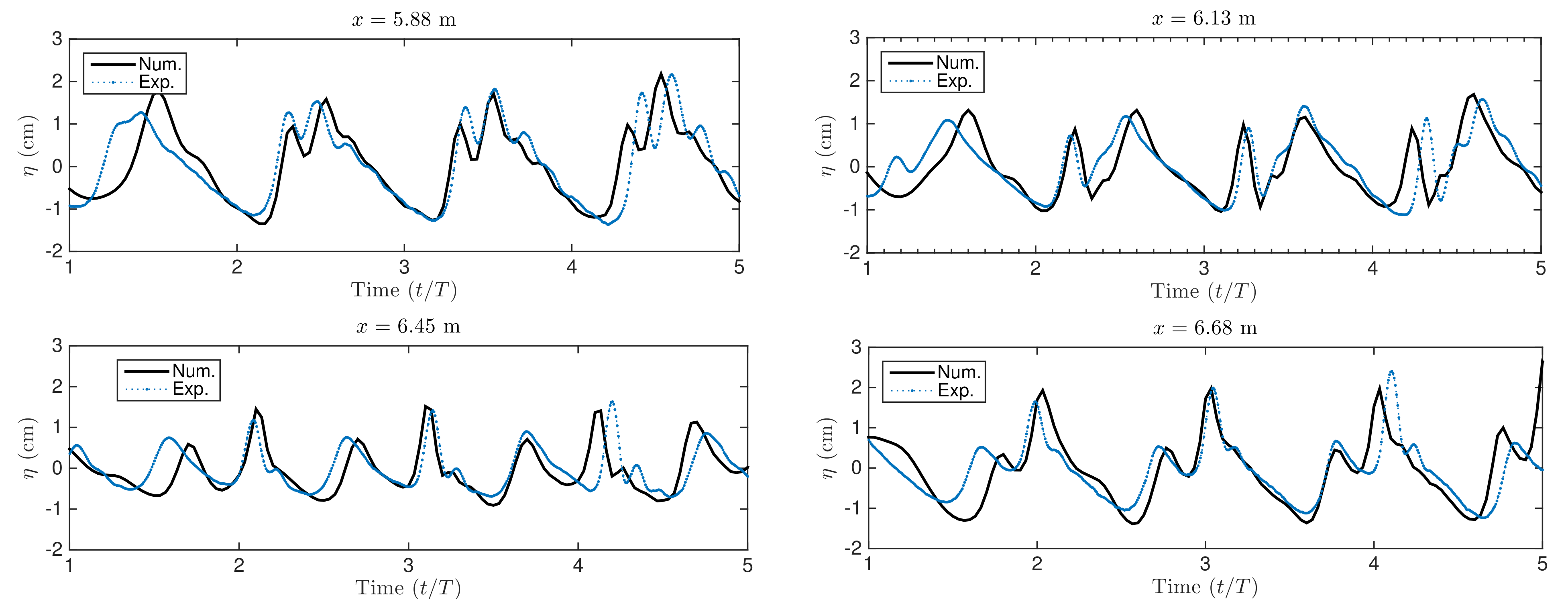
5.3. Wave Elevation
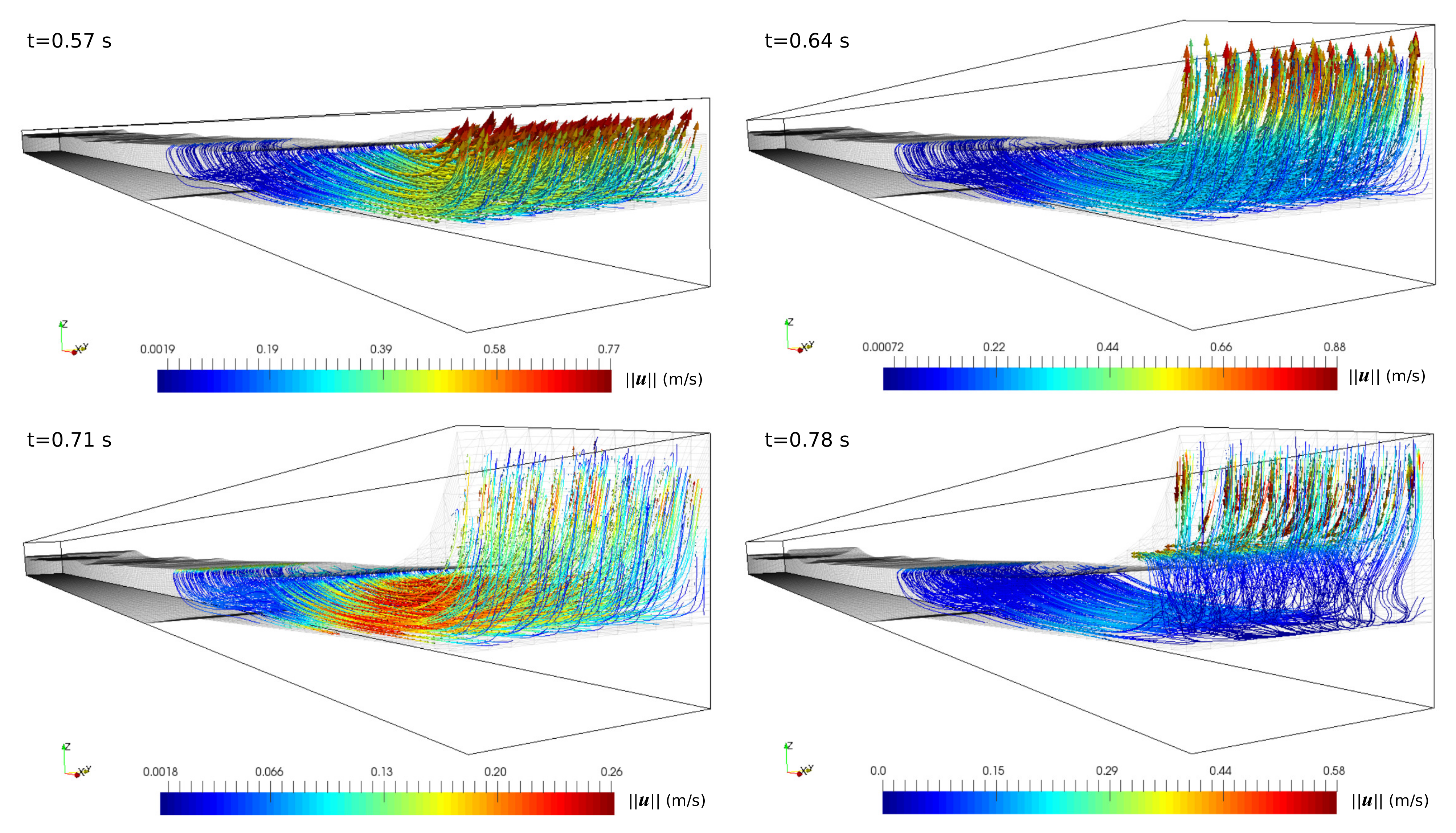
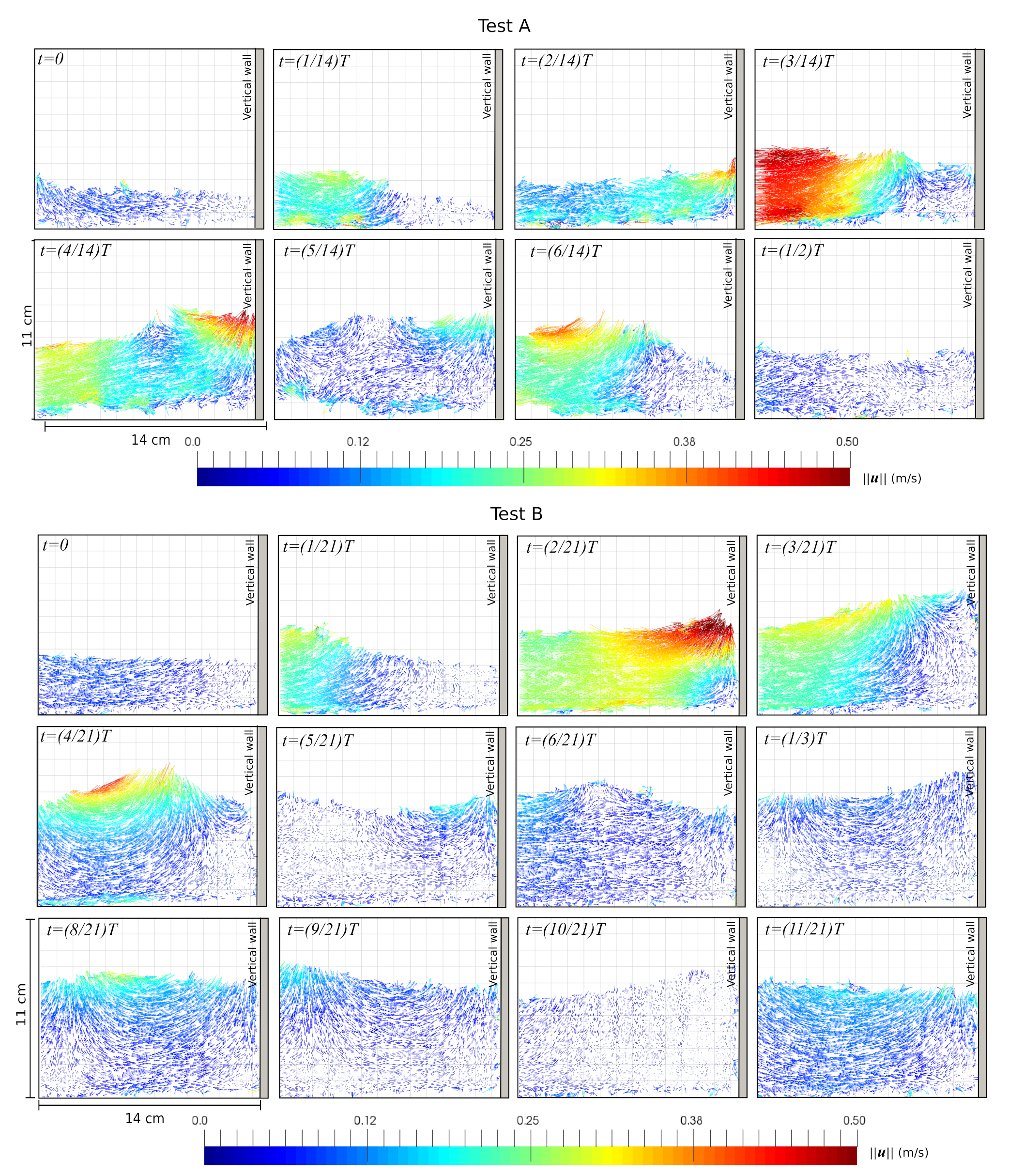
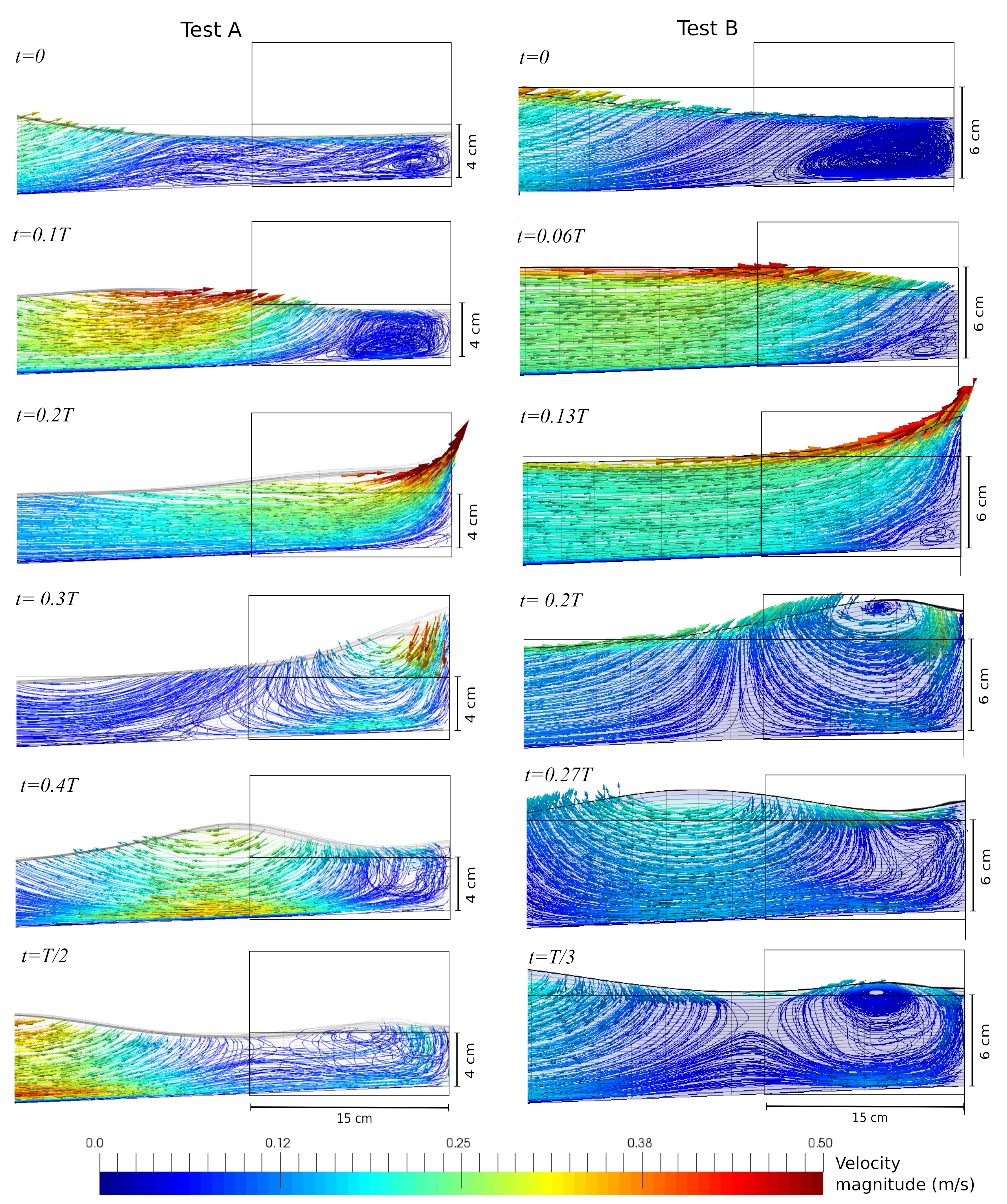
5.4. Velocity Field
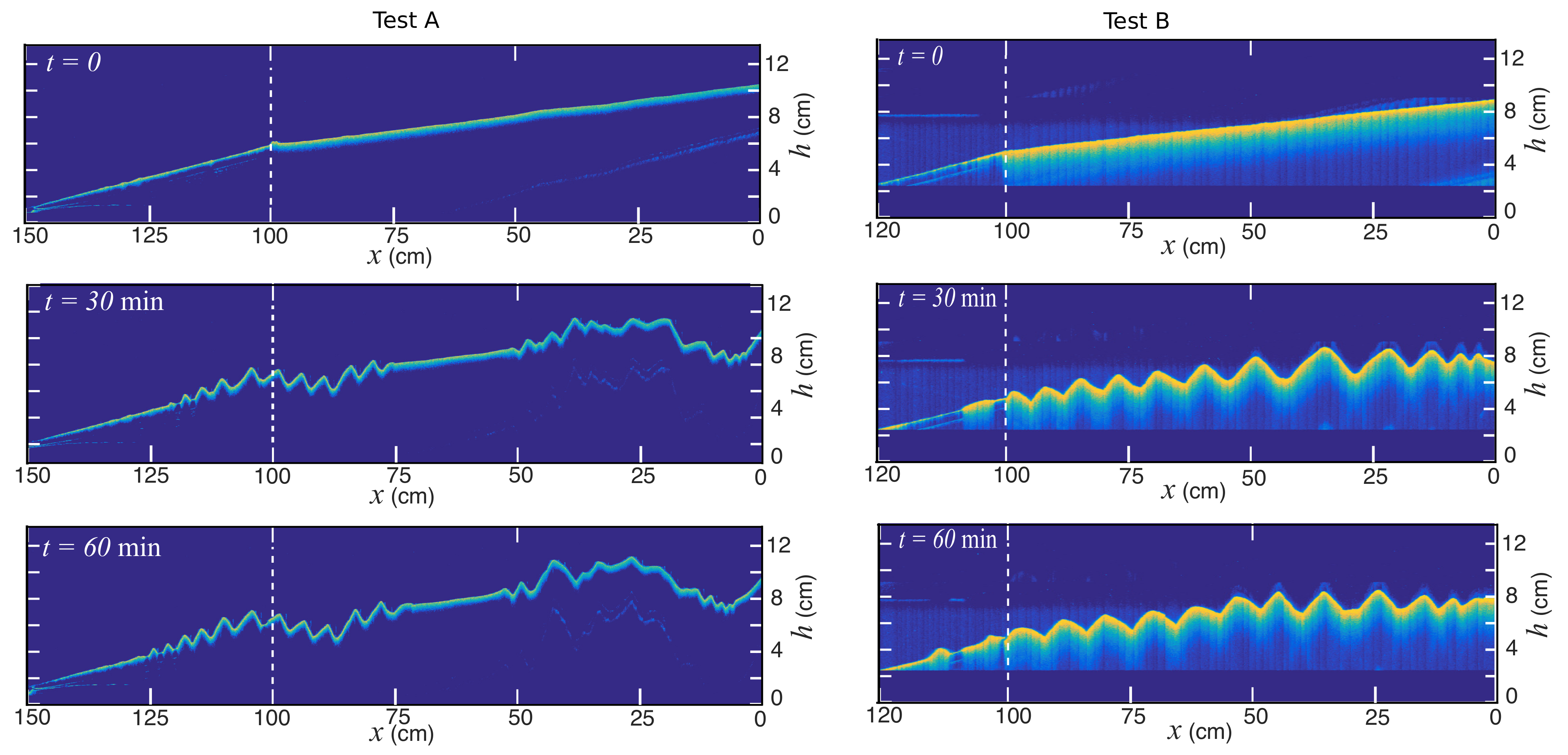
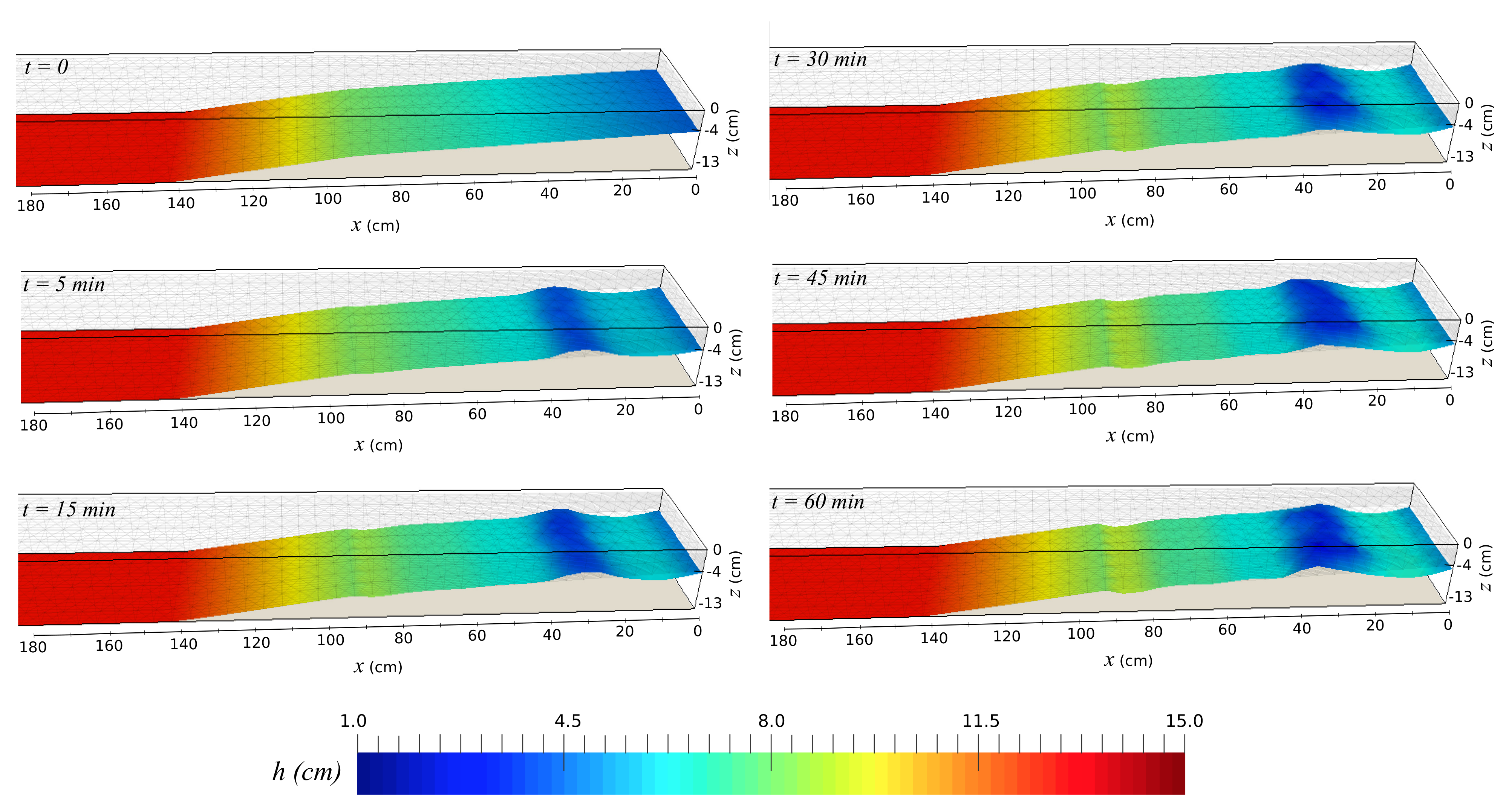
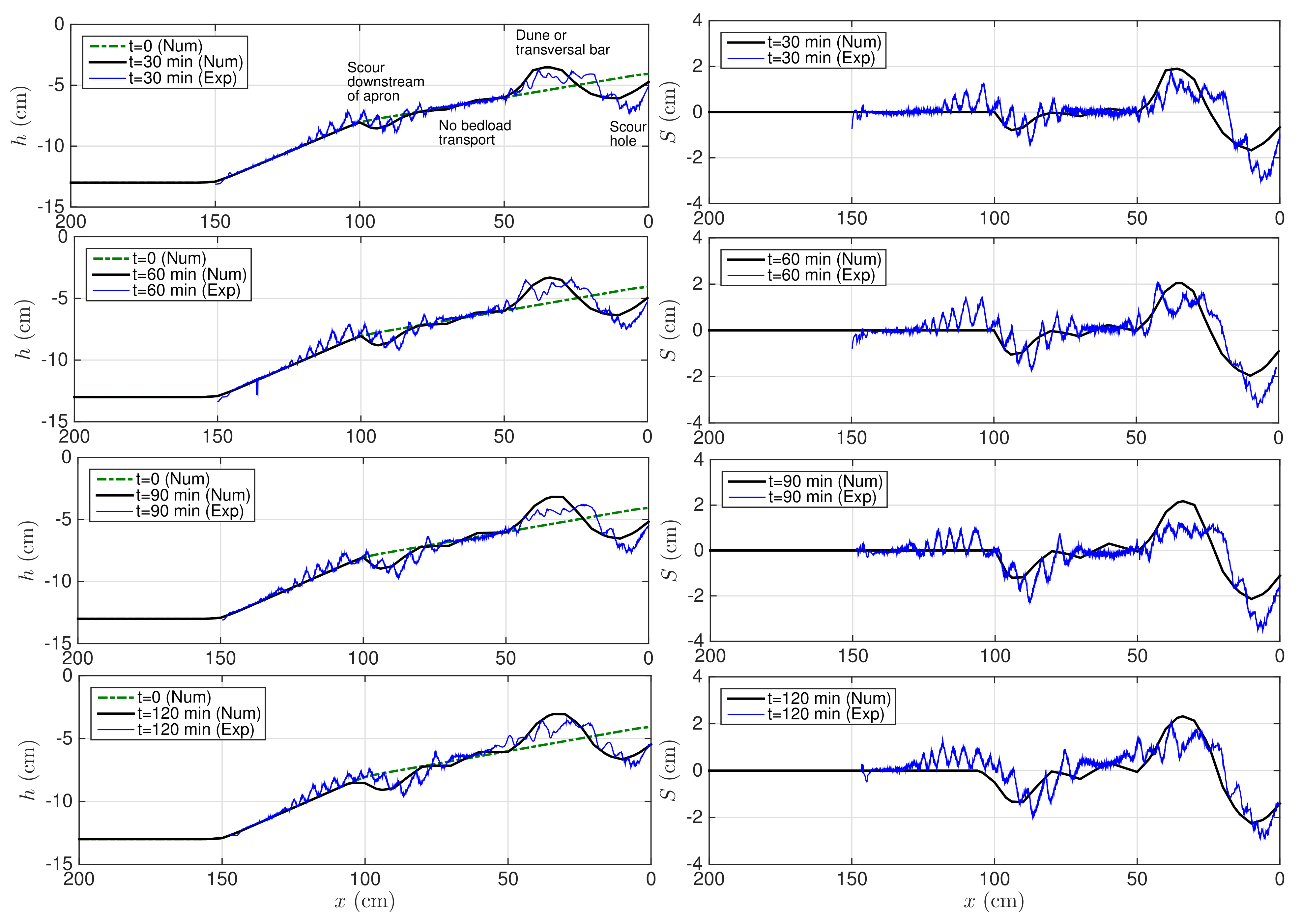
5.5. Seawall Scour
6. Conclusions
Author Contributions
Funding
Institutional Review Board Statement
Informed Consent Statement
Data Availability Statement
Acknowledgments
Conflicts of Interest
References
- Hugues, S.A. Physical models and laboratory techniques in coastal engineering, In Particular Section 5.4: Vertical Wall; World Scientific: Singapore, 1993; pp. 216–222. [Google Scholar]
- Hattori, M.; Kawamata, R. Experiments on restoration of beaches backed by seawalls. Coast. Eng. Jpn. 1977, 20, 55–68. [Google Scholar] [CrossRef]
- Sutherland, J.; Obhrai, C.; Whitehouse, R.J.S.; Pearce, A. Laboratory tests of scour at a seawall. In Proceedings of the 3rd International Conference on Scour and Erosion (ICSE), Amsterdam, The Netherlands, 1–3 November 2006. [Google Scholar]
- El-Bisy, M.S. Bed changes at toe of inclined seawalls. Ocean. Eng. 2007, 34, 510–517. [Google Scholar] [CrossRef]
- Pearson, J.M. Overtopping and Toe Scour at Vertical Seawalls, Coast, Marine Structures and Breakwaters; ICE: Atlanta, GA, USA, 2010; ISBN 978-0-7277-4131-8. [Google Scholar]
- Saitoh, T.; Kobayashi, N. Wave transformation and cross-shore sediment transport on sloping beach in front of vertical wall. J. Coast. Res. 2012, 128, 354–359. [Google Scholar] [CrossRef]
- Bang, D.P.V.; Marois, L.; Roches, M.D.; Daigle, L.F.; Letellier, P. Interactions entre un Mur de Protection Cotiere et le Transport sédimentaire: Affouillements Locaux au Pied et Abaissement Global de la Plage (Progress Report No. 3, Contract R829.1, Min. Transport; Institut National de la Recherche Scientifique: Quebec City, QC, Canada, 2020. [Google Scholar]
- Marois, L.; Stolle, J.; Bang, D.P.V. Processus d’affouillement au pied d’un mur vertical de protection cotiere. J. Natl. Génie Côtier 2020, 259–266. [Google Scholar] [CrossRef]
- Dally, W.R.; Dean, R.G. Suspended sediment transport and beach profile evolution. J. Waterw. Port Coast. Ocean. Eng. 1984, 110, 15–33. [Google Scholar] [CrossRef]
- Roelvink, J.A.; Stive, M.J.F. Bar-generating cross-shore flow mechanisms on a beach. J. Geophys. Res. Ocean. 1989, 94, 4785–4800. [Google Scholar] [CrossRef]
- McDougal, W.G.; Kraus, N.C.; Ajiwibowo, H. The effects of seawalls on the beach: Part II, numerical modeling of SUPERTANK seawall tests. J. Coast. Res. 1996, 12, 702–713. [Google Scholar]
- Gislason, K.; Fredsøe, J.; Sumer, B.M. Flow under standing waves. Part 2. Scour and deposition in front of breakwaters. Coast. Eng. 2009, 56, 363–370. [Google Scholar] [CrossRef]
- Myrhaug, D.; Ong, M.C. Random wave-induced scour at the trunk section of a breakwater. Coast. Eng. 2009, 56, 688–692. [Google Scholar] [CrossRef]
- Hajivalie, F.; Yeganeh-Bakhtiary, A.; Houshanghi, H.; Gotoh, H. Euler-Lagrange model for scour in front of vertical breakwater. Appl. Ocean. Res. 2012, 34, 96–106. [Google Scholar] [CrossRef]
- Zou, Q.; Peng, Z.; Lin, P. Effects of wave breaking and beach slope on toe scour in front of a vertical seawall. Coast. Eng. Proc. 2012, 1, 122. [Google Scholar] [CrossRef]
- Ahmad, N.; Bihs, H.; Chella, M.A.; Arntsen, A. CFD modelling of Arctic coastal erosion due to breaking waves. Int. J. Offshore Polar Eng. 2019, 29, 33–41. [Google Scholar] [CrossRef] [Green Version]
- Ahmad, N.; Bihs, H.; Myrhaug, D.; Kamath, A.; Arntsen, A. Numerical modeling of breaking wave induced seawall scour. Coast. Eng. 2019, 150, 108–120. [Google Scholar] [CrossRef]
- Zapata, M.U.; Zhang, W.; Bang, D.P.V.; Nguyen, K.D. A parallel second-order unstructured finite volume method for 3D free-surface flows using a σ-coordinate. Comput. Fluids 2019, 190, 15–29. [Google Scholar] [CrossRef]
- Zhang, W.; Zapata, M.U.; Bai, X.; Pham-Van-Bang, D.; Nguyen, K.D. Three-dimensional simulation of horseshoe vortex and local scour around a vertical cylinder using an unstructured finite-volume technique. Int. J. Sediment Res. 2020, 35, 295–306. [Google Scholar] [CrossRef]
- Phillips, N.A. A coordinate system having some special advantages for numerical forecasting. J. Meteor. 1957, 14, 184–185. [Google Scholar] [CrossRef] [Green Version]
- Chen, C.; Liu, H. An unstructured Grid, Finite Volume, Three-Dimensional, Primitive Equations Ocean Model: Application to Coastal Ocean and Estuaries. J. Atmos. Ocean. Technol. 2003, 20, 159–186. [Google Scholar] [CrossRef]
- Liu, X.; Mohammadian, A.; Sedano, J.A.I. Three-dimensional modeling of non-hydrostatic free-surface flows on unstructured grids. Int. J. Numer. Meth. Fluids 2016, 82, 130–147. [Google Scholar] [CrossRef]
- van Rijn, L.C. Sediment transport, Part I: Bed load transport. J. Hydraul. Eng. 1984, 110, 1431–1456. [Google Scholar] [CrossRef] [Green Version]
- Chorin, A.J. Numerical solution of the Navier—Stokes equations. Math. Comp. 1968, 22, 745–762. [Google Scholar] [CrossRef]
- Temam, R. Sur l’approximation des équations de Navier-Stokes par la méthode des pas fractionnaires (II). Arch. Ration. Mech. Anal. 1967, 26, 367–380. [Google Scholar] [CrossRef]
- Rhie, C.M.; Chow, W.L. Numerical study of the turbulent flow past an airfoil with trailing edge separation. AIAA J. 1983, 21, 1525–1532. [Google Scholar] [CrossRef]
- Grasso, F.; Michallet, H.; Barthélemy, E.; Certain, R. Physical modeling of intermediate cross-shore beach morphology: Transients and equilibrium states. J. Geophys. Res. Ocean. 2009, 114, C9. [Google Scholar] [CrossRef] [Green Version]
- Nikuradse, J. Laws of Flow in Rough Pipes; VDI Forschungsheft: Washington, DC, USA, 1933. [Google Scholar]
- Roulund, A.; Sumer, B.M.; Fredsøe, J.; Michelsen, J. Numerical and experimental investigation of flow and scour around a circular pile. J. Fluid Mech. 2005, 534, 351–401. [Google Scholar] [CrossRef]
- Khosronejad, A.; Kang, S.; Borazjani, I.; Sotiropoulos, F. Curvilinear immersed boundary method for simulating coupled flow and bed morphodynamic interactions due to sediment transport phenomena. Adv. Water Resour. 2011, 34, 829–843. [Google Scholar] [CrossRef]
- Khosronejad, A.; Kang, S.; Sotiropoulos, F. Experimental and computational investigation of local scour around bridge piers. Adv. Water Resour. 2012, 37, 73–85. [Google Scholar] [CrossRef]
- Lin, P.; Li, C.W. A σ-coordinate three-dimensional numerical model for surface wave propagation. Int. J. Numer. Methods Fluid 2002, 38, 1045–1068. [Google Scholar] [CrossRef]
- Kim, D.; Choi, H. A second-order time-accurate finite volume method for unsteady incompressible flow on hybrid unstructured grids. J. Comput. Phys. 2000, 162, 411–428. [Google Scholar] [CrossRef]
- Barth, T.; Jespersen, D.C. The design and application of upwind schemes on unstructured meshes. In Proceedings of the 27th Aerospace Sciences Meeting, Reno, NV, USA, 9–12 January 1989; p. 366. [Google Scholar]
- Vidović, D.; Segal, A.; Wesseling, P. A superlinearly convergent Mach-uniform finite volume method for the Euler equations on staggered unstructured grids. J. Comput. Phys. 2006, 217, 277–294. [Google Scholar] [CrossRef]
- Zapata, M.U.; Bang, D.P.V.; Nguyen, K.D. An unstructured finite volume technique for the 3D Poisson equation on arbitrary geometry using a σ-coordinate system. Int. J. Numer. Meth. Fluids 2014, 76, 611–631. [Google Scholar] [CrossRef]
- Zhang, W.; Zapata, M.U.; Bai, X.; Bang, D.P.V.; Nguyen, K.D. An unstructured finite volume method based on the projection method combined momentum interpolation with a central scheme for three-dimensional nonhydrostatic turbulent flows. Eur. J. Mech.-B/Fluids 2020, 84, 164–185. [Google Scholar] [CrossRef]
- Oumeraci, H.; Klammer, P.; Partenscky, H.W. Classification of breaking wave loads on vertical structures. J. Waterw. Port Coast. Ocean Eng. 1993, 119, 381–397. [Google Scholar] [CrossRef]
- Hasselmann, K.; Munk, W.; MacDonald, G. Bispectrum of Ocean Waves; Rosenblatt, M., Ed.; Time Series Analysis; JohnWiley: New York, NY, USA, 1963. [Google Scholar]
- Bertin, X.; de Bakker, A.; van Dongeren, A.; Coco, G.; André, G.; Ardhuin, F.; Bonneton, P.; Bouchette, F.; Castelle, B.; Crawford, W.C.; et al. Infragravity waves: From driving mechanisms to impacts. Earth Sci. Rev. 2018, 177, 774–799. [Google Scholar] [CrossRef] [Green Version]
- Lin, C.-Y.; Huang, C.-J. Decomposition of incident and reflected higher harmonic waves using four wave gauges. Coast. Eng. 2004, 51, 395–406. [Google Scholar] [CrossRef]
- Amoudry, L.O.; Liu, P.L.-F. Two-dimensional, two-phase granular sediment transport model with applications to scouring downstream of an apron. Coast. Eng. 2009, 56, 693–702. [Google Scholar] [CrossRef]


| Name | (m) | (cm) | T (s) | L (m) | h (cm) | (cm) | (cm) | ||
|---|---|---|---|---|---|---|---|---|---|
| Test A | 216 | 1.7 | 2 | 2.209 | 13 | 4 | 1/10 | 1/25 | 100 |
| Test B | 700 | 1.6 | 3 | 2.365 | 15 | 6 | 1/10 | 1/25 | 100 |
| Sub-Divisions | Vertices | Cells | Prisms | |||
|---|---|---|---|---|---|---|
| Mesh 1 | 0.05 m | 20 | 1827 | 3360 | 62,200 | |
| Mesh 2 | 0.025 m | 20 | 7013 | 13,440 | 268,800 |
Publisher’s Note: MDPI stays neutral with regard to jurisdictional claims in published maps and institutional affiliations. |
© 2021 by the authors. Licensee MDPI, Basel, Switzerland. This article is an open access article distributed under the terms and conditions of the Creative Commons Attribution (CC BY) license (https://creativecommons.org/licenses/by/4.0/).
Share and Cite
Uh Zapata, M.; Pham Van Bang, D.; Nguyen, K.D. Unstructured Finite-Volume Model of Sediment Scouring Due to Wave Impact on Vertical Seawalls. J. Mar. Sci. Eng. 2021, 9, 1440. https://doi.org/10.3390/jmse9121440
Uh Zapata M, Pham Van Bang D, Nguyen KD. Unstructured Finite-Volume Model of Sediment Scouring Due to Wave Impact on Vertical Seawalls. Journal of Marine Science and Engineering. 2021; 9(12):1440. https://doi.org/10.3390/jmse9121440
Chicago/Turabian StyleUh Zapata, Miguel, Damien Pham Van Bang, and Kim Dan Nguyen. 2021. "Unstructured Finite-Volume Model of Sediment Scouring Due to Wave Impact on Vertical Seawalls" Journal of Marine Science and Engineering 9, no. 12: 1440. https://doi.org/10.3390/jmse9121440