Multi-Objective Optimisation of the Benchmark Wind Farm Layout Problem

Abstract

Wind farm layout optimisation has become a very challenging and widespread problem in recent years. In many publications, the main goal is to achieve the maximum power output and minimum wind farm cost. This may be accomplished by applying single or multi-objective optimisation techniques. In this paper, we apply a single objective hill-climbing algorithm (HCA) and three multi-objective evolutionary algorithms (NSGA-II, SPEA2 and PESA-II) to a well-known benchmark optimisation problem proposed by Mosetti et al., which includes three different wind scenarios. We achieved better results by applying single- and multi-objective algorithms. Furthermore, we showed that the best performing multi-objective algorithm was NSGA-II. Finally, an extensive comparison of the results of past publications is made.

1. Introduction

As the transformation from fossil fuels to renewable energy sources gains momentum, minimising the cost while maximising the power output of renewable energy sources is becoming more critical than ever. It has been shown that the power extracted from onshore and offshore wind farms could cover the world’s electricity demand seven times over, assuming that only 20% of wind potential was used. This can be achieved with wind farms that are within 50 nautical miles (92.6 km) and water depths that do not exceed 200 m [1]. These restrictions could be eased, and possibly more power could be generated. According to the UK government, offshore wind farms will generate enough energy to power every house in the United Kingdom by 2030.

In order to obtain wind farms providing high energy yields at a low cost, optimisation can be employed to ensure that wind turbines are deployed efficiently and productively. The general idea is that if we place wind turbines too close to each other, then the efficiency of the wind farm could drop by up to 30% [2]. This is because there is a naturally occurring interaction between wind turbines known as the wake effect. Therefore, to reduce the wake effect, we can optimise the positioning of the wind turbines on the farm. This was first accomplished by Mosetti et al. [3] in 1994, where they minimised the cost to power ratio under three different wind scenarios using a genetic algorithm.

The aim of this work is to examine the performance of various optimisation algorithms when applied to the wind farm layout problem and to benchmark against other existing approaches of solving similar problems. Given that, the problem posed by Mosetti et al. is an ideal case study as it has been used widely. We acknowledge that other, newer problem formulations capture different aspects of the problem, and the results we demonstrate herein are intended to form a basis for further exploration of optimisation on those specific problems. The aim of this work is not to advance the state of the art in wind farm layout, but to explore the characteristics of different optimisation strategies and to disseminate knowledge that can be of use to engineers when optimising their specific wind farm layout problem formulations. The Mosetti et al. problem is still widely used in the literature. For example, Javadi et al. [4] compared the performance of Monte Carlo simulation with that of genetic algorithms using the Mosetti et al. formulation. Work by Moreno et al. [5] conducted a similar study to that undertaken herein, though with a continuous problem representation rather than a discrete one—for the purposes of benchmarking, the more traditional discrete representation has been retained in this work. Yang et al. [6] used the wind farm problem proposed by Mosetti et al. to benchmark the effect of using different analytical wake models in a similar methodological approach to our own, in which we are comparing the efficacy of different optimisers.

A large number of authors followed this idea and implemented varying algorithms to solve the same problem. In many publications, the initial conditions formulated by Mosetti et al. [3] were varied, including applying different wake models, changing the grid size, implementing different types of wind turbines and redefining the cost of wind farms. Thus, feasible comparisons of these newer works with that of Mosetti et al. [3] are limited. Other works adopted identical conditions to those proposed by Mosetti et al. and used genetic algorithms [7,8,9,10], particle swarm optimisation [11], mixed integer programming [12,13] and simulated annealing [14], for example.

Multi-objective optimisation of wind farm layouts has also been performed, as already mentioned. For example, Şişbot et al. [15] minimised the cost and maximised the power output of the wind farm on Gökceada Island using a MOGA [16]. Such algorithms use a population of candidate solutions and evolve them toward the optimal trade-off between problem objectives using a fitness-based selection mechanism. Solutions with the best objective function values are retained and used as a basis for generating new candidate solutions in the next generation. This process continues until some limit is reached, typically when a fixed budget of function evaluations is exhausted. Examples of such algorithms that have been employed in this field are SPEA2 [17], NSGA-II [18], PESA-II [19] and IBEA [20]. Kusiak et al. [21] applied SPEA2 [17] to optimise the position of the wind turbines under constraints (wind farm radius and wind turbine distance). Tran et al. [22] maximised the power output and minimised the length of the cables and wind farm area using three evolutionary algorithms: IBEA [20], NSGA-II [18] and SPEA2 [17]. Finally, Rodrigues et al. [23] compared the performance of the NSGA-II [18] and MOGOMEA [23] by maximising two objective functions: efficiency and power output of the wind farm.

A careful review of the existing works listed above and others reveals some methodological problems. For example, Marmidis et al. [24] performed optimisation of wind farm layouts using a Monte Carlo simulation method. In an ideal case scenario, the efficiency of the wind farm is 100% (this refers to the situation where the wake effect does not occur). However, it was shown by Mittal [25] that the efficiency of the optimised wind farm layout, found by Marmadis et al., was above 100%, which is impossible. In another example, Grady et al. 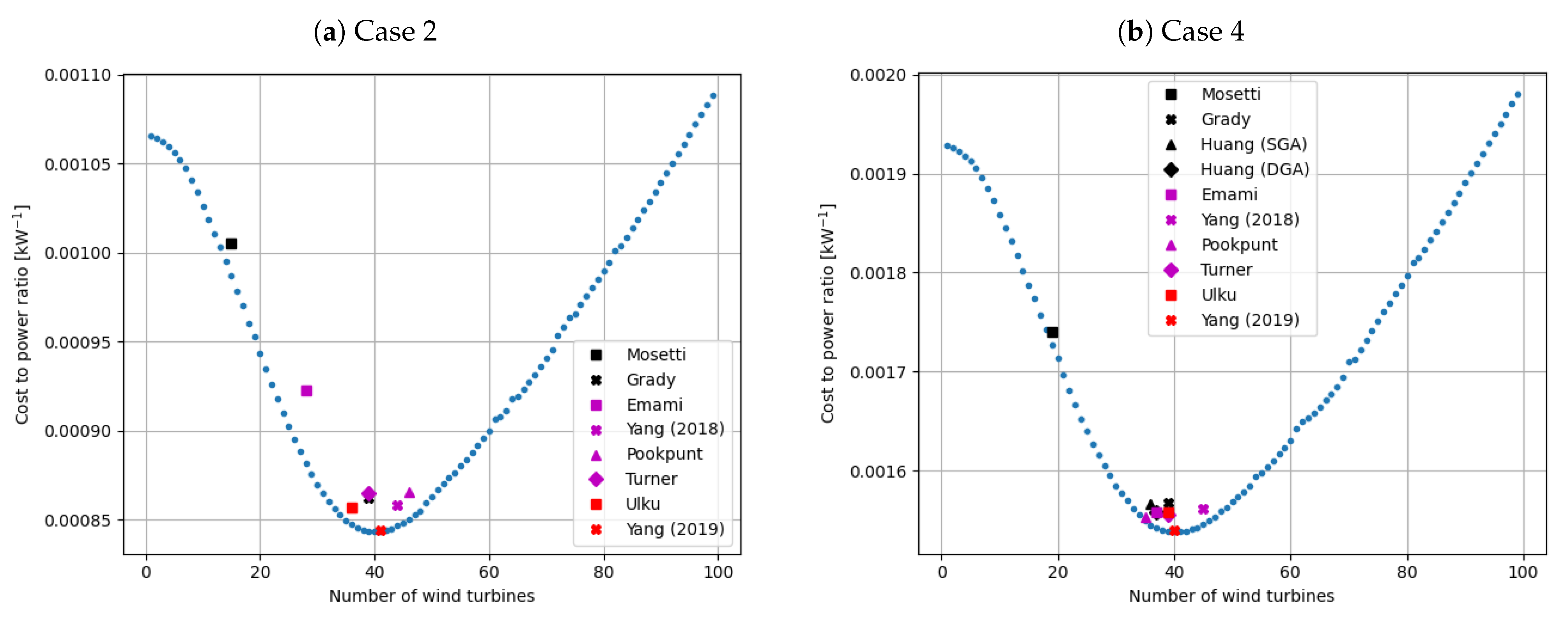[7] applied a genetic algorithm and found an optimal solution for the simplest case scenario (more about this later). The same wind farm layout was reported by Ulku et al. [13] and Turner et al. [12], but the calculated power output of the wind farm was different by circa 13% and 4%, respectively. Unfortunately, such a lack of consistency is apparent in many publications, and an accurate comparison of results is challenging. To overcome this problem, we adopted and recalculated reported wind farm layouts into our model.

In this paper, we perform a single and multi-objective optimisation of the problem introduced by Mosetti et al. [3]. In the single objective optimisation part, we implement a simple, well-known hill-climbing algorithm (HCA). We aim to demonstrate that using a simple algorithm can produce the same or even better results, as there is no need for using a more sophisticated approach. Furthermore, the way we apply the HCA allows us to transform from single- to multi-objective optimisation. We apply to the problem three algorithms (NSGA-II, SPEA2 and PESA-II) and compare their performance. Finally, we choose the best performing algorithm and compare it with an HCA.

The remainder of this paper is organised as follows. In the next section, we will explain the framework proposed by Mosetti et al. [3]. It involves wake modelling and calculating wind farm power output and cost, wind farm geometry, and wind distribution. In the third section, we will focus on single- and multi-objective optimisation algorithms. In the following section, a comparison of the results will be performed, and in the last section, we will provide the reader with our conclusions.

2. Wind Farm Modelling

There is huge flexibility in wind farm modelling: the wind farm layout can be either discrete (the possible locations of the wind turbines are predefined [3,7,8,9,10,11,12,13,14]) or continuous (there are no restrictions as to where wind turbines can be placed [6,21,26]). One or more types of a wind turbine can be installed on the same farm [27], different wind distributions (mean value [3,6,7,8,9,10,11,12,13,14], Weibull distribution [21,28] or real data [28,29]) can be applied and cost of the wind farm can just be a function of the number of wind turbines [3,6,7,8,9,10,11,12,13,14], or more sophisticated models can be incorporated (for example, initial capital cost, replacement cost, operational and maintenance [30]). The most important factor, however, is the wake model. If we are interested in working with highly precise predictions of wind farm power output, we likely need to employ sophisticated wake models with high precision but a long computational time. On the other hand, if we are more focused on optimisation, we need to reach for simple wake models that allow us to perform large numbers of computations within a reasonable time.

In this paper, we are interested in optimisation and a results comparison of previous works, and therefore, all the following wind farm characteristics were adopted from Mosetti et al. [3], all of which will be fully described in the following subsections:

• Discrete wind farm layout (100 possible locations for wind turbines).
• Jensen wake model.
• Only one type of wind turbine.
• Simplified cost of the wind farm (the cost of the wind farm solely depends on the number of wind turbines).
• Constant thrust coefficient of wind turbines (simplifying the calculation of wind farm power output).
• Three wind distributions.

2.1. Single Wake Model

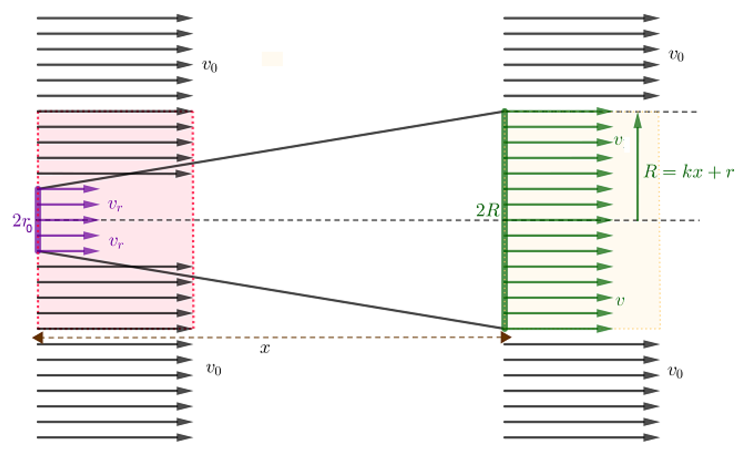
Various different wake models have been proposed [2] that described the reduction of kinetic energy when the wind turbine rotor is hit. Jensen’s wake model (Figure 1) is the simplest of them. It was first introduced by Jensen [31] in 1983, and in 1986, the Katic–Jensen [32] model was formulated. Despite the age of this model, it is still widely used in the literature [4,6,33]. Furthermore, the comprehensive comparative analysis of a number of newer analytical wake models revealed that the Jensen wake model provides ‘…acceptable accuracy (maximum percentage deviation 9%)’ [33]. Given that the aim of this work is to benchmark and compare to existing results published in the literature, we have retained the Katic–Jensen wake model, as was used in those works, and which is formulated as

$$v=v_0\left[1-\frac{\left(1-\sqrt{1-C_t}\right)}{{\left(1+\frac{kx}{r}\right)}^2}\right],$$

(1)

where v is the wind velocity behind the rotor for a given distance between wind turbines x, thrust coefficient $C_t$, initial wind velocity $v_0$ and wake decay constant k which is calculated from

$$k=\frac{0.5}{ln\left(\frac{z}{z_0}\right)},$$

(2)

where z is the height of the wind turbine, and $z_0$ is a roughness of the terrain. The radius of the wake region immediately behind the rotor r is calculated from

$$r=r_0\sqrt{\frac{1-a}{1-2a}},$$

(3)

where the radius of the rotor is denoted by $r_0$, and a is the axial induction factor dependent on the thrust coefficient $C_t$:

$$a=\frac{1}{2}\left(1-\sqrt{1-C_t}\right).$$

(4)

Finally, the radius of the wake region R is found by

$$R=kx+r.$$

(5)

The simplicity of this model arises from the fact that the only variables are initial wind velocity $v_0$ and distance between wind turbines x. All the other factors, gathered in

Table 1. Properties of the wind farm proposed by Mosetti et al.

Thrust coefficient ($C_t$)	0.88
Axial induction factor (a)	0.3267949192
Rotor radius ($r_0$)	20 m
Rotor diameter (D)	40 m
Height of the wind turbine (z)	60 m
Roughness of the terrain ($z_0$)	0.03 m
Wake decay factor (k)	0.0943695829
Air density ($\rho$)	1.225 kg/m${}^3$
Power coefficient ($C_p$)	0.39
Swept area (A)	1256.64 m${}^2$

and proposed by Mosetti et al., are considered constant.

2.2. Multiple Wake Model and Partial Wake Effect

In large wind farms, there is a chance that wind turbines are in the wake region of more than one wind turbine. In order to calculate the wind deficit, the sum of squares method was proposed by Katic et al. [32]:

$${\left(1-\frac{v}{v_0}\right)}^2=\sum _{i=1}^N{\left(1-\frac{v_i}{v_0}\right)}^2,$$

(6)

where N denotes the number of wind turbines in the wake region. Furthermore, a wind turbine can also be only partially in the wake region of another wind turbine(s). To reflect this concept, wind velocity is calculated from

$$v_i=v_0\left[1-\frac{\left(1-\sqrt{1-C_t}\right)}{{\left(1+\frac{kx}{r}\right)}^2}\left(\frac{A_0}{A_i}\right)\right],$$

(7)

where $A_i$ is the area swept by the rotor of the ith wind turbine, and $A_0$ is the overlapped area between rotor and wake areas. Equations (6) and (7) formed the foundation to our analysis and were implemented in this paper.

2.3. Wind Farm Power Output

Only one type of wind turbine was considered, and its properties were gathered in Table 1. The power output of the wind farm was calculated from

$$P=\sum _{i=1}^N\frac{1}{2}\rho A{C}_p{v}_i^3\approx \sum _{i=1}^{N}0.3v_i^3,$$

(8)

where N is the number of wind turbines, $\rho$ denotes air density, A is the area swept by the rotor, $C_p$ is the power coefficient and $v_i$ is the wind velocity at the location of the ith wind turbine.

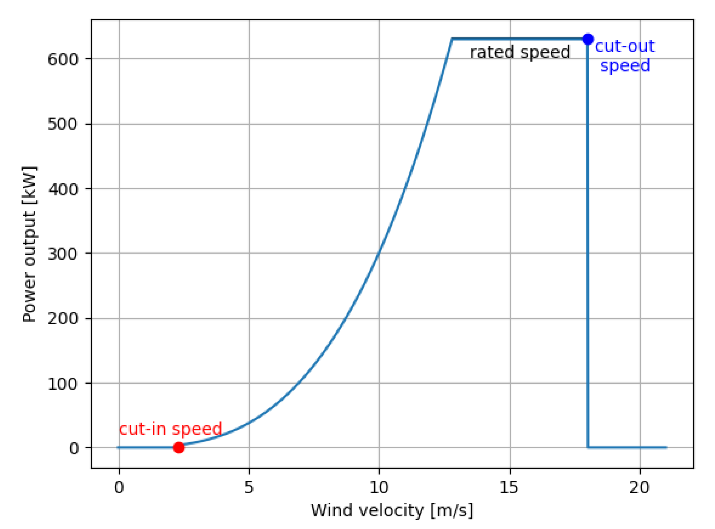
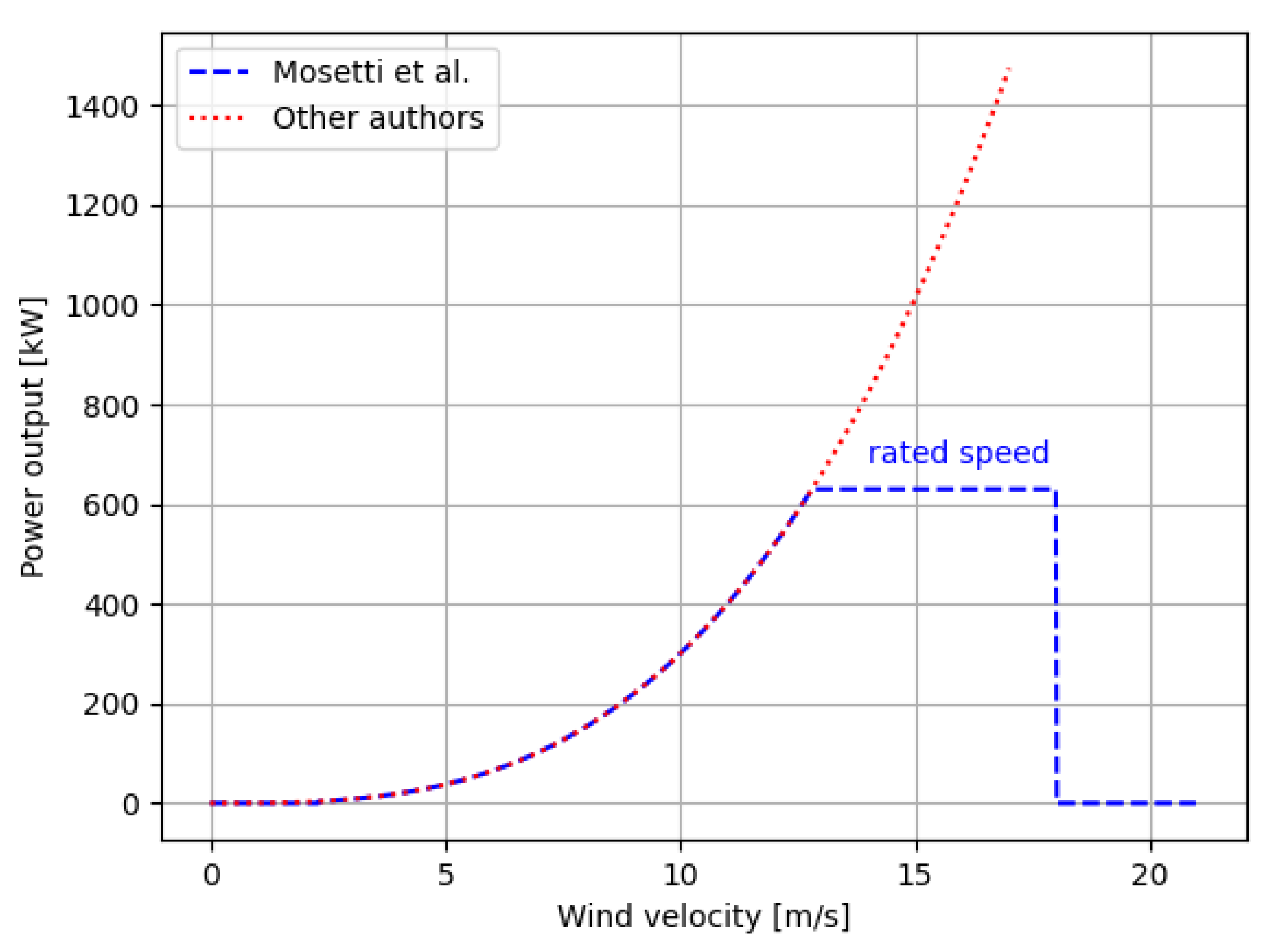
Equation (8) should only by applied if the wind velocity is between 2.3 m/s (cut-in speed) and 12.8 m/s (rated speed) (Figure 2). When wind velocity is between 12.8 m/s and 18 m/s (rated speed), the power output is constant and equal to 630 kW. For all other wind velocities, the power output should be equal to zero kilowatts. Therefore, Equation (8) needs to be reformulated:

$$P=\sum _{i=1}^N{P}_i,$$

(9)

where

$$P_i=\left\{\begin{array}{cc}0.3v_i^3\hfill & \mathrm{for}2.3⩽v_i⩽12.8\hfill \\ 630\hfill & \mathrm{for}12.8<v_i⩽18\hfill \\ 0\hfill & \mathrm{otherwise}.\hfill \end{array}\right.$$

It should be noted at this point that most researchers did not include Equation (9) in their work. This leads to some significant differences in results (e.g., Table 3).

2.4. Wind Farm Efficiency

The efficiency of the wind farm is defined as the sum over all wind turbines of their powers $P_i$ (as above) divided by each turbine’s maximum power output.

2.5. Wind Farm Cost

Mosetti et al. modelled wind farm cost by a function of the number of wind turbines, N:

$$\mathrm{cost}=N\left(\frac{2}{3}+\frac{1}{3}{e}^{-0.0017N^2}\right).$$

(10)

It was assumed that the (dimensionless) cost of one wind turbine is almost equal to one. For large wind farms, the cost reduction is asymptotically equal to 1/3. This approach was based on the concept that the cost for large numbers of wind turbines should be reduced.

2.6. Wind Farm Layout

A square 2000 × 2000 m grid with 100 equal-sized square cells for wind turbine placement was proposed [3]. Each wind turbine can occupy the centre of a single 200 × 200 m cell. Consequently, the minimum distance between two wind turbines is 200 m or five times the rotor diameter (5D). This is very important, since the Katic–Jensen wake model is applicable for far wakes only. A far wake is a minimum distance between two wind turbines equal to at least three to four rotor diameters [2].

2.7. Wind Distributions

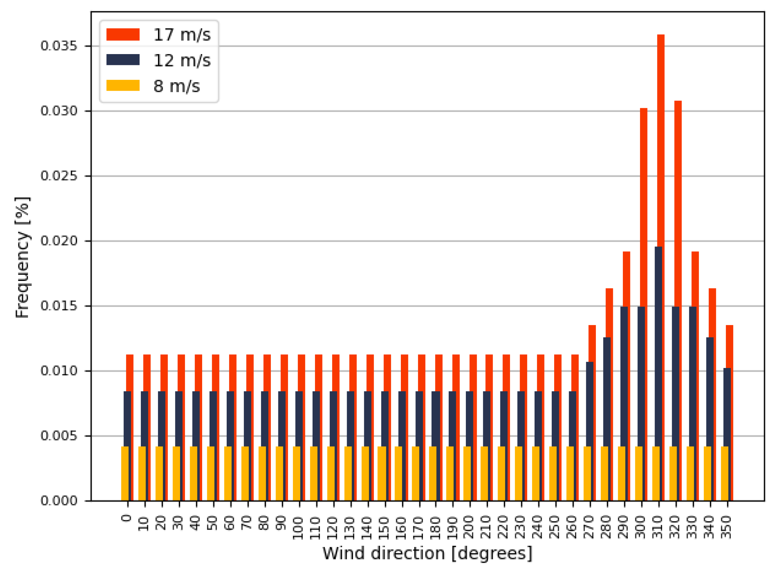
Mosetti et al. [3] proposed three wind scenarios. In the first scenario, the wind speed is constant and equal to 12 m/s. There is only one wind direction from top to bottom (i.e., from North to South). In the second scenario, the wind speed is also constant and equal to 12 m/s, but there are 36 wind directions equally distributed from 0 to 350 degrees in 10-degree increments. In the last wind scenario, there are three wind velocities (8, 12 and 17 m/s) and 36 wind directions. The probability of occurrence is given by Figure 3.

It is valid to state that the power output of the wind turbine, for the first two cases, is a function of the cubed wind velocity given by Equation (8). It follows from the fact that the maximum wind velocity is equal to 12 m/s, which is below the rated speed equal to 12.8 m/s (see Figure 2). This is not the case for the last wind scenario where the maximum wind velocity is equal to 17 m/s. Therefore, we have split the last wind scenario into two subscenarios. In the first, when wind velocity is above 12.8 m/s, the power output remains constant and equal to 630 kW (see Equation (9)), and in the second, the power output is just a function of the cubed wind velocity given by Equation (8).

3. Optimisation Algorithms

In previous works, large numbers of different heuristics and mathematical programming algorithms were applied to the wind farm optimisation problem [34]. The main goal was to minimise the ratio of the two objective functions: wind farm cost and its power output. We applied a single objective hill-climbing algorithm (HCA), described in the following subsection. The two objective functions (cost and power) are optimised directly, without aggregating them, and perform a multi-objective optimisation for which we employed three different evolutionary algorithms. This was done for two main reasons. Firstly, due to the simplicity of the single-objective method, the algorithm is likely to get stuck in local optima, which prevent it from reaching the globally optimal set of solutions. Hence, we need an alternative method to verify HCA performance. Secondly, as there are many publications in which the authors compared the performance of multi-objective algorithms, we decided to do the same for the problem formulated by Mosetti et al.

3.1. Single-Objective Optimisation

Mosetti et al. [3] did not actually propose a single-objective optimisation. Instead, they proposed to apply a weighted sum method to solve this problem. We will discuss this approach in the next subsection. Meanwhile, we will focus on the optimisation proposed by Grady et al. [7] who transformed this problem into a single-objective problem and proposed to minimise the cost (Equation (10)) to power (Equation (9)) ratio:

$$\mathrm{minimise}f=\frac{\mathrm{cost}}{\mathrm{power}}$$

(11)

Both Mosetti et al. [3] and Grady et al. [7] proposed to solve this problem using a genetic algorithm (GA), and according to Azlan et al. [34], around 60% of all authors followed the same path. The remaining authors proposed to apply such approaches as particle swarm algorithms [11], mixed integer programming [12,13], simulated annealing algorithms [14] and Monte Carlo methods [24]. We propose, in this paper, to apply a very simple hill-climbing algorithm (HCA) which is fully described in Algorithms 1 and 2.

Algorithm 1 allows us to find the optimal wind farm layout for a given number of wind turbines. In other words, it maximises the efficiency of the wind farm. In order to find the whole set of solutions, we need to run Algorithm 2. We exploited the fact that there exist only 100 possible locations for wind turbines which implies that the maximum number of wind turbines is also 100. Therefore, by applying Algorithm 2, we were able to find the minimal objective value for each case.

Algorithm 1 Hill-climbing algorithm (HCA) (for fixed number of wind turbines)

1: Define the number of wind turbines, N 2: Randomly place wind turbines on the grid 3: repeat 4:     for $\mathit{wind}\mathit{turbine}=1,2,\dots ,N$ do 5:         Calculate and store farm power output 6:         Identify unoccupied locations on the grid 7:         Move $\mathit{wind}\mathit{turbine}$ to $\mathit{new}\mathit{location}$ 8:         for each $\mathit{new}\mathit{location}$ do 9:            Calculate and store farm power output 10:         end for 11:         Accept farm layout with maximum power output 12:     end for 13: until No better farm power output for N iterations is found

Algorithm 2 Hill-climbing algorithm (HCA) (for all wind turbines (from 1 to 100))

1: for$\mathit{number}\mathit{of}\mathit{wind}\mathit{turbine}\left(s\right)=1,2,\dots ,100$do 2:     Run Algorithm 1 3:     Store position of wind turbine(s) 4:     Store number of wind turbines 5:     Store power output of wind farm 6:     Store cost of the wind farm 7:     Calculate and store the value of the objective function (Equation (11)). 8: end for 9: From the array of the values of objective function identify the one with the lowest value, the corresponding number of wind turbines, cost, power output and wind farm layout.

Unfortunately, even though this procedure is very fast, it has one significant drawback: the HCA can be trapped in a local optimum (minimum in this case). To solve this problem, we apply a different algorithm (e.g., genetic algorithm). By transforming this problem into a multi-objective optimisation problem, we are able to optimise the two objectives directly, representing a better trade-off between the objectives and providing a more effective search of the solution space. The multi-objective algorithms employed in this paper are based on the genetic algorithm, and therefore, they can escape the local minimum.

3.2. Transformation from Single- to Multi-Objective Optimisation

As mentioned in the previous subsection, Mosetti et al. [3] proposed a weighted sum method to solve this problem by minimising the objective function f:

$$\mathrm{minimise}f=\frac{1}{P_{\mathrm{tot}}}{\omega }_1+\frac{{\mathrm{cost}}_{\mathrm{tot}}}{P_{\mathrm{tot}}}{\omega }_2,$$

(12)

where ${\omega }_1$ and ${\omega }_2$ were weights selected by the authors. This formulation is not used herein; thus, we do not report these values. In addition, as stated by the authors, ${\omega }_1$ is small compared to ${\omega }_2$, as more focus was made on finding the lowest cost to power ratio. Unfortunately, this approach poses significant problems. It is very difficult to set the weights’ values (the authors did not report these values), all objectives need to be converted into one type (minimisation or maximisation) and, finally, a large number of tests are needed to determine if the optimal solution set is found [18]. 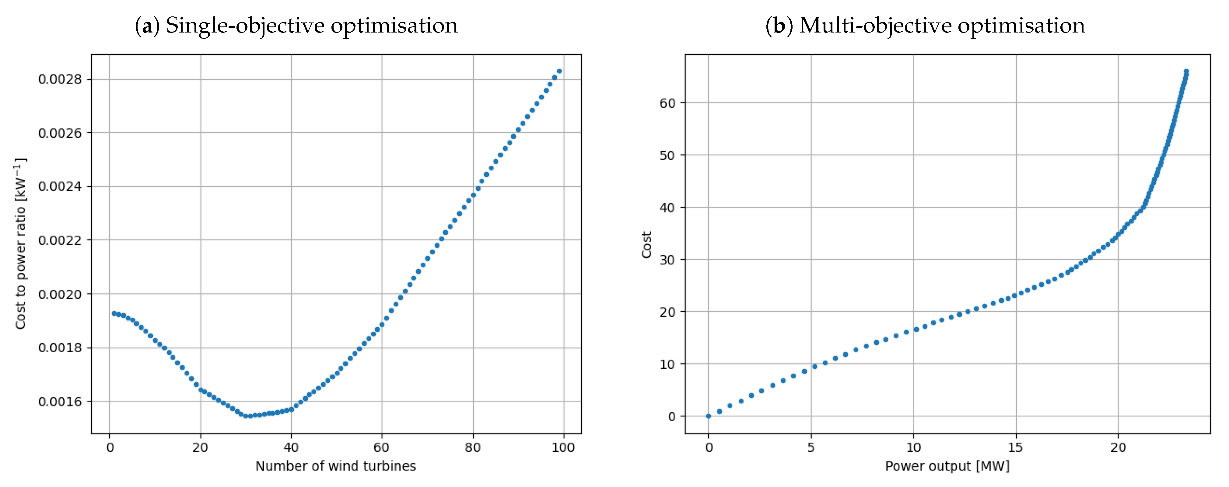While it is possible to identify good parameters for the objective weights ${\omega }_1$ and ${\omega }_2$—for example, by using sensitivity analysis—we note that this would not improve the search procedure, as it would still involve using an aggregated single-objective problem formulation, which would need multiple runs to identify an approximation to the true Pareto front. 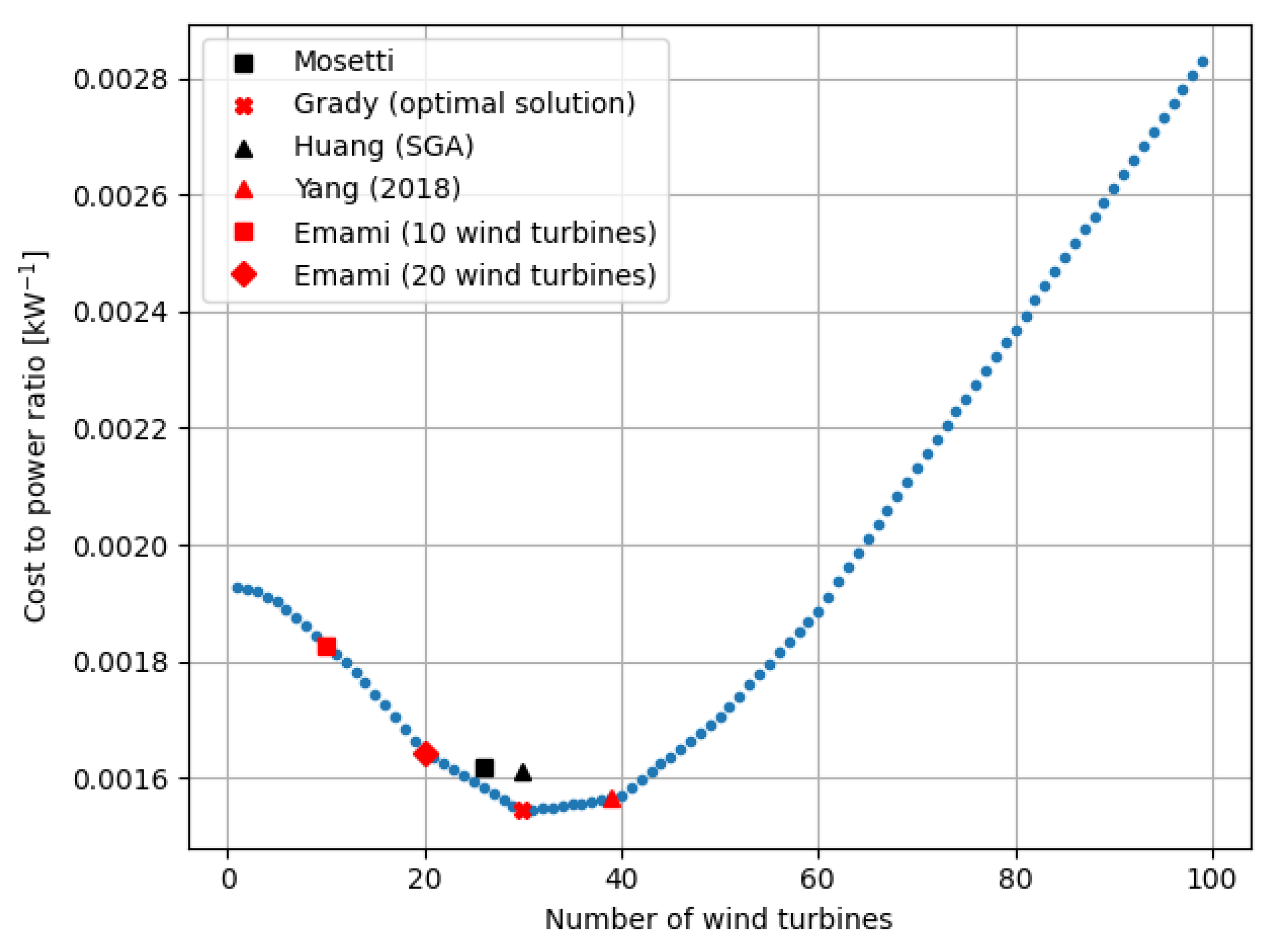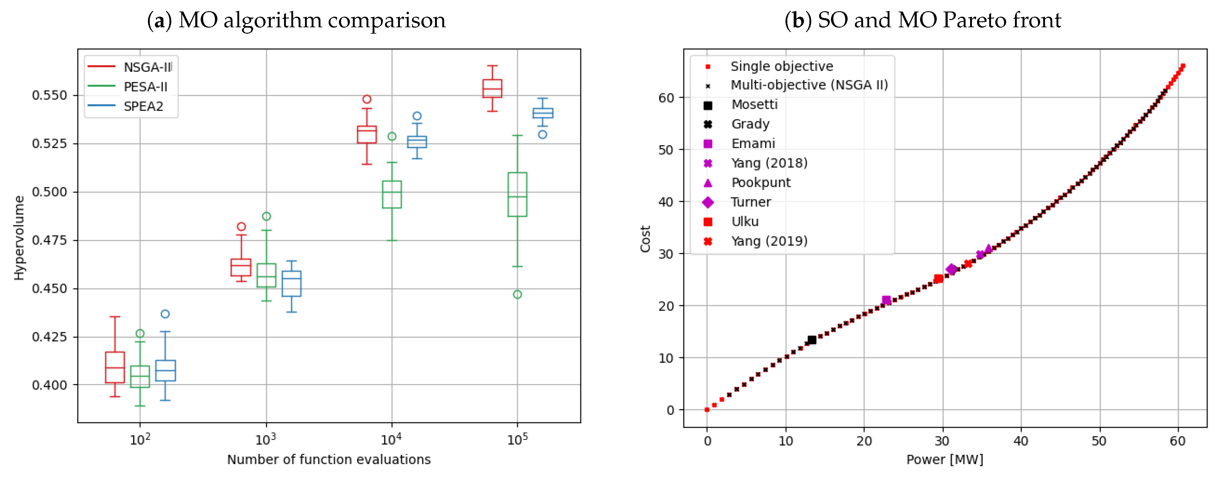To solve this problem, we can simply transform it from single- to multi-objective optimisation as shown in Figure 4. Using a multi-objective algorithm to identify the Pareto front approximation in a single search process enables a more efficient exploration of the search space. The two subfigures show two different views of the same set of solutions.

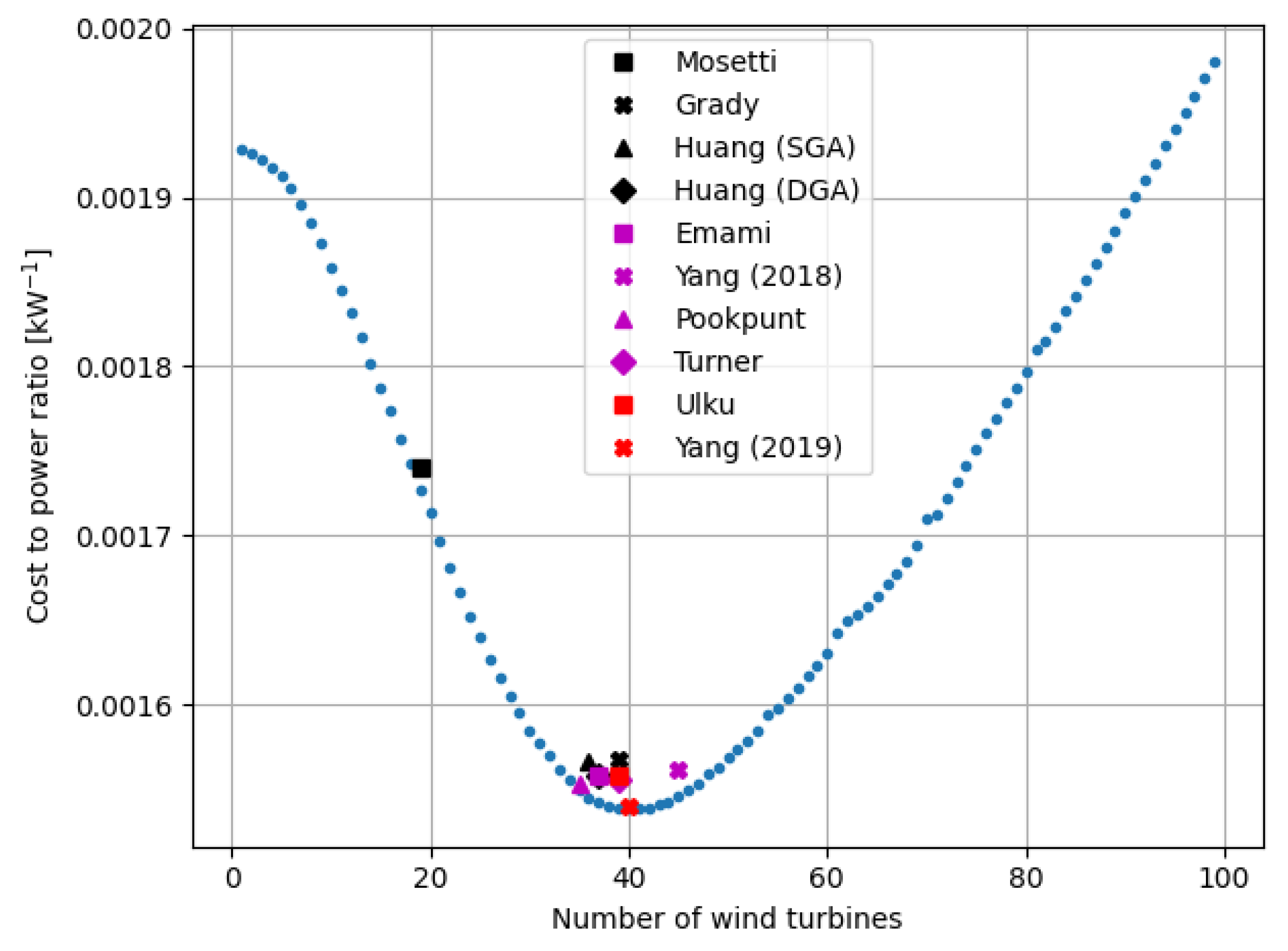
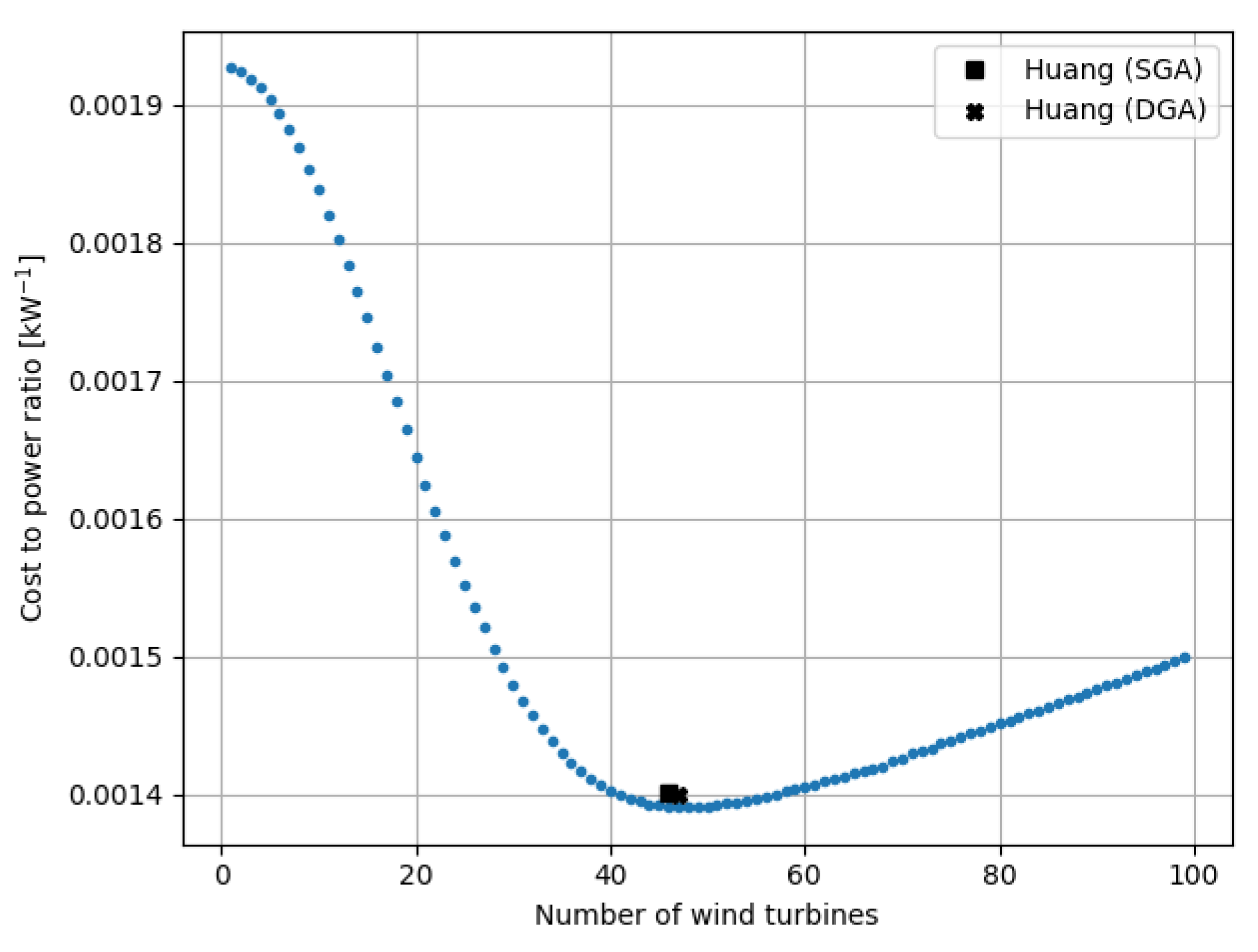
Figure 4a shows the results from the single-objective optimisation. Each blue dot represents the ratio (cost to power) for a given number of wind turbines. We can easily determine that the optimal solution (minimum ratio) exists for 30 wind turbines (this is an actual solution for case 1 which we will discuss in the next section). In Figure 4b, the same set of solutions is a represented in a different way. We overlook the objective function and instead determine the trade-off between the cost and the ratio.

3.3. Multi-Objective Optimisation

In this subsection we will briefly introduce the concept of multi-objective optimisation. We will introduce the Pareto front, non-dominance, three evolutionary algorithms (EAs) and the hypervolume indicator.

3.3.1. Introduction to Multi-Objective Optimisation

In general, in single-objective optimisation, we are looking for one solution only (in this paper, to transform the wind farm layout problem from single- to multi-objective, we found an optimal solution for each number of wind turbines). In multi-objective optimisation, the number of optimal solutions could be infinite and form a Pareto front. In this paper we have two conflicting objectives: we wish to minimise the cost of the wind farm and, at the same time, maximise the power output. Both objectives cannot be achieved at the same time, and hence there must be a trade-off between the cost and the power (Figure 4b). To illustrate this, let us consider Figure 5.

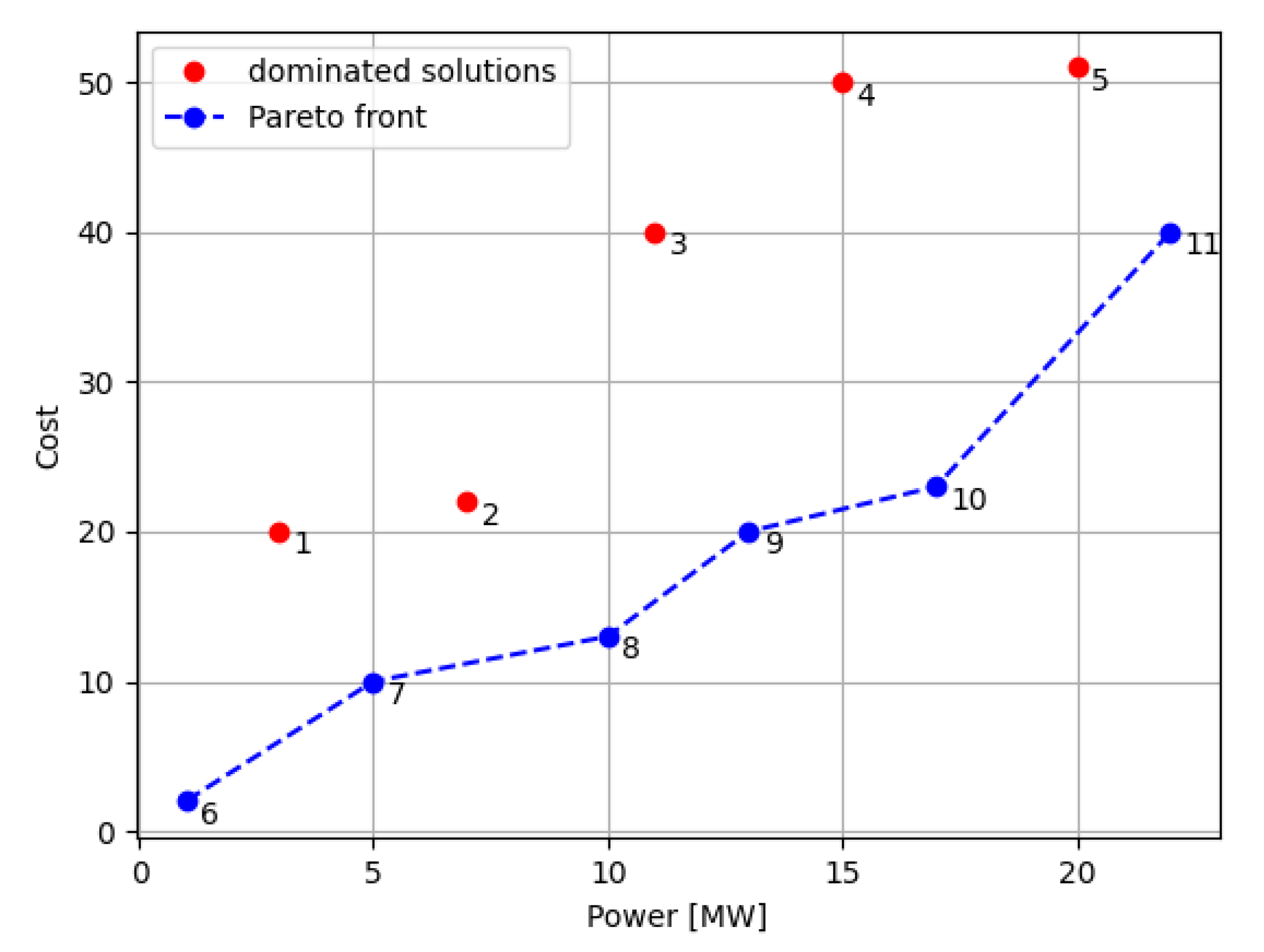
In Figure 5, solutions are plotted and are denoted by red and blue dots. The blue dots form a Pareto front of optimal solutions because they dominate the red dots. To understand the concept of dominance, let us observe solution 7. Solution 7 has a higher power output and smaller cost than solution 1. Therefore, we claim that solution 7 dominates solution 1. On the other hand, solution 2 is not dominated by solution 7 because solution 2 has a higher power output than solution 7. However, solution 2 is dominated by solution 8 (and 9) because solution 8 has a higher power output and lower cost. Furthermore, when we consider solutions 6 and 7, we notice the following: solution 6 has a smaller power output, but it also has a smaller cost. Therefore, we claim that solutions 6 and 7 are nondominated solutions. Finally, we can claim that solutions 6–11 dominate solutions 1–5 and thus form a Pareto front of the nondominated solutions. Solutions in the Pareto front are mutually nondominating, such that for any pair of Pareto optimal solutions, neither dominates the other.

The formal definition of dominance in the multi-objective optimisation problem is as follows. Consider two solutions x and y. We say that solution x dominates y if solution x is no worse than solution y in all objectives and solution x is strictly better than y in at least one objective [18].

Since we have introduced the basic idea of multi-objective optimisation, we are now ready to discuss the multi-objective algorithms that were applied in this paper.

3.3.2. Evolutionary Algorithms

Multi-objective evolutionary algorithms are employed to solve problems that cannot be easily solved and when there are at least two conflicting objective functions that need to be maximised (i.e., power) and/or minimised (i.e., cost) at the same time. This can be accomplished by implementing the genetic algorithm, which is a workhorse of the algorithms that we evaluated in this paper. Such algorithms maintain a population of solutions, and at each generation, solutions are found by the recombination (crossover) of the existing or initial randomly generated solutions. In order to maintain the diversity in solutions, a small number of solutions are perturbed with a mutation operation. Finally, the solutions are sorted with respect to spread and dominance. In this paper, three multi-objective evolutionary algorithms were applied: nondominated sorting genetic algorithm II (NSGA-II) [18], strength Pareto evolutionary algorithm 2 (SPEA2) [17] and region-based Pareto envelope-based selection algorithm (PESA-II) [19].

In NSGA-II, the initial randomly generated population is sorted with respect to nondominance and crowding distance. Offspring are then generated using the standard binary tournament selection, recombination and mutation operators. The fitness value for each solution (parent and offspring) is then assigned based on nondominance and crowding distance and sorted. This way, elitism is used to drive the search population toward the Pareto front. From the whole population (both parents and offspring), half of the worst solutions are disregarded, and the whole process repeats until the stopping criterion is reached (e.g., computation time, number of function evaluations) [18].

SPEA2 is also an elitist multi-objective evolutionary algorithm which means that the fitness value is assigned to each solution, all of which are sorted in ascending order. To calculate the fitness value of the solution i, we need to know how many other solutions are dominating solution i, how many solutions are dominated by solution i and the distance of solution i with respect to other solutions (this preserves the diversity of solutions). Then, the best solutions are stored in the archive. We repeat the whole process for a fixed budget of function evaluations [17].

The authors of PESA-II claim that their algorithm ‘outperform[s] earlier approaches on various problems’ [19]. The major difference between the discussed algorithms and PESA-II is a fitness values assignment. In NSGA-II and SPEA2, the fitness value is assigned to the individual solution. In PESA-II, the fitness value is assigned to the hyperbox in objective space that is occupied by at least one solution. This approach claims to guarantee convergence to the true Pareto front in a smaller number of function evaluations and a better spread of solutions in the approximated Pareto front [19]. The multi-objective algorithm parameters used are given in

Table 2. Parameters for multi-objective algorithms (‘nv’ denoting the number of variables).

Parameters	NSGA-II	SPEA2	PESA-II
Population size	100	100	100
Polynomial mutation distribution index	15	15	15
SBX distribution index	20	20	20
Mutation probability	1/nv	1/nv	1/nv
Size of external archive	N/A	100	100

.

At this point, it is necessary to introduce the metric that we will use to measure the performance of multi-objective evolutionary algorithms. An ideal metric should measure two goals simultaneously: convergence (i.e., how close the solutions are to the Pareto front) and diversity (i.e., how well solutions are spread). Therefore, we can split metrics into three groups: metrics that measure convergence (e.g., error ratio, set coverage metric, generational distance), metrics that measure diversity (e.g., spacing, spread, maximum spread, chi-square-like deviation measure) and types of metrics that measure both convergence and diversity at the same time (e.g., hypervolume, weighted metric) [18]. We decided to use hypervolume metrics which we will discuss next.

3.3.3. Hypervolume Indicator

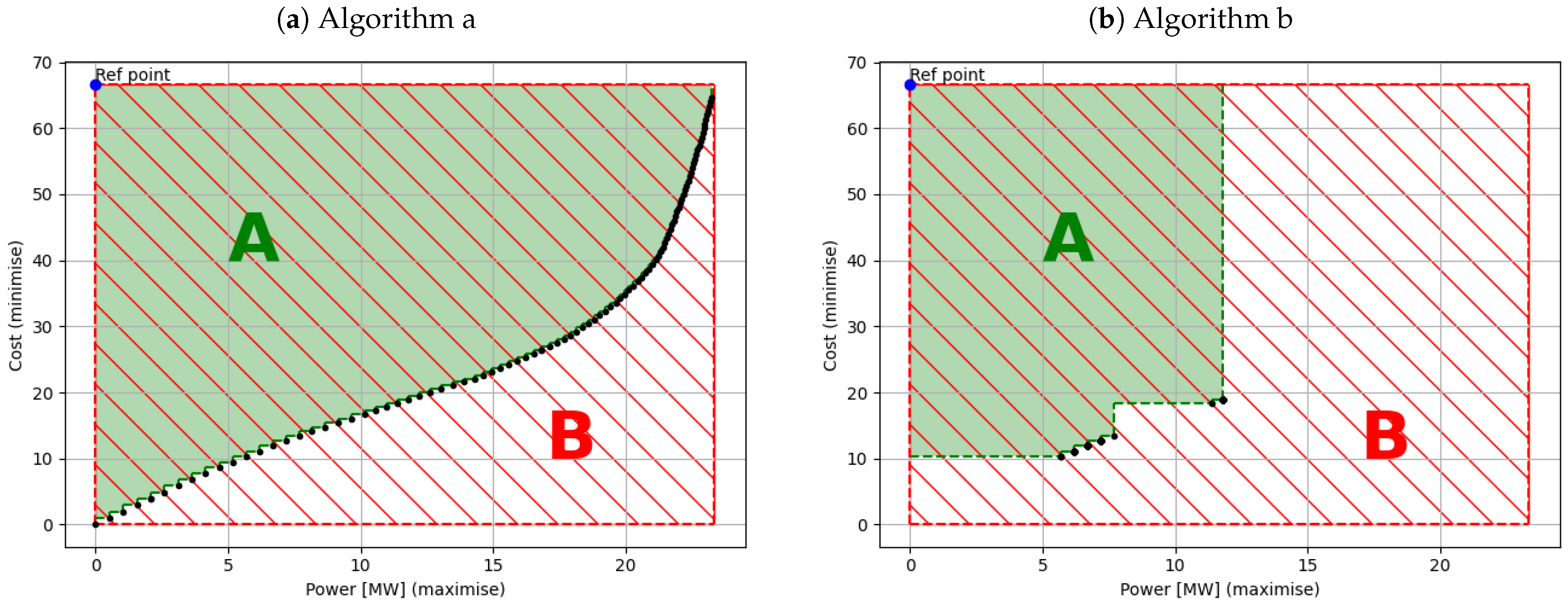
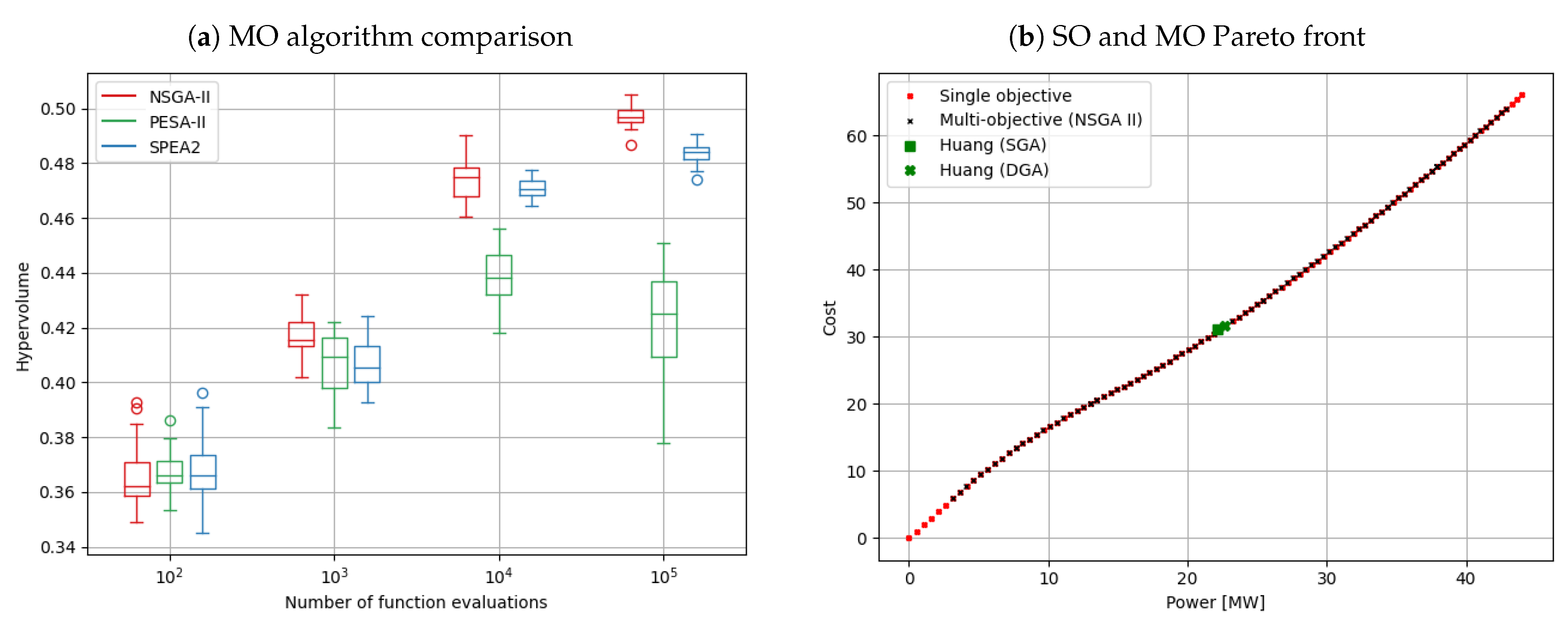
The hypervolume indicator is one of the metrics that measure the performance of multi-objective evolutionary algorithms. It should only be applied if the magnitude of the two objectives is the same. To illustrate how it works, we evaluated two different algorithms for the same number of function evaluations and plotted the solutions denoted by the black dots in Figure 6.

In the aforementioned figure, the search space is represented by the area B. For this problem, it was possible to determine the search space because the minimum and the maximum values of the objective functions (cost and power of the wind farm) were known in advance. The minimum cost and power occurs when the number of wind turbines is zero (i.e., not a practical solution). Additionally, due to a discrete number of wind turbines, we know that the maximum cost and power will occur when the number of wind turbines is equal to 100. The maximum cost will be the same for all wind scenarios, as the cost depends on the number of wind turbines. On the other hand, the maximum power output will depend on the wind velocity and the wake effect, and hence it will be different for every wind scenario. In order to find the hypervolume value (area A), we need to know the coordinates of the reference point. The reference point is the vector containing the worst objective value in the population for each objective, e.g., in this case, the worst value for objective 1 (maximum cost) and the worst value for objective 2 (minimum power), as shown on each subfigure. We then need to connect the points (solutions) as shown by the dashed green line and calculate the hypervolume (area A). Finally, in order to normalise the result, we need to divide area A by area B.

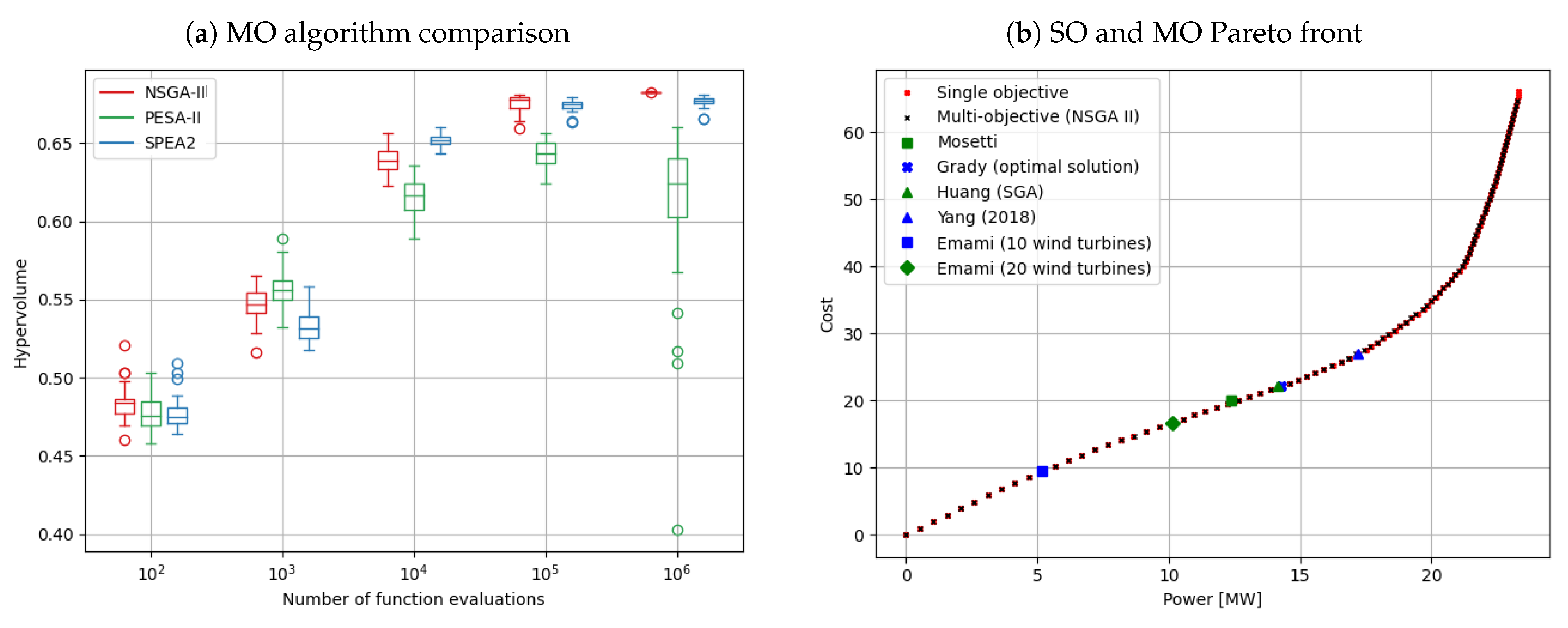
From Figure 6a, we can clearly see that Algorithm (a) performed very well. The solutions are fairly equally spaced and are well spread over the search space. On the other hand, Algorithm (b) did not perform that well. The Pareto front approximation contains only a few solutions, and the spread is rather poor. In this paper, we only deal with two objective functions, and therefore it is easy to visualise the results. Nevertheless, the normalised hypervolume indicators for Algorithm (a) and Algorithm (b) are equal to 0.682894 and 0.402976, respectively, which reflects their performance well.

Until now, we have provided the reader with a description of the wind farm modelling and an introduction to single- and multi-objective optimisation. In the next section, which is the heart of this paper, we present and discuss our findings.

4. Case Study

In this section, we will discuss the results for four different wind scenarios, which we briefly described in Section 2.7. In each scenario, we ran the single-objective HCA optimisation algorithm and the three multi-objective optimisation algorithms (NSGA-II, SPEA2 and PESA-II). The multi-objective optimisation algorithms were executed 30 times for each given number of function evaluations to ensure the sample size was sufficient for statistical analysis. We started with 100 function evaluations for each algorithm and then increased by a factor of 10 until 100,000 function evaluations were reached for cases 3 and 4, and 1,000,000 function evaluations for cases 1 and 2. The number of function evaluations was not identical since the computational time for cases 1 and 2 was much shorter than for that of cases 3 and 4.

4.1. Case 1

4.1.1. Single-Objective Optimisation

In the simplest case, a constant 12 m/s wind speed and top to bottom wind direction was adopted. Figure 7 is a representation of the optimal wind farm layouts found by various authors. Each dot on the grid represents the position of the wind turbine. The optimal wind farm layout for 30 wind turbines (Figure 7a), and consequently the optimal value of the objective function (Equation (11)), was found by most of the researchers (

Table 3. Results comparison for case 1.

		Reported			Calculated
Author(s)	N	Power [kW]	Obj. Value	Eff. [%]	Power [kW]	Obj. Value	Eff. [%]
Mosetti et al., 1994 [3]	26	12,375.00	0.0025700	95.00	13,478.34	0.0016195	91.65
Grady et al., 2005 [7]	30	14,310.00	0.0015436	92.02	14,304.22	0.0015442	91.98
Huang et al., 2007 [8] (SGA)	30	13,940.57	-	89.64	14,149.20	0.0015611	90.98
Huang et al., 2007 [8] (DGA)	30	14,118.60	-	90.78	14,304.22	0.0015442	91.98
Emami et al., 2010 [9] (a)	10	5184.00	-	100.00	5183.99	0.0018263	100.00
Emami et al., 2010 [9] (b)	20	10,164.00	-	98.00	10,139.85	0.0016423	97.80
Emami et al., 2010 [9] (c)	30	14,310.00	-	92.00	14,304.22	0.0015442	91.98
Pookpunt et al., 2013 [11]	30	14,310.00	0.0015440	92.01	14,304.22	0.0015442	91.98
Turner et al., 2014 [12]	30	14,800.00	0.0012739	-	14,304.22	0.0015442	91.98
Yang et al, 2018 [10]	39	17,768.00	0.0015150	-	17,188.87	0.0015662	85.02
Ulku et al., 2019 [13]	30	16,148.71	0.0014000	-	14,304.22	0.0015442	91.98
Yang et al., 2019 [14]	30	14,269.00	0.0015479	91.76	14,304.22	0.0015442	91.98
Present (SO and MO)	30	-	-	-	14,304.22	0.0015442	91.98

—optimal value shown in bold).

Grady et al. [7], under identical conditions proposed by Mosetti et al. [3], stated that the calculation for each column can be done independently, as the wake effect from the neighbouring columns does not occur. It can be shown using Equation (5), as well as intuitively, that this assumption is incorrect. The first set of authors reported that for a single column, the power output is 1431 kW. This result was later extrapolated to the remaining columns, and the declared power output of the wind farm was equal to 14,310 kW. In our model, the power output of the wind farm is equal to 14,304 kW, as we implemented the partial wake effect. This is a small difference, albeit significant.

All the results from the considered papers were gathered in Table 3. Even though most authors found (what we believe to be) an optimal solution for 30 wind turbines, the reported power output is not equal to 14,310 kW (or 14,304 kW). The lack of alignment between the results is disconcerting, as it indicates that there could be differences in implementation of the Jensen wake model. Furthermore, Yang et al. [10] reported that the optimal solution exists for 39 wind turbines (Figure 7d and Table 3) with the corresponding objective value smaller than that of the solution provided by this paper (and past papers as well). After implementing the Yang et al. [10] optimal wind farm layout in our model, we calculated that the corresponding objective value is larger than that presented in this paper (Table 3). Emami et al. [9] reported the optimal solutions for 10, 20 (Figure 7c) and 30 wind turbines. The authors’ objective function for case 1 was defined differently than ours, giving this difference. Nevertheless, Emami’s and Yang’s solutions are indeed optimal for the given number of wind turbines shown in Figure 8.

4.1.2. Multi-Objective Optimisation

The results for this case using the multi-objective optimisation algorithms introduced earlier were plotted in Figure 9a. Each boxplot represents the distribution of the data collected for each algorithm across the given number of function evaluations. We can see that the hypervolumes for 100- and 1000-function evaluations were very similar for all three algorithms. As the number of function evaluations increases, the highest hypervolume was obtained for NSGA-II. Furthermore, the standard deviation for one million function evaluations for NSGA-II is very low compared to other algorithms, and therefore, we conclude that the NSGA-II performed the best. We then plotted the nondominated solutions (the Pareto front approximation)—this is shown in Figure 9b. Additionally, in order to make a comparison with the results found using the single objective algorithm (HCA), we split the single-objective function into cost and power functions and put them on the same graph (Figure 9b). It can be clearly seen that these solutions overlap, and hence we deduce that the single- and multi-objective (MO) approach returned the same results.

We also noted that the range of results for one million function evaluations from the PESA-II algorithm is large, and in general, the hypervolume is lower than that of the two other algorithms. Hence, we claim that for this particular problem, PESA-II did not perform very well. This may be due to the fact that the PESA-II algorithm fitness value is assigned to the hyperboxes, contrary to NSGA-II and SPEA2 where the fitness value is assigned to the individual solution. The set of solutions for PESA-II for one million function evaluations with the corresponding hypervolume equal to around 0.4 was presented in Figure 6b.

4.2. Case 2

4.2.1. Single-Objective Optimisation

The wind speed for this case is also constant and equal to 12 m/s. In contrast to case 1, there are 36 wind directions, equally spaced from 0 to 350 degrees with 10-degree increments. Due to the number of wind directions, an intuitive solution is difficult to find, but it can be deduced that the highest power output occurs from wind turbines located on the edges of the wind farm.

Contrary to case 1, no optimal solution was found, with no two authors declaring the same solution to be the optimal one (Figure 10 and

Table 4. Result comparison for case 2.

		Reported			Calculated
Author(s)	N	Power [kW]	Obj. Value	Eff. [%]	Power [kW]	Obj. Value	Eff. [%]
Mosetti et al., 1994 [3]	19	8711.00	0.0018400	88.00	9221.97	0.0017399	93.63
Grady et al., 2005 [7]	39	17,220.00	0.0015666	85.17	17,171.76	0.0015678	84.93
Huang et al., 2007 [8] (SGA)	36	14,705.94	-	78.80	16,125.59	0.0015664	86.41
Huang et al., 2007 [8] (DGA)	37	15,040.28	-	78.41	16,566.26	0.0015577	86.37
Emami et al., 2010 [9]	37	17,335.00	-	90.40	16,567.67	0.0015576	86.38
Pookpunt et al., 2013 [11]	35	-	-	-	15,919.72	0.0015526	87.74
Turner et al., 2014 [12]	39	18,336.00	-	-	17,309.69	0.0015553	85.62
Yang et al, 2018 [10]	45	20,347.00	0.0014946	-	19,501.36	0.0015610	83.60
Ulku et al., 2019 [13]	36	16,483.88	0.0015000	-	16,217.02	0.0015575	86.90
Yang et al., 2019 [14]	40	14,269.00	0.0015479	91.76	17,847.58	0.0015403	86.07
Present (SO)	41	-	-	-	18,246.48	0.0015382	85.85
Present (MO)	41	-	-	-	18,246.48	0.0015382	85.85

). Furthermore, the number of wind turbines reported also varies. The general conclusion is that there should be around 40 wind turbines, and they should be positioned on the edges of a wind farm. Intuitively, as there is only one wind speed and there are equally spaced wind directions, the wind farm layout should be somehow symmetric. This is true for this paper (Figure 10a) and the layouts reported by Pookpunt et al. (Figure 10i), Ulku et al. (Figure 10j) and Yang et al. (Figure 10j). From Figure 10, we can deduce that the optimal solution was reported in the current paper and by Yang et al. [14]. The results gathered in Table 4 confirm this observation: the reported objective values and the efficiencies of the wind farm are very similar.

This case has two interesting wind farm layouts, those reported by Huang et al. [8] (Figure 10g) and Emami et al. [9] (Figure 10f). The layouts are very different, but the number of wind turbines, the farm efficiency and the objective value are almost identical. This leads to the conclusion that there may exist a large set of optimal or sub-optimal solutions, giving a lot of flexibility for wind farm design.

4.2.2. Multi-Objective Optimisation

The multi-objective results for case 2 (Figure 12a) are almost identical with the results obtained for case 1. As before, for one million function evaluations, the highest hypervolume and the minimum standard deviation were found for NSGA-II. In addition, the reported Pareto front overlaps with the solutions reported for a single-objective optimisation algorithm (Figure 12b). The optimal layout for 41 wind turbines using NSGA-II was slightly different (Figure 10b) than the one found using the single-objective approach (Figure 10a). However, this is strictly due to symmetry, meaning that we may deduce that there exist two other optimal wind farm layouts with the same number of wind turbines, wind farm efficiency and fitness function. It can also be noted that the solutions plotted in Figure 11 from the multi-objective optimisation point of view are equally good, as they lie on the Pareto front (Figure 12b).

4.3. Case 3

In case 3, there are 36 equally spaced wind directions with varied initial wind speeds (8, 12 and 17 m/s), as shown in Figure 3. The main difficulty with case 3 is best reflected in Figure 13. The red dotted line represents the wind turbine power curve where the rated speed was not taken into consideration. In other words, the power generated by the wind farm is only dependent on the wind speed (Equation (8)). This is not consistent with the wind farm modelling proposed by Mosetti et al. (Figure 2 and Figure 13). It appears that, among the considered papers, one author adopted the proposed model. The reason why this was not significant for previous cases is the fact that the maximum wind velocity was below 12.8 m/s (cut-out speed). In this case, the maximum wind velocity is equal to 17 m/s for which the power output is equal to 1474 kW, above the rated power output of 630 kW. Therefore, we split this case into case 3 (the Mosetti et al. model) and case 4 (not).

4.3.1. Single-Objective Optimisation

The only paper we could compare our results with, in this particular case, was that of Huang et al. [8]. The reader may be surprised to learn that the result of Mosetti et al. does not seem to be taken into account here. When we discuss case 4, it will become clear why it was done in this manner. The optimal number of wind turbines reported by Huang et al. was 47 (Figure 14d), and most, although not all, wind turbines were located on the edges of the wind farm. Our findings were similar, i.e., the edges of the wind farm were completely occupied by wind turbines, and the remaining wind turbines formed a symmetric shape in the middle of the wind farm (Figure 14a). Our objective value was lower than the one reported by Huang et al. (

Table 5. Result comparison for case 3.

		Reported			Calculated
Author(s)	N	Power [kW]	Obj. Value	Eff. [%]	Power [kW]	Obj. Value	Eff. [%]
Huang et al., 2007 [8] (SGA)	46	20,087.80	-	84.26	22,174.57	0.0014004	92.93
Huang et al., 2007 [8] (DGA)	47	20,430.70	-	83.87	22,631.96	0.0013993	92.83
Present (SO)	48	-	-	-	23,226.49	0.0013902	93.28
Present (MO)	48	-	-	-	23,215.73	0.0013909	93.24

), indicating that the HCA returned better results than their genetic algorithm.

The attentive reader has already noticed that the optimum number of wind turbines increases with each case. For cases 1, 2 and 3, the optimal number of wind turbines was 30, 41 and 48, respectively. This is due to the fact that in case 1, only 10 wind turbines in the top row were upstream wind turbines, and in case 2, around 20 wind turbines were located on the edges, mostly not encountering the wake effect (hence exhibiting higher power output). Finally, for case 3, the dominating wind velocity was equal to 17 m/s. Since the wake effect can be accountable for up to 30% loss [2] in wind speed, the wind speed can decrease from 17 m/s to around 12 m/s, which is very close to the rated power output of the wind turbine (630 kW). In other words, we can have more wind turbines on the grid with higher (or similar) wind farm power output and efficiency. For example, the efficiency for case 1 (30 wind turbines) was equal to 92%, for case 2 (41 wind turbines) 86% and for case 3 (48 wind turbines) 93%.

4.3.2. Multi-Objective Optimisation

As previously stated, due to the computational expense, we were restricted to running 100,000 function evaluations for cases 3 and 4 instead of the one million function evaluations performed for cases 1 and 2. From Figure 16a, we can clearly see that NSGA-II outperformed two other algorithms (for 100,000 function evaluations). The Pareto front approximation overlaps the solutions generated using the HCA as shown in Figure 16b. The spread of solutions is not as good as for the two previous cases due to the smaller number of function evaluations. Moreover, the optimal layout for 48 wind turbines (Figure 14b) is similar to the optimal layout found using the HCA (Figure 14a), and the values of objective functions (Table 5) are almost identical. Furthermore, as we look at Figure 16b, the solutions presented by Huang et al. can also be considered equally as good (Figure 15 and Figure 16b).

4.4. Case 4

4.4.1. Single-Objective Optimisation

To understand the results for case 4, we need to remind ourselves of case 2. In both cases, there were 36 wind directions. However, in case 2, there was only one wind speed (12 m/s), and in case 4, the wind speed varied (8, 12 and 17 m/s). Intuitively, we could say that the results will be completely different. This is true when it comes to the optimal objective values: 0.0015382 for case 2 (Table 4) and 0.0008430 for case 4 (

Table 6. Result comparison for case 4.

		Reported			Calculated
Author(s)	N	Power [kW]	Obj. Value	Eff. [%]	Power [kW]	Obj. Value	Eff. [%]
Mosetti et al., 1994 [3]	15	3695.00	0.0036100	84.00	13,311.15	0.0010052	94.60
Grady et al., 2005 [7]	39	32,038.00	0.0008031	86.62	31,238.40	0.0008618	85.39
Emami et al., 2010 [9]	28	32,261.63	-	91.00	22,825.17	0.0009223	86.90
Pookpunt et al., 2013 [11]	46	39,359.00	0.0007894	89.83	35,883.91	0.0008654	83.16
Turner et al., 2014 [12]	39	32,453.00	-	-	31,130.04	0.0008648	85.09
Yang et al, 2018 [10]	45	20,347.00	0.0014946	-	19,501.36	0.0015610	83.60
Ulku et al., 2019 [13]	36		0.0010000	-	29,471.85	0.0008570	87.27
Yang et al., 2019 [14]	41	33,966.00	0.0008263	88.31	33,261.02	0.0008438	86.48
Present (SO)	41	-	-	-	32,608.54	0.0008430	86.90
Present (MO)	41	-	-	-	32,605.88	0.0008431	86.90

). However, in terms of the number of wind turbines, the wind farm layouts and the efficiency of the wind farm, the results are very similar (this was noted earlier by Yang et al. [14]). The relative positions of the optimal solutions for a given number of wind turbines are almost identical (Figure 17). We found the optimal number of solutions to be identically equal to 41 (Table 4 for case 2 and Table 6 for case 4). Finally, in the optimal wind farm layout for case 4, most wind turbines are on the edges of the farm (Figure 18a), similar to case 2 (Figure 10a).

As stated above, the optimal objective values found by Yang et al. [14] were very similar to ours. Other authors, Pookpunt et al. and Mosetti et al., also found optimal solutions for a given number of wind turbines as shown in Figure 17b. The reason why we decided to include the findings of Mosetti et al. is because all previous authors who included the Mosetti et al. wind farm layouts in their papers recalculated the power output and the efficiency of the wind farm using the initial settings for case 3. That is, they ignored the rated power factor. Hence, we decided to include the findings of Mosetti et al. in this section.

4.4.2. Multi-Objective Optimisation

It comes as no surprise that the best performing algorithm for 100,000 function evaluations was again NSGA-II (Figure 19a). The Pareto front approximation overlaps the solutions found using the single-objective algorithm (Figure 19b). The optimal wind farm layout for 41 wind turbines (Figure 18a) is very similar to the layout found using the HCA (Figure 18b). The solutions reported by other authors (Figure 19b) lie very close to the Pareto front approximation, and from the decision maker’s point of view, they can also be considered as optimal.

5. Conclusions

According to Yang et al. [14], “…the cost model and the objective function, which were suggested by Mosetti et al. to obtain the optimal layout, have a trade-off between efficiency and cost, and this problem should be addressed in future works.” We could not agree more.

In this paper, we performed a single- and multi-objective optimisation to the problem that was proposed by Mosetti et al. In the single-objective optimisation, we adopted a hill-climbing algorithm (HCA), showing that it can provide better results than more sophisticated algorithms. This leads to an interesting conclusion that it may not be worth drawing your sword to kill a fly as the problem complexity should be well aligned with the chosen method. Our approach was fast and simple, and, because of this, we not only found the optimal solution for each case but also provided the reader with a whole set of solutions for a given number of wind turbines. As a consequence, we could then turn this into a multi-objective optimisation problem.

The main disadvantage of the HCA was the procedure that had to be adopted to find the whole set of solutions, i.e., we needed to run the HCA for each number of wind turbines and calculate the value of the objective function. This was not the case when we performed the multi-objective optimisation. We were able to find the whole set of solutions in a single attempt. Furthermore, in the single-objective optimisation we exploited the discrete layout of the wind farm. Applying HCA would not be possible if the wind farm layout was continuous. In other words, the multi-objective optimisation is a truer representation of the actual problem.

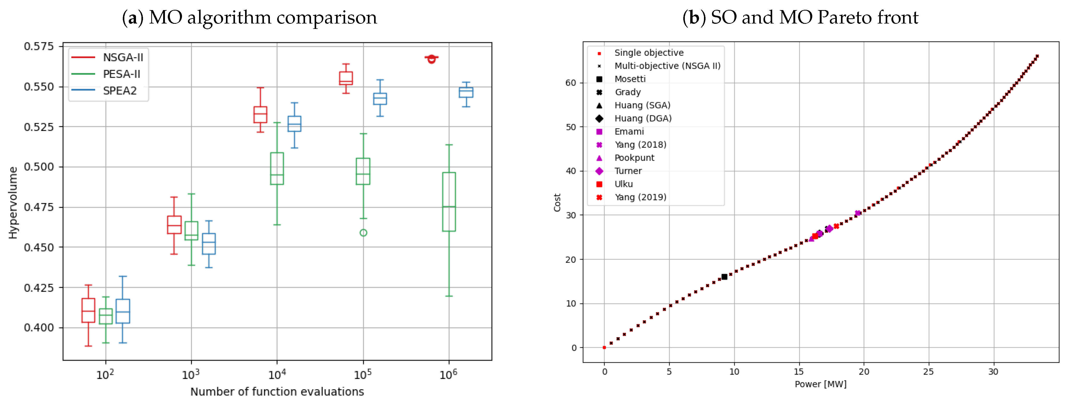
In the multi-objective part of the paper, we explained the concept of evolutionary algorithms and successfully applied three algorithms: NSGA-II, SPEA2 and PESA-II. We showed that the best performing algorithm for each case was NSGA-II. Because the transformation from single- to multi-objective optimisation was possible, we were able to compare the results of NSGA-II and HCA and noted that the results were almost identical. Finally, we have compared our findings with past papers and demonstrated that solutions disregarded by some authors could be considered optimal from the decision maker’s point of view. In other words, this gives us a lot of flexibility when it comes to wind farm design. We have also shown that for this particular problem, the PESA-II algorithm did not perform well.

Future work may focus on other wind turbine technologies and on distinct grid representations (e.g., continuous grids [5]). The transformation from a discrete to continuous wind farm layout should be made and would release the full potential of multi-objective evolutionary algorithms.