Robust Parameter Estimation of an Empirical Manoeuvring Model Using Free-Running Model Tests

Abstract

The work presents the identification and validation of the hydrodynamic coefficients for the surge, sway, and yaw motion. This is performed in two ways: using simulated data and free-running test data. The identification and validation with the simulation data are carried out using a 25° turning test and a 20°−20° zigzag manoeuvring test. For the free-running test data, two zigzag manoeuvres are used: 30°−30° zigzag for identification and 20°−20° zigzag for validation. A nonlinear manoeuvring model is proposed based on the standard Euler equations, and the hydrodynamic coefficients are computed using empirical equations. To obtain robust results, the truncated singular value decomposition is employed to diminish the multicollinearity and the parameter uncertainties due to noise. The validation is carried out by comparing the result of the measured values with the predictions obtained using the manoeuvring models. Finally, a sensitivity analysis for the simulation data is performed to understand the influence of the parameters in the manoeuvres.

1. Introduction

Ship manoeuvrability is an important topic in the shipbuilding and shipping industries, and it was traditionally evaluated by carrying out massive captive ship model tests. Mathematical manoeuvring models are essential to the study of manoeuvrability [1]. System identification (SI) is a mature technology to fit the mathematical models of dynamical systems to measured data. It was only introduced for ship motion modelling in the 1960s, and it became more developed recently [2,3,4,5,6,7,8]. It is also possible to develop methods based on artificial intelligence techniques [9,10], but they do not include explicit information on the physics of the process and thus the methods that identify the parameters of mathematical models are often preferred as these models can easily be used to simulate the ship trajectories [11,12].

When studying ship manoeuvrability, physical tests are fundamental. These can be full-scale tests [13,14], which are the most accurate, but they are expensive. Ship model tests, such as captive tests [15,16] or free-running tests [17], are another, cheaper option. Captive tests can be more expensive [18,19,20,21,22] than free-running tests. Model tests face scale effect problems which can be avoided with system identification methods [1,22]. The most plausible and direct manner to confirm ship manoeuvring properties is often free-running tests.

The focus of this paper is the computation of the hydrodynamic coefficients for a nonlinear manoeuvring mathematical model. When computing several coefficients at the same time, the model’s accuracy can be compromised due to the multicollinearity [19,20,21,23], dynamic cancellation effects [18,24], parameter drift [18], and noise contained in the data. They are the main issues faced when trying to obtain robust parameters. They are all linked together and consequently compromise the robustness of the estimation and therefore the obtained parameters are sensitive to noise. To achieve robust results, extensive experimental data should be used, tests should be combined with system identification methods not computing too many coefficients at the same time [1,24,25], and the parameter uncertainty due to noise should be carried out.

The number of mathematical manoeuvring models is very extensive [1,20]. The Abkowitz model, the Nomoto model, and the MMG model are the most used in manoeuvrability studies [26]. Manoeuvring models are often complex, gathering a set of motion equations, mainly surge, sway, and yaw. The hydrodynamic forces and moments are expanded to their Taylor expansion, where the hydrodynamic coefficients can be found [25].

Several SI methods, such as the extended Kalman filter [27], global optimization algorithm, truncated least squares support vector machine [19,20,21,28,29], genetic algorithm [22,23,24,25,26,27,28,29,30], particle swarm optimization [31], and artificial neural network [32] can be used to estimate hydrodynamic coefficients.

Sutulo and Guedes Soares [30] identified the hydrodynamic coefficients using the data from a 20°−20° zigzag manoeuvre with an algorithm based on the classical genetic algorithm. It was concluded that the noise influenced the validation severely, contrasting with the good results for the simulation with normal responses without noise.

Lee and Kose [27] combined free-running tests, the least squares method (LSM), and the extended Kalman filter to simulate the motions of a ship in harbour with strong winds. Only the coefficients that contributed to those specific tests were considered, reducing the error of final values. Viviani et al. [18] also chose to compute only a few hydrodynamic coefficients, resorting to sensitivity analysis.

The association of the LSM with free-running tests provides satisfactory results for the identification of hydrodynamic coefficients [27]. However, the LSM is not a good method to diminish multicollinearity and noise [19,20,21,23,29]. Xu and Guedes Soares [19,20,21] studied the effect of the addition of the truncated singular value decomposition (TSVD), along with the least squares support vector machine. These works were all based on planar motion mechanism tests performed in a scaled ship in a towing tank. All these studies used the coefficient of determination (R²) to show the accuracy of their results, using untouched data to validate the coefficients. Throughout the studies, the use of TSVD gave better results with smaller uncertainties. Xu et al. [28] implemented the classical LSM, and then introduced the TSVD and Tikhonov regularization and used data from a planar motion mechanism. The results proved that there were more stable results and less uncertainty and parameter drift with the introduction of the TSVD and Tikhonov regularization.

The main objective of this work is to identify and validate the hydrodynamic coefficients, which are essential to study the manoeuvrability of ships. This is done using the least squares method combined with the truncated singular value decomposition for different manoeuvres both for identification and validation of the coefficients. Simulated data from the obtained manoeuvring models and data from free-running ship model tests will be tested and the results compared. Additionally, a sensitivity analysis is performed. The contribution of each coefficient to the manoeuvres is discussed alongside the help that the sensitivity analysis can provide to the analysis of the singular value in the identification and validation of coefficients.

2. Nonlinear Empirical Manoeuvring Model

The mathematical model implemented only concerns three of the six degrees of freedom (DOF), as the most relevant motions are in the horizontal plane. A model based on the standard Euler equations for a ship was implemented:

$$\{\begin{array}{c}\left(m+{\mu }_{11}\right)\dot{u}-mvr-m{x}_G{r}^2=X_q+X_p\\ \left(m+{\mu }_{22}\right)\dot{v}+\left(m{x}_G+{\mu }_{26}\right)\dot{r}+mur=Y_q\\ \left(m{x}_G+{\mu }_{26}\right)\dot{v}+\left(I_{zz}+{\mu }_{66}\right)\dot{r}+m{x}_{G}ur=N_q\end{array}$$

(1)

where m is the mass of the ship; $x_G$ is the centre of mass; $I_{zz}$ is the moment of inertia in yaw; ${\mu }_{11}$, ${\mu }_{22}$, ${\mu }_{26}$, and ${\mu }_{66}$ are the added mass coefficients; $X_q$, and $Y_q$ are the surge and sway (respectively) forces on the rudder and hull; $N_q$ is the yaw moment on the rudder and hull; and $X_p$ is the surge force caused by the propeller. The surge, sway, and yaw velocities (u, v, and r, respectively) are also present in the model as well as the corresponding accelerations u′, v′, and r′. All the forces on the rudder and hull can be expressed in their adimensional form:

$$X_q=\frac{X_q^{\prime }{V}^2\rho }{2}LT;Y_q=\frac{Y_q^{\prime }{V}^2\rho }{2}LT;N_q=\frac{N_q^{\prime }{V}^2\rho }{2}{L}^{2}T$$

(2)

where ρ is the density of the water, L is the length of the ship, T is the draught at midship, and $V^2$ is the instantaneous speed and is computed as $V^2=u^2+v^2$. The non-dimensional forces on the rudder and hull of surge and sway are $X_q^{\prime }$ and $Y_q^{\prime }$, respectively. The non-dimensional yaw moment on the rudder and hull is represented by $N_q^{\prime }$.

The hydrodynamic coefficients are part of the non-dimensional forces and moments:

$$\{\begin{array}{c}{X}_q^{\prime }=X_{uu}^{\prime }{u}^{{\prime }^2}+X_{vr}^{\prime }{v}^{\prime }{r}^{\prime }+X_{\delta \delta }^{\prime }{\delta }_r^2\\ Y_q^{\prime }=Y_0^{\prime }+Y_v^{\prime }{v}^{\prime }+Y_r^{\prime }{r}^{\prime }+Y_{vvv}^{\prime }{v}^{{\prime }^3}+Y_{vvr}^{\prime }{v}^{{\prime }^2}{r}^{\prime }+Y_{\delta }^{\prime }{\delta }_r+Y_{vv\delta }^{\prime }{v^{\prime }}^2{\delta }_r+Y_{\delta \delta v}^{\prime }{\delta }_r^2{v}^{\prime }+Y_{\delta \delta \delta }^{\prime }{\delta }_r^3\\ N_q^{\prime }=N_0^{\prime }+N_v^{\prime }{v}^{\prime }+N_r^{\prime }{r}^{\prime }+N_{vvv}^{\prime }{v}^{{\prime }^3}+N_{vvr}^{\prime }{v}^{{\prime }^2}{r}^{\prime }++N_{\delta }^{\prime }{\delta }_r+N_{vv\delta }^{\prime }{v}^{\prime 2}{\delta }_r+N_{\delta \delta v}^{\prime }{\delta }_r^2{v}^{\prime }+N_{\delta \delta \delta }^{\prime }{\delta }_r^3\end{array}$$

(3)

The nondimensional velocities are $u^{\prime }=u/V$, $v^{\prime }=v/V$, and $r^{\prime }=rL/V$. The hydrodynamic coefficients for surge, sway, and yaw motion are given by the Equations (4)–(6), respectively:

$$X_{uu}^{\prime }=-k_{xuu}\frac{2m{C}_{TL}}{\rho L^{2}T};X_{vr}^{\prime }=-k_{xvr}\frac{1.3{\mu }_{22}}{\rho L^{2}T};X_{vr}^{\prime }=-k_{xvr}\frac{1.3{\mu }_{22}}{\rho L^{2}T};X_{\delta \delta }^{\prime }=k_R{k}_{x\delta \delta }{X}_{\delta \delta 0}^{\prime }$$

(4)

$$\begin{gathered} Y_0^{\prime }=k_{y0}{Y}_{00}^{\prime };Y_v^{\prime }=k_{yv}\left(1+b_1{\tau }^{\prime }\right)Y_{v0}^{\prime }; \\ {Y}_r^{\prime }=k_{yr}\left(1+b_2{\tau }^{\prime }\right)Y_{r0}^{\prime }; \\ {Y}_{\delta }^{\prime }=k_R{k}_{y\delta }{Y}_{\delta 0}^{\prime };Y_{vvv}^{\prime }=k_{yvvv}{Y}_{vvv0}^{\prime }; \\ {Y}_{vvr}^{\prime }=k_{yvvr}{Y}_{vvr0}^{\prime };Y_{\delta vv}^{\prime }=k_R{k}_{y\delta vv}{Y}_{\delta vv0}^{\prime }; \\ {Y}_{\delta \delta v}^{\prime }=k_R{k}_{y\delta \delta v}{Y}_{\delta \delta v0}^{\prime };Y_{\delta \delta \delta }^{\prime }=k_R{k}_{y\delta \delta \delta }{Y}_{\delta \delta \delta 0}^{\prime } \end{gathered}$$

(5)

$$\begin{gathered} N_0^{\prime }=k_{n0}{N}_{00}^{\prime };N_v^{\prime }=k_{nv}\left(1+b_3{\tau }^{\prime }\right)N_{v0}^{\prime }; \\ {N}_r^{\prime }=k_{nr}\left(1+b_4{\tau }^{\prime }\right)\left(N_{r0}^{\prime }+m\prime x_G^{\prime }u\prime \right); \\ {N}_{\delta }^{\prime }=k_R{k}_{n\delta }{N}_{\delta 0}^{\prime };N_{vvv}^{\prime }=k_{nvvv}{N}_{vvv0}^{\prime }; \\ {N}_{vvr}^{\prime }=k_{nvvr}{N}_{vvr0}^{\prime };N_{\delta vv}^{\prime }=k_R{k}_{n\delta vv}{N}_{\delta vv0}^{\prime }; \\ {N}_{\delta \delta v}^{\prime }=k_R{k}_{n\delta \delta v}{N}_{\delta \delta v0}^{\prime };N_{\delta \delta \delta }^{\prime }=k_R{k}_{n\delta \delta \delta }{N}_{\delta \delta \delta 0}^{\prime } \end{gathered}$$

(6)

where $k_{xuu},\dots ,k_{n\delta \delta \delta }$ are the adjustment coefficients needed to compute the final hydrodynamic coefficients; $C_{TL}$ is the ship drag coefficient non-dimensionalised by $\frac{T{V}^2}{B}$; $k_R$ is the rudder area coefficients; $b_1=0.6667$; $b_2=0.8$; $k_H=2T/L$, ${\tau }_{\prime }=\left(T_{STERN}-T_{BOW}\right)/T$ is the relative trim; $m^{\prime }=2m/\left(\rho L^{2}T\right)$ is the non-dimensional ship mass coefficient; $x_G^{\prime }=x_G/L$ is the non-dimensional abscissa of the centre of mass; $b_3=0.27N_{v0}^{\prime }/Y_{v0}^{\prime }$; and $b_4=0.3$.

The added mass and moments are defined using

$${\mu }_{11}=k_{11}m;{\mu }_{22}=k_{22}m;$$

(7)

$${\mu }_{66}=k_{66}{I}_{zz};{\mu }_{26}={\mu }_{22}{x}_G$$

(8)

where $k_u=0.25$; $k_{22}=\frac{2T}{B}\left(1-0.5\frac{B}{L}\right)$; $k_{66}=\frac{2T}{B}\left(1-1.6\frac{B}{L}\right)$; $I_{zz}=0.0625m{L}^2$ is the moment of inertia; and $C_{TL}=0.07$ is the ship drag coefficient, as stated previously.

The constant base parameters in Equations (3)–(6) are defined as

$$\begin{array}{ccc}{X}_{\delta \delta 0}^{\prime }=-0.02& Y_{00}^{\prime }=-0.0008& N_{00}^{\prime }=0.00059\\ & Y_{v0}^{\prime }=-0.244& N_{v0}^{\prime }=-0.0555\\ & Y_{r0}^{\prime }=0.067& N_{r0}^{\prime }=-0.0349\\ & Y_{\delta 0}^{\prime }=-0.0586& N_{\delta 0}^{\prime }=0.0293\\ & Y_{vvv0}^{\prime }=-1.702& N_{vvv0}^{\prime }=0.345\\ & Y_{vvr0}^{\prime }=3.23& N_{vvr0}^{\prime }=-0.1032\\ & Y_{\delta vv0}^{\prime }=-0.25& N_{\delta vv0}^{\prime }=-0.1032\\ & Y_{\delta \delta v0}^{\prime }=-0.0008& N_{\delta \delta v0}^{\prime }=0.00264\end{array}$$

(9)

The surge force caused by the propeller depends only on values related to the propeller and rudder. This force is the same as the effective thrust $T_E$.

The steering gear model is more complex, defined by an ordinary differential equation:

$$\dot{{\delta }_R}=\{\begin{array}{c}min\left[\frac{1}{T_R}\left(\left|{\delta }^{**}-{\delta }_R\right|-{\delta }_0,{\epsilon }_m\right)\right]·sign\left({\delta }^{**}-{\delta }_R\right), L=false\\ 0, L=true\end{array}$$

(10)

where

$$L=\left(\left|{\delta }^{**}-{\delta }_R\right|<{\delta }_0\right)\bigvee [\left(\left|{\delta }_R\right|\ge {\delta }_m\right)\bigwedge \left[sign\left({\delta }^{**}-{\delta }_R\right)=sign\left({\delta }_R\right)\right]$$

(11)

$${\delta }^{**}=\{\begin{array}{c}{\delta }^{*}, if \left|{\delta }^{*}\right|\le {\delta }_m\\ \left({\delta }_m+{\delta }_0\right)sign\left({\delta }^{*}\right), if \left|{\delta }^{*}\right|>{\delta }_m\end{array}$$

depends on the actual rudder angle ${\delta }_R$, the rudder order ${\delta }^{*}$, the rudder angle saturation $\left|{\delta }_R\right|\le {\delta }_m$, the rudder rate $\left|\dot{{\delta }_R}\right|<{\epsilon }_m$, the non-sensitivity dead band of width ${\delta }_0$, and the time lag of the gear T_R. The L is the Boolean variable and the ${\delta }^{**}$ is an auxiliary variable.

When the adjustment coefficients are known, the estimated surge force, sway force, and yaw moment can be compared with the respective measured values. The measured forces and moments ($M_d$) are given by the left side of Equation (1) and the estimated forces and moments ($E_d$) by the right side of Equation (1) combined with Equations (2) and (3).

After the forces and moments are computed, their coefficient of determination ($R^2$) is obtained. The $R^2$ must be between zero and one. The correlation is better as $R^2$ gets closer to one.

$$R^2=1-\frac{{\sum }_{n=1}^n{\left(M_d-E_d\right)}^2}{{\sum }_{n=1}^n{\left(M_d-\frac{{\sum }_{n=1}^n{M}_d}{n}\right)}^2}$$

(12)

3. Results of the Manoeuvring Tests

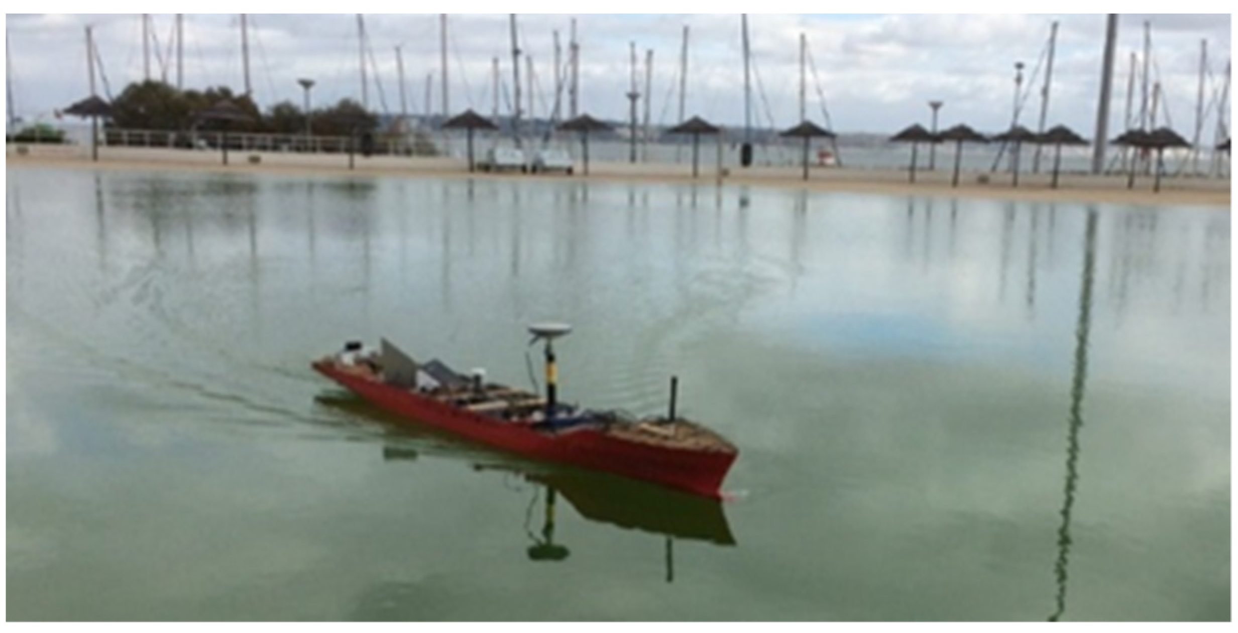
The vessel model used in the free-running test was a scaled container (Figure 1) with its main dimensions given in

Table 1. Main dimensions of the container model.

Length (m)	3.24
Breadth (m)	0.43
Draught (estimated at the tests) (m)	0.14
Model mass (kg)	108.58
Water depth (m)	0.185
Propeller diameter (m)	0.10

. The ship model had one propeller and one rudder in the aft.

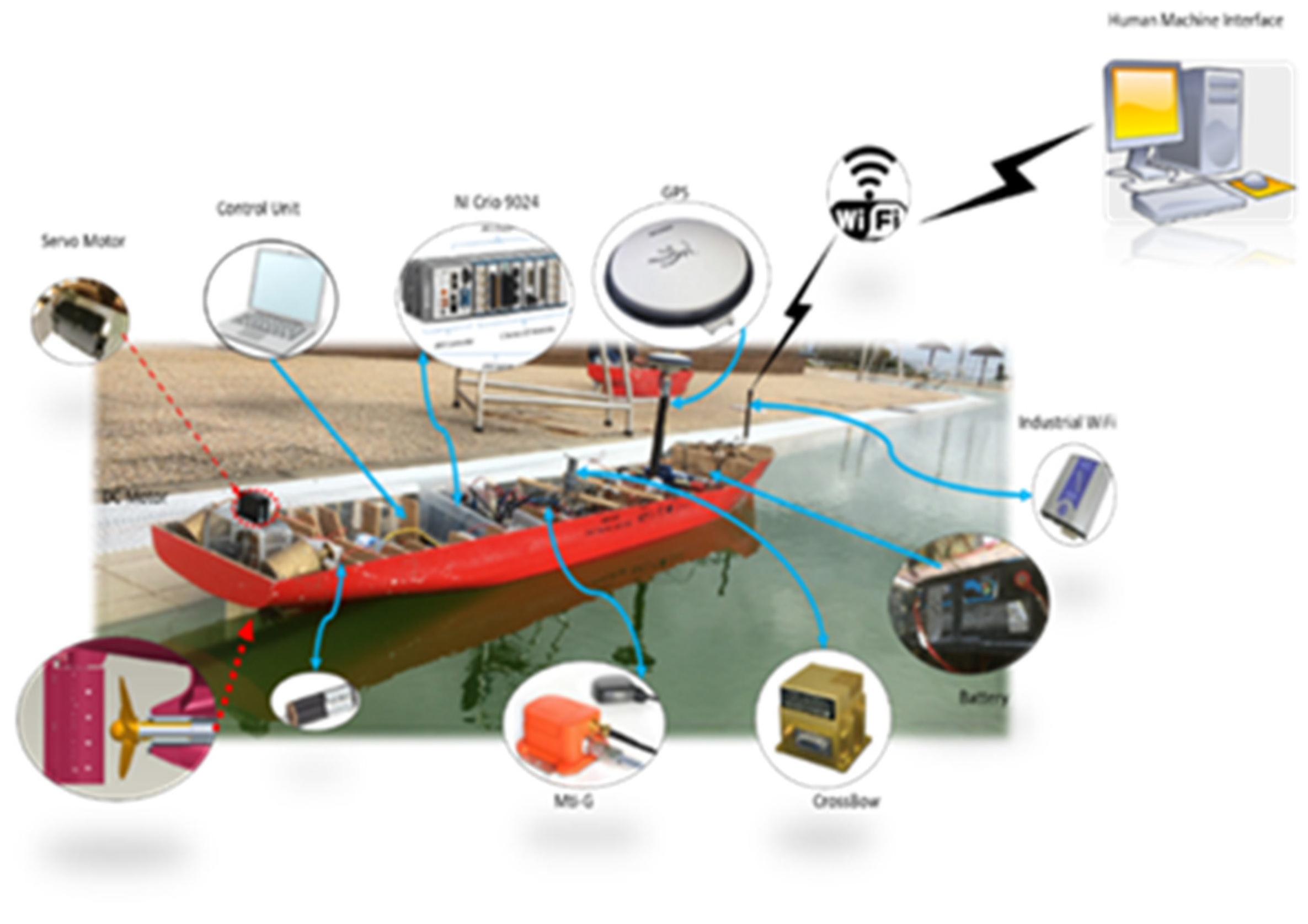
The hardware system of the free-running ship model consisted of all the sensors and actuators, as illustrated in Figure 2. The hardware system was further divided into two groups: on-board and onshore control centre. The on-board system was composed of a propeller, a rudder and set of sensors, an internal measurement unit, a yaw rate sensor, electrical motors, and an industrial Wi-Fi unit, where all the signals were synchronised using a Compact-RIO and stored in a laptop. This was used to control the self-running model remotely [33,34].

The software architecture was mainly programmed by LABVIEW software. The software architecture consisted of several program loops: an FPGA loop, real-time loop, and TCP/IP loop. It was used to collect data from the sensors (e.g., GPS, IMU) and to control the actuation of the propeller and rudder sub-systems that were programmed under a reconfigurable FPGA platform in LABVIEW. The sensor data were incorporated into network shared variables that were predicted along the entire network.

The zigzag manoeuvring test was carried out successfully through several repetitions. The ones that were analysed were a 20°−20° zigzag manoeuvre and the first and second repetition of a 30°−30° zigzag manoeuvre.

4. Optimal Parameter Estimation Method

To compute the hydrodynamic coefficients, the least squares method was firstly to diminish the error of the squared residual value, r, minimizing the sum, S, of the squared difference between the data value, $y_i$, and the estimation ($\widehat{y_i})$:

$$S={\displaystyle \sum }_{i=1}^n{r}_i^2={\displaystyle \sum }_{i=1}^n{\left(y_i-\widehat{y_i}\right)}^2$$

(13)

In the case of the hydrodynamic coefficients, Equation (2), can be written as follows:

$$\mathit{Y}=\mathit{X}\mathit{\theta }$$

(14)

where the vector Y represents the outputs, the matrix X represents the inputs, and the vector θ represents the values of the wanted parameters.

Considering the variance of the coefficients, a weighted sum of squared residual error, known as the chi-squared, was calculated:

$${\mathit{\chi }}^2\left(\mathit{\theta }\right)={(\mathit{X}\mathit{\theta }-\mathit{y})}^{\mathit{T}}{\mathit{V}}_{\mathit{y}}^{-1}{(\mathit{X}\mathit{\theta }-\mathit{y})}^{\mathit{T}}$$

(15)

To find the minimum error, the derivative of ${\mathit{\chi }}^2$ needs to be zero (Equations (16) and (17)) when the parameter θ is equal to the estimated one.

$${\frac{\partial {\mathit{\chi }}^2}{\partial \mathit{\theta }}}_{|\mathit{\theta }=\widehat{\mathit{\theta }}}=0\iff {\mathit{X}}^{\mathit{T}}{\mathit{V}}_{\mathit{y}}^{-1}\mathit{X}\widehat{\mathit{\theta }}-{\mathit{X}}^{\mathit{T}}{\mathit{V}}_{\mathit{y}}^{-1}\mathit{y}=0$$

(16)

$$\widehat{\mathit{\theta }}={\left[{\mathit{X}}^{\mathit{T}}{\mathit{V}}_{\mathit{y}}^{-1}\mathit{X}\right]}^{-1}{\mathit{X}}^{\mathit{T}}{\mathit{V}}_{\mathit{y}}^{-1}\mathit{y}$$

(17)

Secondly, the singular value decomposition method was applied to help the LSM deal with the multicollinearity and parameter drift problems. SVD uses the singular values of the input matrix to diagonalise it with the singular values:

$$\mathit{X}=\mathit{U}\Sigma {\mathit{V}}^{\mathit{T}}$$

(18)

In Equation (18), the general formulation of the SVD of the matrix X is expressed as being dependent on the orthonormal bases for the column space, the orthonormal base for the rows, and the descending sorted diagonal matrix of the singular values (U, V, and $\Sigma$ respectively).

Finally, to deal with a large number of adjustment coefficients, the truncated singular value decomposition, eliminating the smallest singular values of the input matrix, was applied. It reduces the initial rank, n, of the input matrix X and constructs a new input matrix ${\mathit{X}}_k$ with k rows, corresponding to the k singular values that were kept:

$${\mathit{X}}_k={\mathit{U}}_k{\Sigma }_k{\mathit{V}}_k^{\mathit{T}}$$

(19)

where ${\mathit{\Sigma }}_k$ is a diagonal matrix where the smaller n-k singular values are replaced by zeros [35]. Thus, it can diminish the uncertainty due to the multicollinearity and parameter drift problems, providing better results. When n is equal to k the result will be the same as that of LSM with only SVD.

The uncertainty of the coefficients can be given by the error propagation matrix ${\mathit{V}}_{\widehat{\mathit{\theta }}}$ [28]. This matrix defines how the optimal parameter varies with the output measured data.

$${\mathit{V}}_{\widehat{\mathit{\theta }}}=\left[\frac{\partial \widehat{\mathit{\theta }}}{\partial y}\right]{\mathit{V}}_y{\left[\frac{\partial \widehat{\mathit{\theta }}}{\partial y}\right]}^{\mathit{T}}$$

(20)

The square-root of ${\mathit{V}}_{\widehat{\mathit{\theta }}}$ gives the standard error of the parameters.

5. Parameter Estimation of the Manoeuvring Model and Sensitivity Analysis

The identification and validation of the estimation of hydrodynamic coefficients were carried out by using manoeuvres either simulated or from free-running tests. The chosen manoeuvres were a turning test and zig-zag manoeuvre tests, both for simulation purposes and only the zig-zag manoeuvres for the free-running tests.

It is essential to know how the rudder behaves in both manoeuvres. The rudder order is given by Equation (21) to the turning manoeuvre and Equation (22) to the zig-zag manoeuvre:

$${\delta }^{*}\left(radians\right)=\frac{{\delta }^{*}\left(degrees\right)\times \pi }{180}$$

(21)

$${\delta }^{*}={\delta }_{z}sign\left({\psi }_{z}signr-\psi \right)$$

(22)

where ${\delta }^{*}$ is the rudder order, ${\delta }_z$ is the fixed rudder angle in radians (equivalent to 20° or 30° depending on the zigzag analysed), and ${\psi }_z$ is a fixed heading angle in radians (equivalent to 20° or 30° depending on the zigzag analysed).

For the simulation of the 25° turning manoeuvre and the 20°−20° zigzag manoeuvre, the adjustment coefficients were initially taken as unitary to perform the manoeuvres. They were both run for 1000 s, with a time step of 0.01 s. The initial conditions were the same as in the free-running tests:

$$initial conditions=\left[u v r \eta \xi \psi {\delta }_R\right]=\left[0.96 0 0 0 0 0 0\right]$$

(23)

where the velocities are all in meters per second. The rudder angle is as in Equation (9). The horizontal and vertical position of the centre of mass of the ship are η and ξ, respectively, depending on the heading angle ψ:

$$\{\begin{array}{c}\dot{\eta }=ucos\left(\psi \right)-vsin\left(\psi \right)\\ \dot{\xi }=ucos\left(\psi \right)+vsin\left(\psi \right)\\ \dot{\psi }=r\end{array}$$

(24)

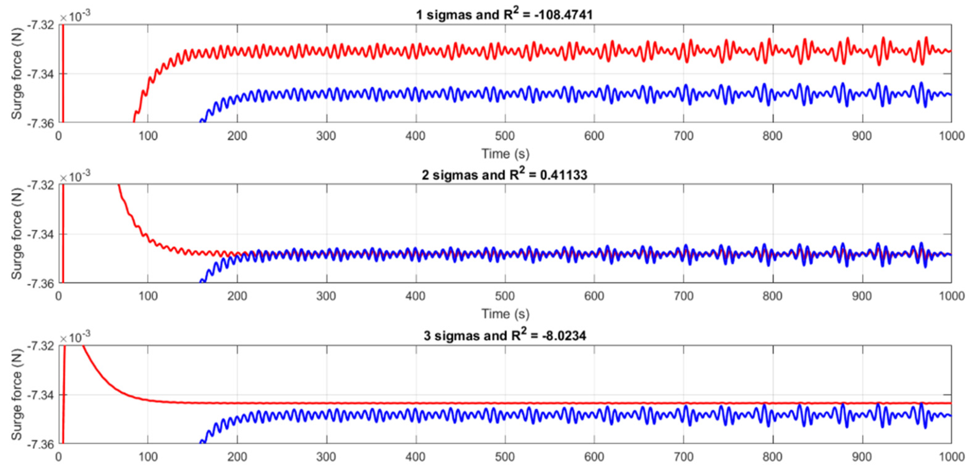
5.1. Identification and Validation Using Simulation Data

With the surge motion having just three coefficients, meaning at maximum three singular values, the results are very easy to read. Even with a coefficient of determination slightly smaller than 0.5, the results regarding this and the uncertainties were better when two singular values were considered (

Table 2. Surge adjustment coefficients and uncertainties for simulation of 25° turning manoeuvres.

	Surge
	k = 1		k = 2		k = 3
	Coefficients	Uncertainties	Coefficients	Uncertainties	Coefficients	Uncertainties
$k_{xuu}$	7.276 × 10−3	0.041%	9.543 × 10−1	0.561%	1.255	0.797%
$k_{xvr}$	−7.187 × 10−2	0.041%	3.084 × 10−2	1.885%	3.497 × 10−3	27.543%
$k_{x\delta \delta }$	2.688 × 10−3	0.041%	1.850 × 10−1	0.557%	−1.359	3.203%
	$R^2$	−108.4741	$R^2$	0.41133	$R^2$	−8.0234

and Figure 3). In Figure 3, Figure 4, Figure 5, Figure 6, Figure 7, Figure 8, Figure 9, Figure 10, Figure 11, Figure 12, Figure 13 and Figure 14, the singular values are designated as “sigma”, the blue curves represent the measured forces and moments, and the red curves represent the estimated forces and moments.

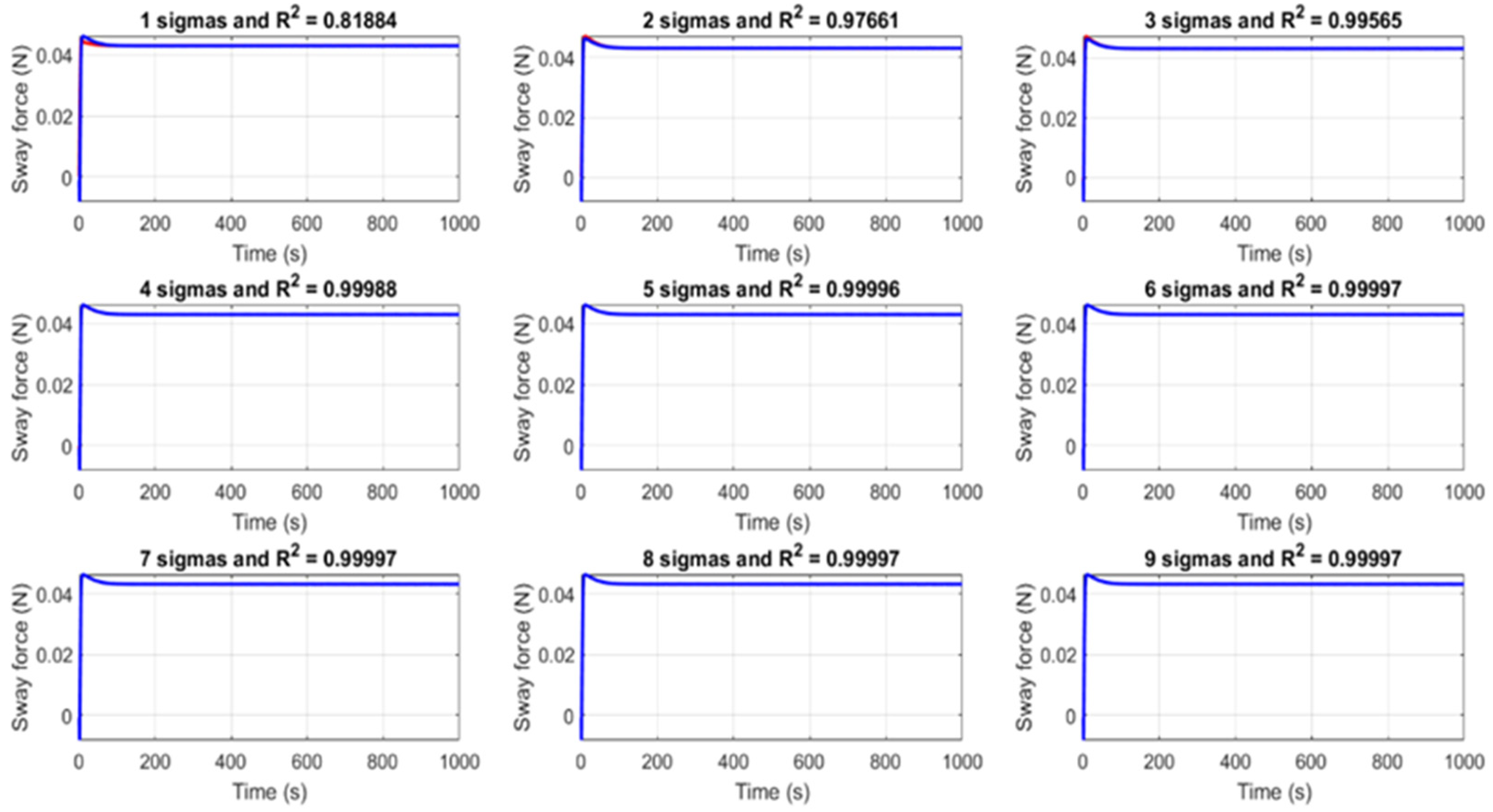
For both sway and yaw motions, the identified results agreed very well with the training set, where the coefficient of determination was almost equal to 1 (Figure 4 and Figure 5). The obtained adjustment coefficients (

Table 3. Sway adjustment coefficients and uncertainties for simulation of 25° turning manoeuvre.

	Sway
	k = 1		k = 2		k = 3
	Coefficients	Uncertainties	Coefficients	Uncertainties	Coefficients	Uncertainties
$k_{y0}$	−1.809 × 10−5	0.007%	2.046 × 10−5	0.229%	4.983 × 10−2	0.151%
$k_{yv}$	6.22 × 10−4	0.007%	1.657 × 10−3	0.076%	−1.040 × 10−1	0.153%
$k_{yr}$	2.835 × 10−2	0.007%	6.762 × 10−3	0.389%	2.954 × 10−2	0.123%
$k_{yvvv}$	4.218 × 10−5	0.007%	2.405 × 10−4	0.100%	−2.274 × 10−2	0.153%
$k_{yvvr}$	1.304 × 10−2	0.007%	5.998 × 10−2	0.095%	5.447 × 10−2	0.048%
$k_{y\delta }$	−5.757 × 10−4	0.007%	4.056 × 10−4	0.295%	8.794 × 10−1	0.151%
$k_{yvv\delta }$	−2.610 × 10−5	0.007%	−1.181 × 10−4	0.095%	5.331 × 10−3	0.154%
$k_{yv\delta \delta }$	3.520 × 10−7	0.007%	9.907 × 10−7	0.079%	1.504 × 10−6	0.056%
$k_{y\delta \delta \delta }$	1.809 × 10−5	0.007%	−2.912 × 10−6	0.878%	−9.548 × 10−3	0.151%
	$R^2$	0.81884	$R^2$	0.97661	$R^2$	0.99565
	k = 4		k = 5		k = 6
	Coefficients	Uncertainties	Coefficients	Uncertainties	Coefficients	Uncertainties
$k_{y0}$	9.806 × 10−2	0.029%	1.445	0.212%	1.224	0.273%
$k_{yv}$	1.189	0.057%	1.133	0.037%	1.119	0.036%
$k_{yr}$	2.075 × 10−2	0.036%	2072 × 10−2	0.021%	2.156 × 10−2	0.036%
$k_{yvvv}$	2.748 × 10−3	0.527%	4.178 × 10−1	0.226%	1.064	0.489%
$k_{yvvr}$	1.848 × 10−2	0.104%	1.830 × 10−2	0.062%	1.570 × 10−2	0.148%
$k_{y\delta }$	1.033	0.022%	9.636 × 10−1	0.022%	9.933 × 10−1	0.031%
$k_{yvv\delta }$	−3.965 × 10−2	0.059%	−8.395 × 10−2	0.121%	−1.849 × 10−1	0.437%
$k_{yv\delta \delta }$	8.340 × 10−4	0.052%	5.111 × 10−4	0.152%	6.189 × 10−4	0.181%
$k_{y\delta \delta \delta }$	1.856 × 10−2	0.080%	2.239 × 10−1	0.208%	3.505 × 10−1	0.312%
	$R^2$	0.99988	$R^2$	0.99996	$R^2$	0.99997
	k = 7		k = 8		k = 9
	Coefficients	Uncertainties	Coefficients	Uncertainties	Coefficients	Uncertainties
$k_{y0}$	1.140	0.341%	1.138	0.343%	1.154	0.546%
$k_{yv}$	1.110	0.041%	1.195	1.207%	1.130	2.149%
$k_{yr}$	2.103 × 10−2	0.071%	2.073 × 10−2	0.256%	2.068 × 10−2	0.267%
$k_{yvvv}$	8.698 × 10−1	0.803%	1.330	5.872%	1.244	6.618%
$k_{yvvr}$	1.715 × 10−2	0.245%	1.788 × 10−2	0.723%	1.799 × 10−2	0.744%
$k_{y\delta }$	1.001	0.036%	1.005	0.064%	9.970 × 10−1	0.241%
$k_{yvv\delta }$	−1.206 × 10−2	35.311%	2.488	16.997%	2.107	20.811%
$k_{yv\delta \delta }$	1.478 × 10−4	7.748%	1.309 × 10−2	16.723%	7.959 × 101	30.335%
$k_{y\delta \delta \delta }$	1.331	1.784%	9.824 × 10−1	6.476%	1.072	6.452%
	$R^2$	0.99997	$R^2$	0.99997	$R^2$	0.99997

and

Table 4. Yaw adjustment coefficients and uncertainties for simulation of 25° turning manoeuvre.

	Yaw
	k = 1		k = 2		k = 3
	Coefficients	Uncertainties	Coefficients	Uncertainties	Coefficients	Uncertainties
$k_{n0}$	1.223 × 10−6	0.335%	1.236 × 10−4	0.304%	2.882 × 10−1	0.024%
$k_{nv}$	9.849 × 10−6	0.335%	−1.036 × 10−3	0.310%	1.277 × 10−1	0.024%
$k_{nr}$	−1.234 × 10−3	0.335%	−3.271 × 10−2	0.295%	5.712 × 10−2	0.039%
$k_{nvvv}$	−7.841 × 10−7	0.335%	2.122 × 10−4	0.308%	−3.572 × 10−2	0.024%
$k_{nvvr}$	−4.287 × 10−4	0.335%	9.031 × 10−2	0.308%	4.621 × 10−2	0.050%
$k_{n\delta }$	2.640 × 10−5	0.335%	2.055 × 10−3	0.303%	3.422	0.024%
$k_{nvv\delta }$	−9.882 × 10−7	0.335%	2.042 × 10−4	0.308%	−1.623 × 10−2	0.024%
$k_{nv\delta \delta }$	−1.065 × 10−7	0.335%	1.210 × 10−5	0.310%	1.839 × 10−4	0.022%
$k_{n\delta \delta \delta }$	−8.202 × 10−7	0.335%	−3.959 × 10−5	0.300%	−3.584 × 10−2	0.024%
	$R^2$	−0.055445	$R^2$	0.48834	$R^2$	0.99717
	k = 4		k = 5		k = 6
	Coefficients	Uncertainties	Coefficients	Uncertainties	Coefficients	Uncertainties
$k_{n0}$	1.635 × 10−1	0.705%	3.248	0.291%	2.788	0.367%
$k_{nv}$	8.500 × 10−1	0.784%	1.397	0.352%	1.700	0.333%
$k_{nr}$	5.910 × 10−2	0.047%	5.773 × 10−2	0.034%	5.958 × 10−2	0.045%
$k_{nvvv}$	−5.669 × 10−2	0.342%	1.185 × 10−1	0.466%	3.980	1.008%
$k_{nvvr}$	5.596 × 10−2	0.165%	6.351 × 10−2	0.108%	5.549 × 10−2	0.191%
$k_{n\delta }$	3.405	0.023%	3.129	0.032%	3.228	0.044%
$k_{nvv\delta }$	−7.717 × 10−2	0.729%	−8.685 × 10−2	0.451%	1.043	1.126%
$k_{nv\delta \delta }$	−8.566 × 10−3	0.942%	−1.843 × 10−2	0.345%	−1.690 × 10−2	0.372%
$k_{n\delta \delta \delta }$	−8.549 × 10−2	0.536%	1.602 × 10−1	0.509%	2.669	0.977%
	$R^2$	0.99747	$R^2$	0.99875	$R^2$	0.99886
	k = 7		k = 8		k = 9
	Coefficients	Uncertainties	Coefficients	Uncertainties	Coefficients	Uncertainties
$k_{n0}$	2.780	0.411%	2.781	0.413%	2.461	0.752%
$k_{nv}$	1.702	0.346%	1.759	10.234%	−3.663	8.333%
$k_{nr}$	5.948 × 10−2	0.118%	5.956 × 10−2	0.409%	6.107 × 10−2	0.413%
$k_{nvvv}$	3.901	1.770%	3.639	22.940%	9.876	8.910%
$k_{nvvr}$	5.583 × 10−2	0.465%	5.559 × 10−2	1.411%	5.106 × 10−2	1.584%
$k_{n\delta }$	3.229	0.048%	3.228	0.085%	3.449	0.302%
$k_{nvv\delta }$	9.969 × 10−1	3.501%	1.696	130.957%	−1.197 × 101	19.230%
$k_{nv\delta \delta }$	−1.760 × 10−2	2.846%	−5.124 × 10−2	208.506%	−3.483 × 102	4.553%
$k_{n\delta \delta \delta }$	2.810	3.683%	2.892	9.614%	2.462 × 10−1	123.107
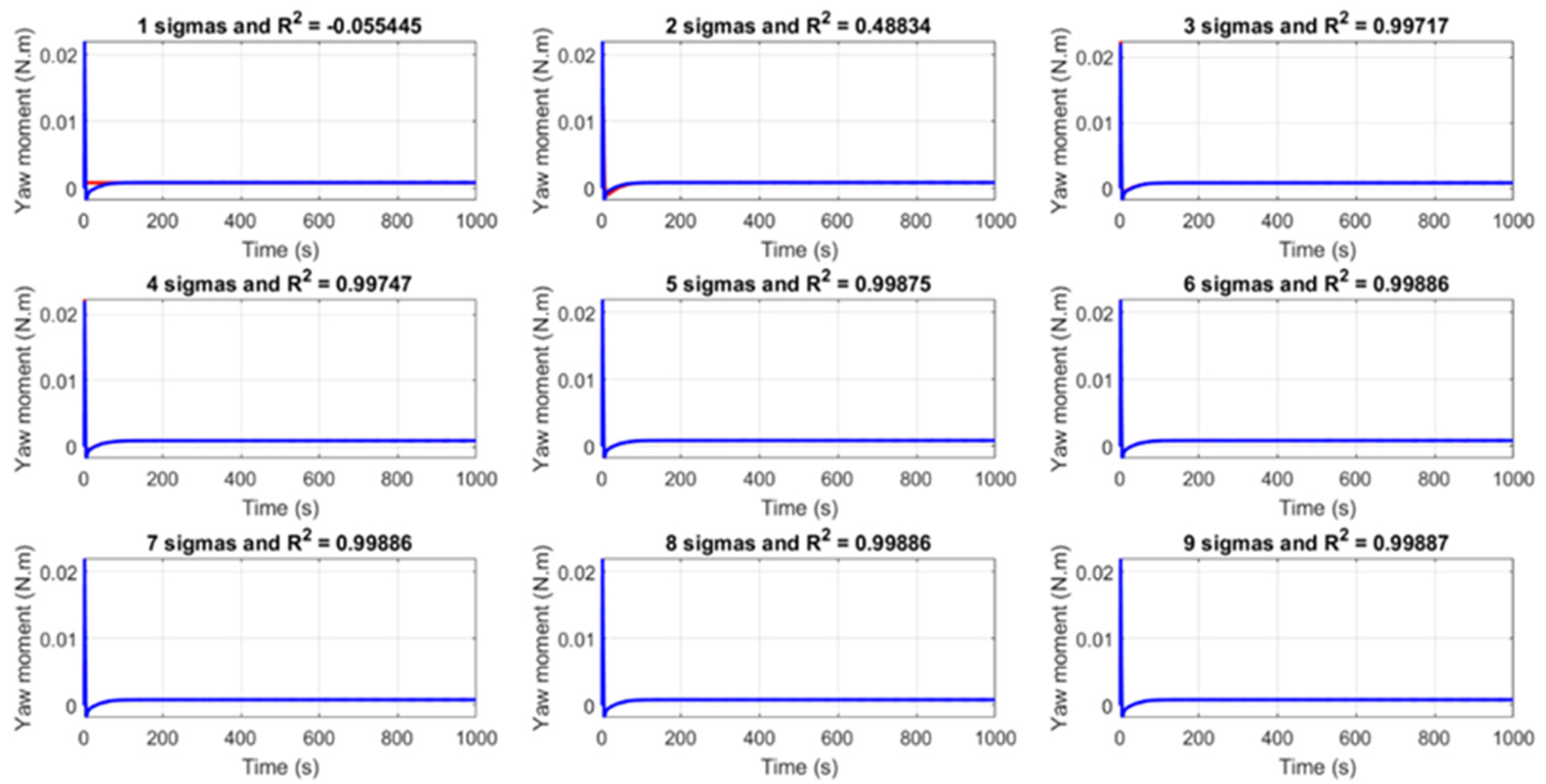
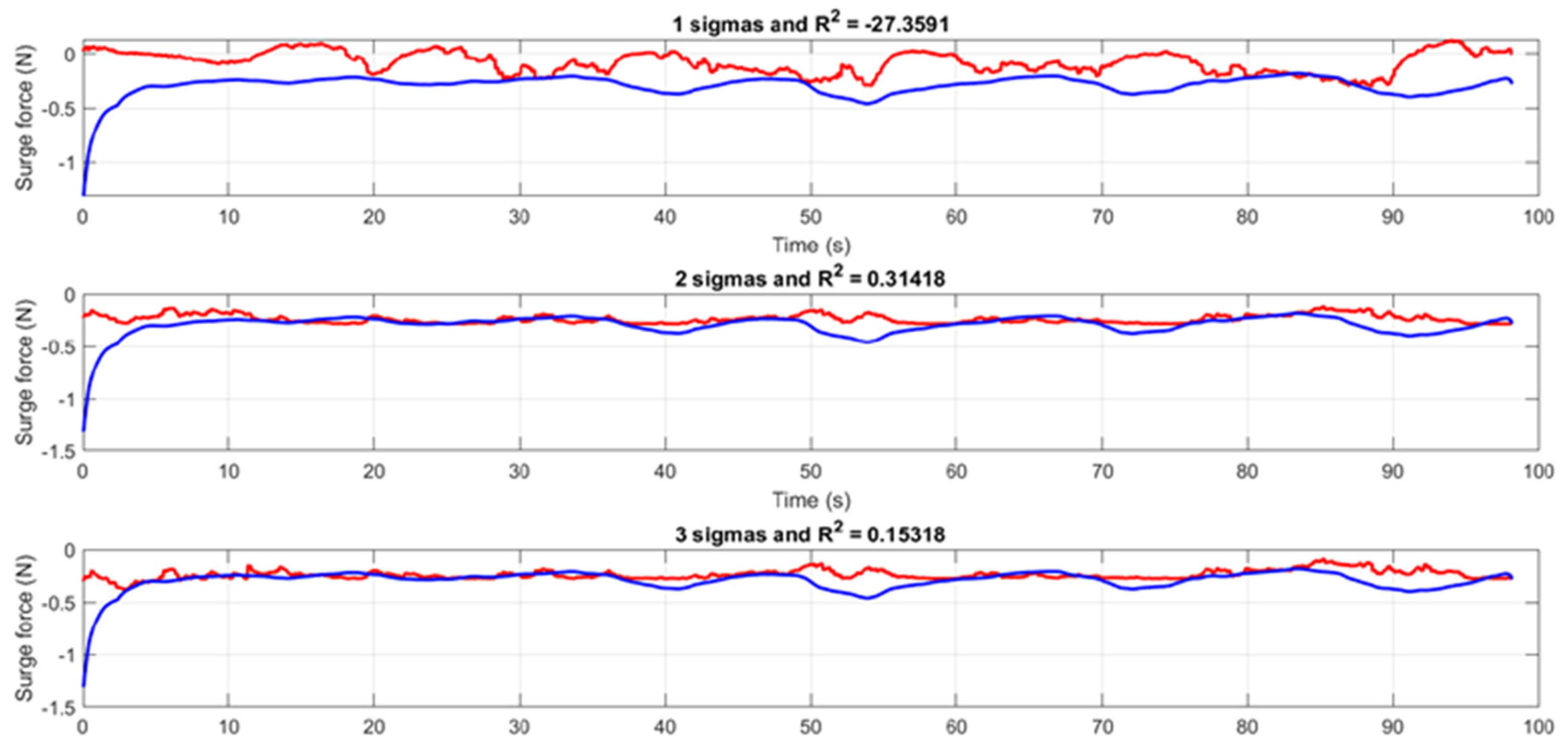
	$R^2$	0.99886	$R^2$	0.99886	$R^2$	0.99887

) were very close with the true values in the simulation when we kept more than six singular values (k ≥ 6). The parameter uncertainties increased with the numbers of singular values, which indicated that the noise effect was amplified when keeping more singular values. Therefore, the truncated value, k, plays a trade-off role between the accuracy of the identified parameter and uncertainty due to the noise. This is obvious as the uncertainties of the results for one singular value (k = 1) were very small, but the results were the farthest from unitary, showing signals of parameter drift. The least squares method combined with the truncated singular value decomposition was valuable considering the parameter uncertainties. It is important to note that noise was not added to the data generated by the simulation. The validation for surge, sway and yaw motion was carried out using 20°–20° zigzag manoeuvre simulation test, and the results are presented in Figure 6, Figure 7 and Figure 8.

5.2. Identification and Validation Using Free-Running Tests

The identification was performed using the first and second repetition data from tests of a 30°–30° zigzag manoeuvre and the validation with data from a 20°–20° zigzag manoeuvre test.

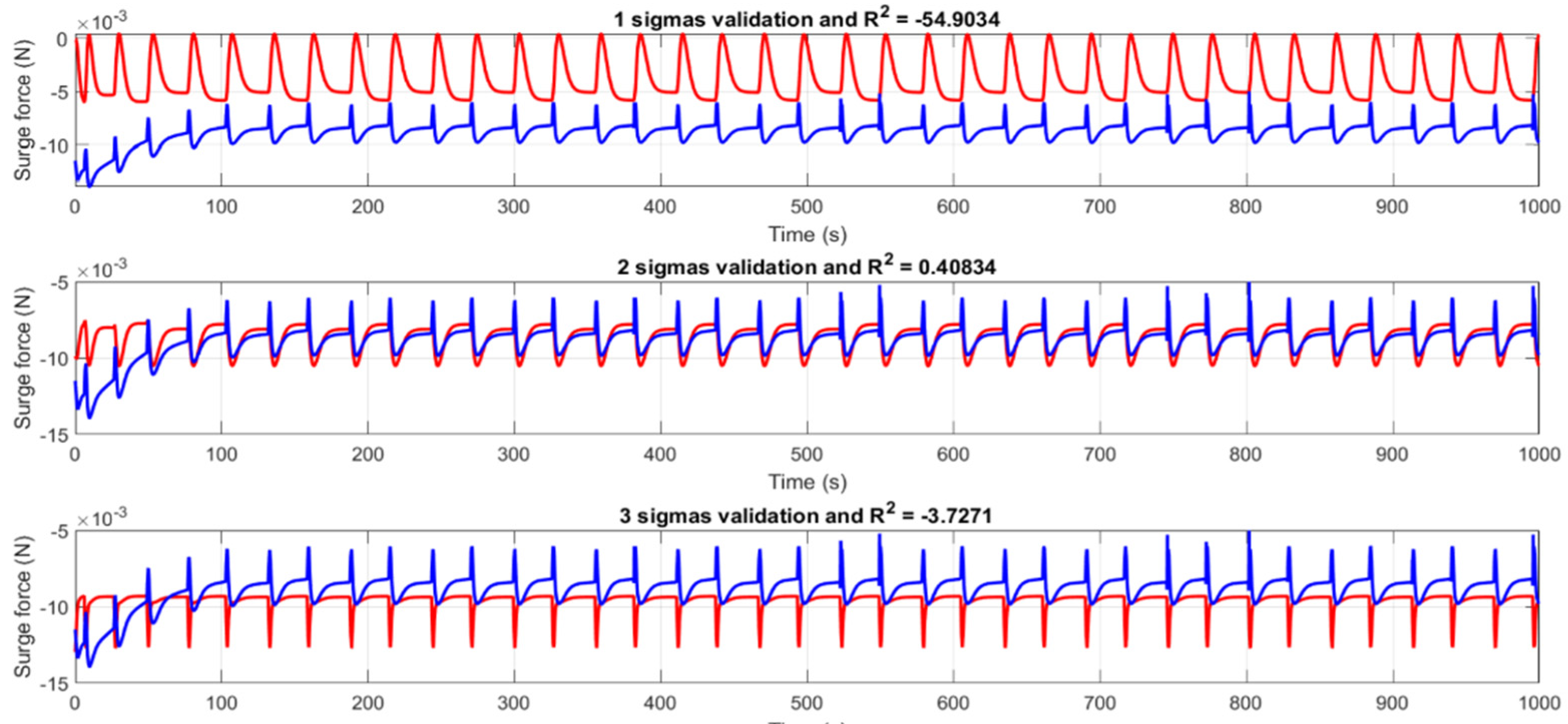
Concerning the surge motion, once again the adjustment coefficients were better for the two singular value results when considering the correlation between the uncertainties and the coefficient of determination between the measured and estimated forces (

Table 5. Surge adjustment coefficients and uncertainties for tests’ data from the 30°−30° zigzag manoeuvre.

	Surge
	k = 1		k = 2		k = 3
	Coefficients	Uncertainties	Coefficients	Uncertainties	Coefficients	Uncertainties
$k_{xuu}$	3.214 × 10−3	4.022%	2.730 × 101	1.224%	3.724 × 101	2.405%
$k_{xvr}$	−2.853 × 10−1	4.022%	2.220 × 10−2	29.853%	−1.237 × 10−2	56.814%
$k_{x\delta \delta }$	6.360 × 10−7	4.022%	4.128 × 10−3	1.224%	−6.575 × 104	8.405%
	$R^2$	−27.3591	$R^2$	0.31418	$R^2$	0.15318

and Figure 9).

For the sway motion, the best results were for the six and seven singular values regarding the uncertainties (

Table 6. Sway adjustment coefficients and uncertainties for tests’ data from the 30°−30° zigzag manoeuvre.

	Sway
	k = 1		k = 2		k = 3
	Coefficients	Uncertainties	Coefficients	Uncertainties	Coefficients	Uncertainties
$k_{y0}$	4.651 × 10−8	5.152%	−6.071 × 10−6	10.531%	2.957 × 10−4	5.719%
$k_{yv}$	1.352 × 10−5	5.152%	6.461 × 10−4	10.233%	6.952 × 10−2	5.550%
$k_{yr}$	4.205 × 10−4	5.152%	4.097 × 10−2	10.344%	4.039 × 10−2	9.601%
$k_{yvvv}$	3.165 × 10−5	5.152%	−7.410 × 10−5	15.068%	2.212 × 10−1	5.603%
$k_{yvvr}$	6.379 × 10−3	5.152%	3.705 × 10−3	11.465%	2.499 × 10−3	15.786%
$k_{y\delta }$	−9.676 × 10−8	5.152%	−1.203 × 10−5	10.367%	1.280 × 10−4	6.192%
$k_{yvv\delta }$	−1.401 × 10−7	5.152%	−3.922 × 10−7	6.952%	3.102 × 10−4	5.608%
$k_{yv\delta \delta }$	3.402 × 10−12	5.152%	1.631 × 10−10	10.234%	1.710 × 10−8	5.548%
$k_{y\delta \delta \delta }$	1.344 × 10−12	5.152%	1.672 × 10−10	10.367%	−1.778 × 10−9	6.195%
	$R^2$	0.27838	$R^2$	0.38087	$R^2$
	k = 4		k = 5		k = 6
	Coefficients	Uncertainties	Coefficients	Uncertainties	Coefficients	Uncertainties
$k_{y0}$	4.969 × 10−3	12.545%	−7.890 × 101	8.337%	−4.502 × 101	13.674%
$k_{yv}$	7.417 × 10−1	12.095%	1.260	7.640%	9.223 × 10−1	9.563%
$k_{yr}$	2.939 × 10−2	13.906%	1.293 × 10−2	31.106%	6.747 × 10−2	6.879%
$k_{yvvv}$	1.189 × 10−2	256.085%	−5.801 × 10−2	51.329%	−2.942 × 10−1	9.962%
$k_{yvvr}$	2.838 × 10−3	13.761%	4.063 × 10−3	9.553%	7.510 × 10−3	5.194%
$k_{y\delta }$	9.138 × 10−4	11.499%	1.223 × 101	8.336%	1.605 × 102	4.710%
$k_{yvv\delta }$	−3.636 × 10−4	25.156%	5.996	8.337%	1.495 × 102	4.867%
$k_{yv\delta \delta }$	1.572 × 10−7	11.899%	4.996 × 10−5	8.310%	3.830 × 10−4	4.507%
$k_{y\delta \delta \delta }$	−1.270 × 10−8	11.499%	−1.699 × 10−4	8.336%	−2.230 × 10−3	4.710%
	$R^2$	0.59526	$R^2$	0.72494	$R^2$	0.86986
	k = 7		k = 8		k = 9
	Coefficients	Uncertainties	Coefficients	Uncertainties	Coefficients	Uncertainties
$k_{y0}$	−4.215 × 101	14.899%	−4.177 × 101	15.022%	−4.177 × 101	71.599%
$k_{yv}$	8.347 × 10−1	11.544%	5.306 × 10−1	34.203%	2.845 × 101	58.440%
$k_{yr}$	8.035 × 10−2	9.199%	7.837 × 10−2	9.506%	3.193 × 10−1	46.229%
$k_{yvvv}$	−2.386 × 10−1	16.097%	−2.531 × 10−1	15.430%	1.227	73.321%
$k_{yvvr}$	6.246 × 10−3	10.986%	6.271 × 10−3	10.932%	4.750 × 10−3	71.380%
$k_{y\delta }$	1.988 × 102	9.409%	1.952 × 102	9.614%	2.769 × 1017	59.470%
$k_{yvv\delta }$	1.092 × 102	17.760%	1.095 × 102	17.701%	8.826 × 101	105.620%
$k_{yv\delta \delta }$	4.829 × 10−4	9.917%	1.446 × 106	50.576%	−1.360 × 108	60.157%
$k_{y\delta \delta \delta }$	−2.762 × 10−3	9.409%	−2.713 × 10−3	9.614%	1.993 × 1022	59.470%
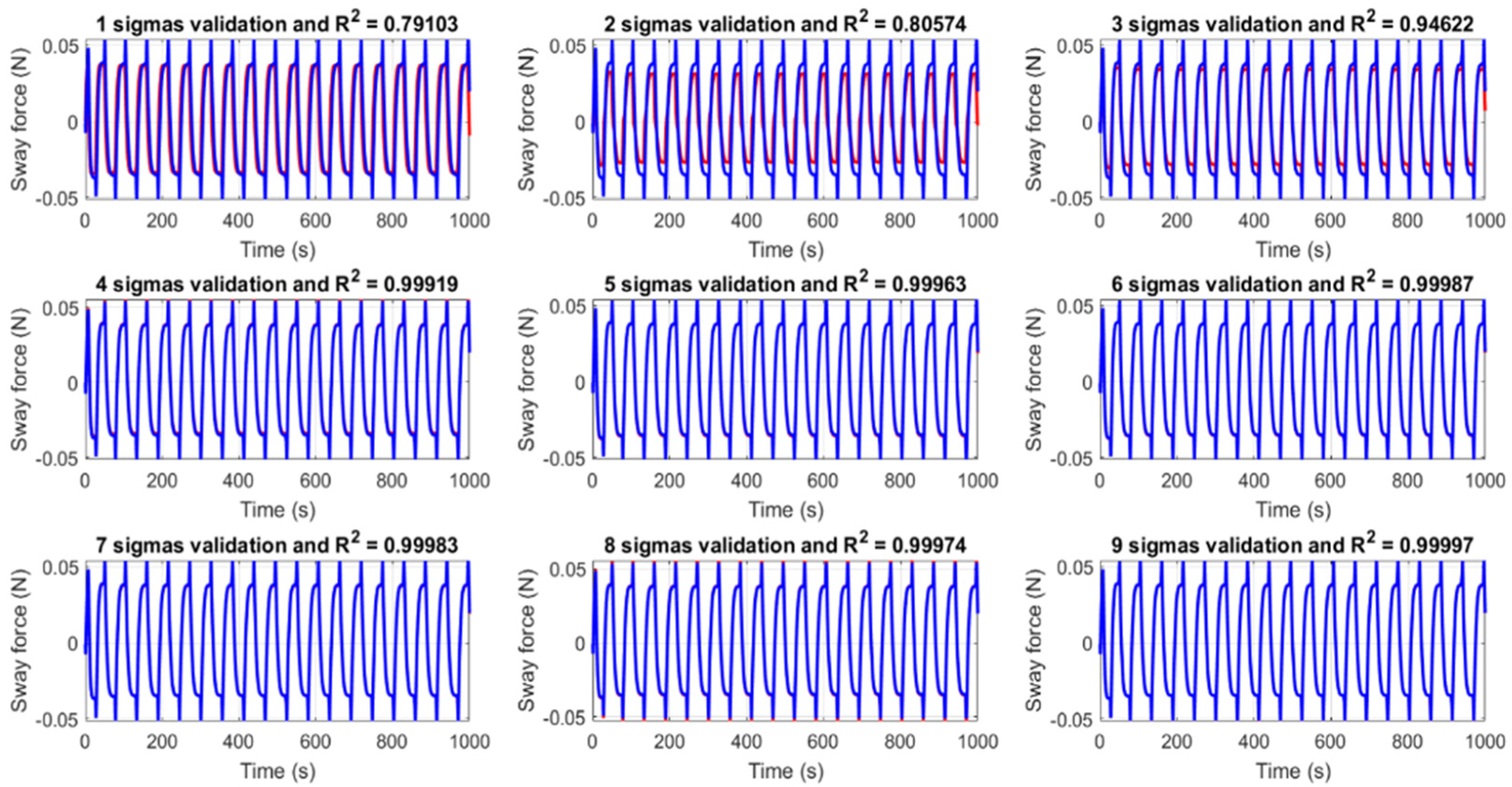
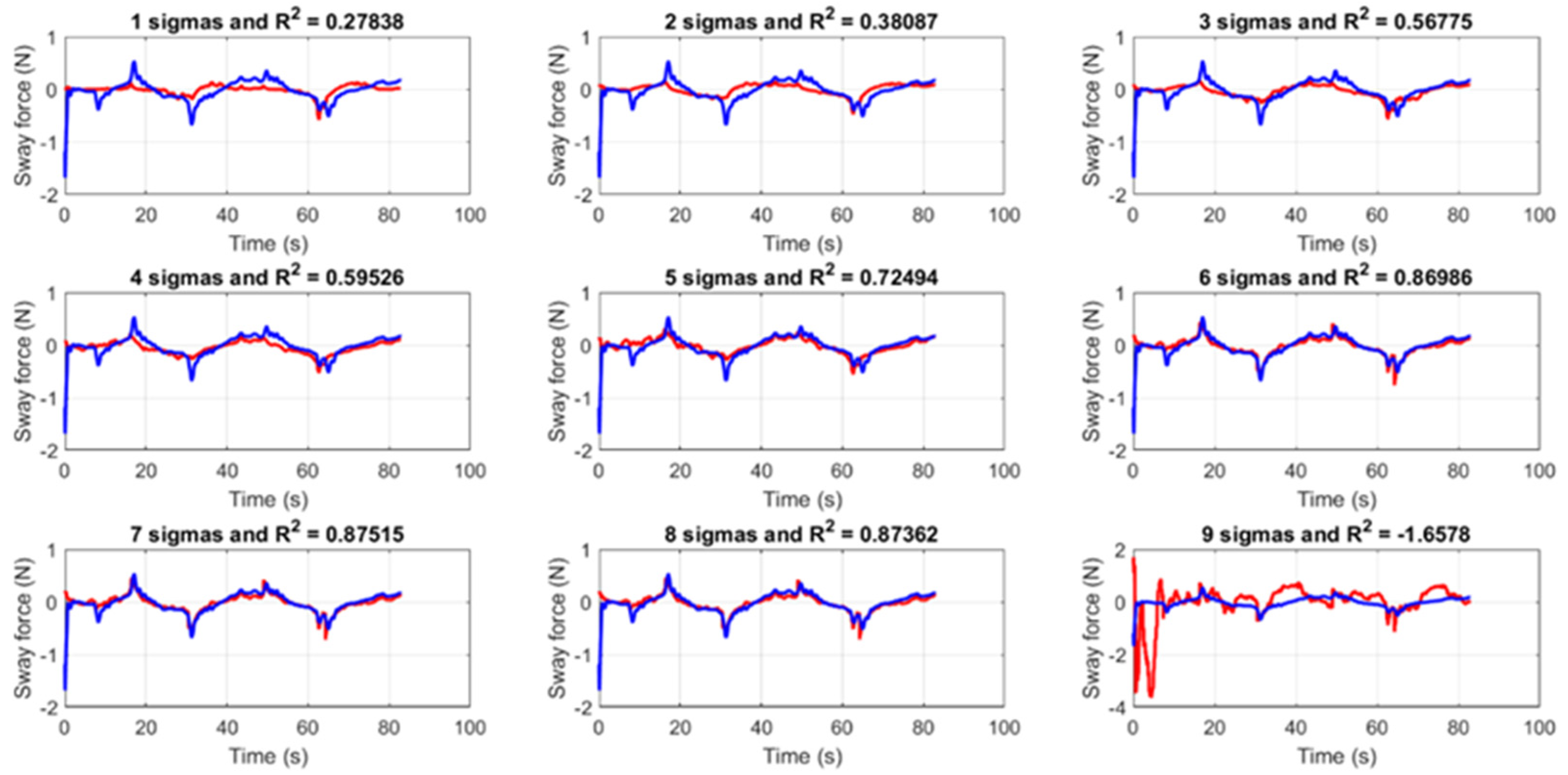
	$R^2$	0.87515	$R^2$	0.87362	$R^2$	−1.6578

). The measured and estimated forces were also well fitted for the six and seven singular values and the five and eight singular values (Figure 10). However, for these last two, some uncertainties had values that were higher than 50% and therefore not acceptable. Finally, the yaw motion was more constrained in good results. The only favourable ones were the results with six singular values, which had good uncertainties (

Table 7. Yaw adjustment coefficients and uncertainties for tests’ data from the 30°−30° zigzag manoeuvre.

	Yaw
	k = 1		k = 2		k = 3
	Coefficients	Uncertainties	Coefficients	Uncertainties	Coefficients	Uncertainties
$k_{n0}$	1.448 × 10−9	94.512%	1.038 × 10−6	20.883%	3.118 × 10−4	10.815%
$k_{nv}$	−9.929 × 10−8	94.512%	2.453 × 10−5	21.000%	−1.661 × 10−2	10.867%
$k_{nr}$	8.566 × 10−6	94.512%	−4.373 × 10−3	20.954%	−4.402 × 10−3	20.301%
$k_{nvvv}$	2.725 × 10−7	94.512%	5.969 × 10−6	20.412%	6.315 × 10−2	10.850%
$k_{nvvr}$	9.719 × 10−5	94.512%	4.834 × 10−4	25.204%	2.918 × 10−4	41.326%
$k_{n\delta }$	−2.068 × 10−9	94.512%	1.359 × 10−6	20.944%	9.947 × 10−5	10.707%
$k_{nvv\delta }$	2.459 × 10−9	94.512%	−1.800 × 10−8	27.007%	−1.806 × 10−4	10.850%
$k_{nv\delta \delta }$	4.780 × 10−13	94.512%	−1.185 × 10−10	21.000%	7.821 × 10−8	10.868%
$k_{n\delta \delta \delta }$	2.841 × 10−14	94.512%	−1.867 × 10−11	20.944%	−1.367 × 10−9	10.707%
	$R^2$	−0.00028577	$R^2$	0.049378	$R^2$	0.15467
	k = 4		k = 5		k = 6
	Coefficients	Uncertainties	Coefficients	Uncertainties	Coefficients	Uncertainties
$k_{n0}$	8.782 × 10−3	19.280%	−1.340 × 101	7.391%	−6.927	10.994%
$k_{nv}$	−3.034 × 10−1	18.901%	−6.862 × 10−1	8.934%	−3.383 × 10−1	13.839%
$k_{nr}$	−6.103 × 10−3	15.562%	−1.108 × 10−2	8.783%	1.112 × 10−2	8.572%
$k_{nvvv}$	−1.246 × 10−2	132.995%	−5.025 × 10−2	31.763%	−2.082 × 10−1	6.103%
$k_{nvvr}$	3.607 × 10−4	33.402%	7.484 × 10−4	15.741%	1.872 × 10−3	4.990%
$k_{n\delta }$	1.084 × 10−3	18.178%	1.166	7.379%	6.109 × 101	2.725%
$k_{nvv\delta }$	4.145 × 10−4	29.079%	−3.907 × 10−1	7.394%	−4.398 × 101	2.751%
$k_{nv\delta \delta }$	1.227 × 10−6	18.725%	3.682 × 10−5	7.164%	9.452 × 10−4	2.676%
$k_{n\delta \delta \delta }$	−1.489 × 10−8	18.178%	−1.602 × 10−5	7.379%	−8.393 × 10−4	2.725%
	$R^2$	0.2046	$R^2$	0.37128	$R^2$	0.77205
	k = 7		k = 8		k = 9
	Coefficients	Uncertainties	Coefficients	Uncertainties	Coefficients	Uncertainties
$k_{n0}$	−5.419	13.748%	−5.279	13.953%	−5.279	20.705%
$k_{nv}$	−1.227 × 10−1	39.828%	3.602 × 10−1	25.288%	3.736	22.084%
$k_{nr}$	2.259 × 10−2	6.033%	2.145 × 10−2	6.336%	4.927 × 10−3	90.642%
$k_{nvvv}$	−8.092 × 10−2	20.485%	−1.006 × 10−1	16.585%	−1.561 × 10−1	18.028%
$k_{nvvr}$	2.568 × 10−4	65.391%	2.761 × 10−4	60.120%	2.399 × 10−4	102.746%
$k_{n\delta }$	9.358 × 101	3.498%	9.163 × 101	3.547%	−4.912 × 1016	24.111%
$k_{nvv\delta }$	9.187 × 10−1	447.621%	7.646 × 10−1	531.527%	−3.305 × 10−1	1826.520%
$k_{nv\delta \delta }$	1.528 × 10−3	3.710%	1.200 × 105	15.989%	9.296 × 105	21.222%
$k_{n\delta \delta \delta }$	−1.286 × 10−3	3.498%	−1.259 × 10−3	3.547%	−3.575 × 10+21	24.111%
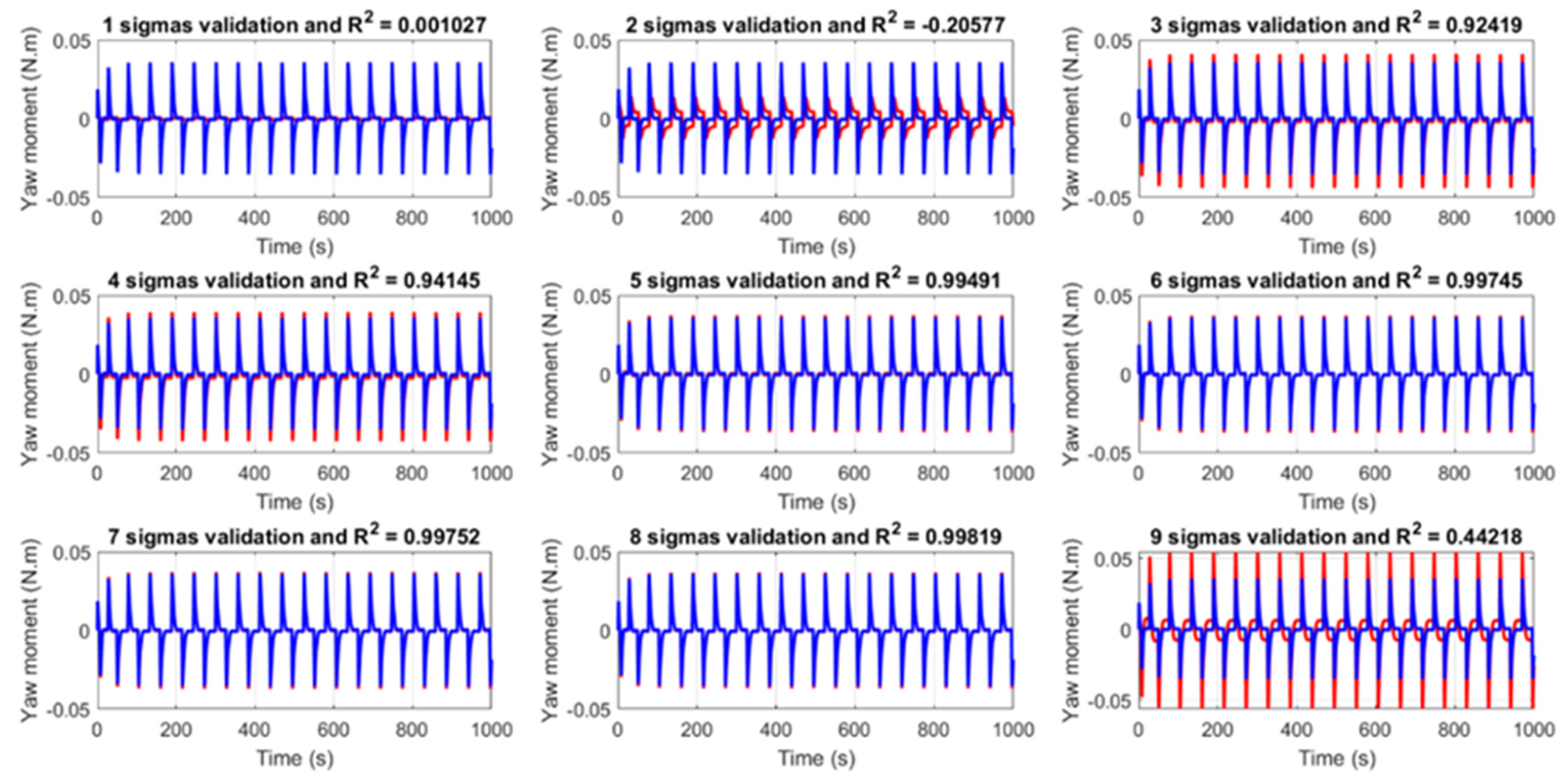
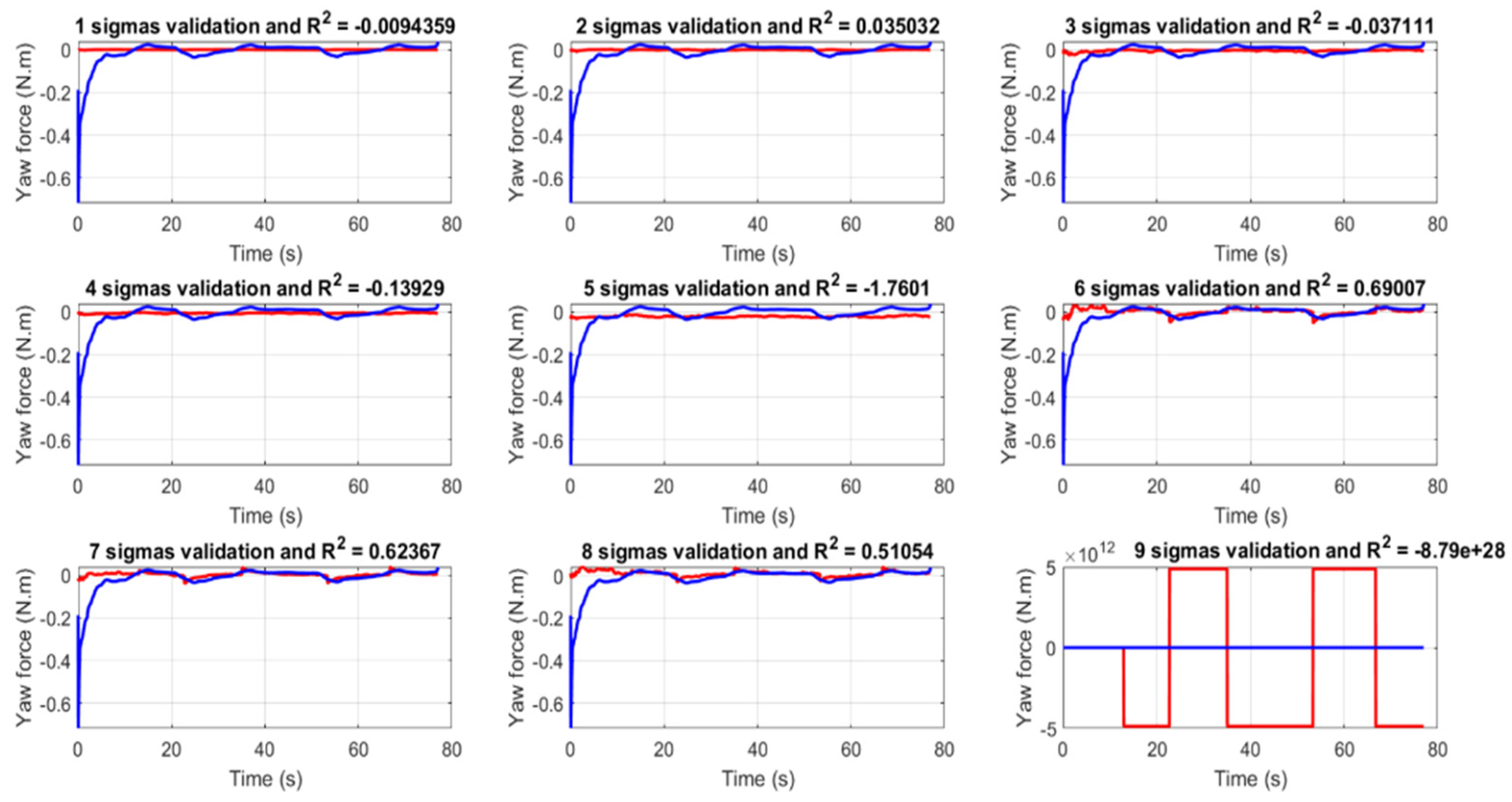
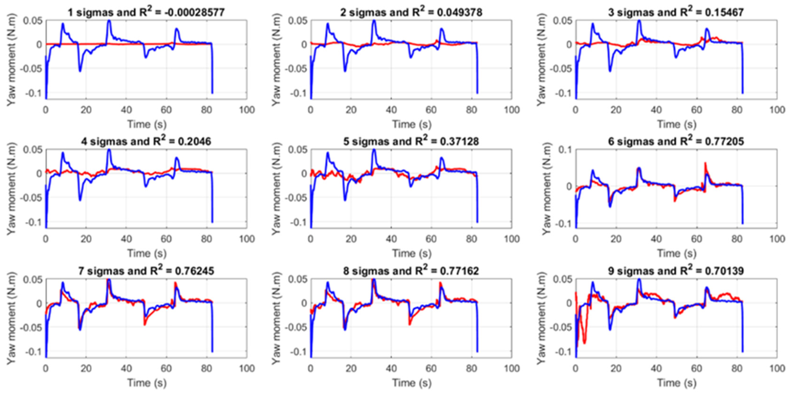
	$R^2$	0.76245	$R^2$	0.77162	$R^2$	0.70139

) and a good coefficient of determination between the measured and estimated yaw moments (Figure 11).

The results for the identification using test data were worse than those from the simulation because the noise was more significant in the real test data. The best results were for two singular values in surge motion and six singular values in sway and yaw motion. The major difference is that there were environmental surroundings when performing the free-running tests, such as waves and wind. There were no data for environmental disturbances and the manoeuvring model did not account for them. Hence, larger uncertainties and smaller coefficients of determination were the achieved results. Nonetheless, it was proved that the addition of the TSVD was helpful to obtain better coefficients, fighting multicollinearity regarding the large number of coefficients to be computed.

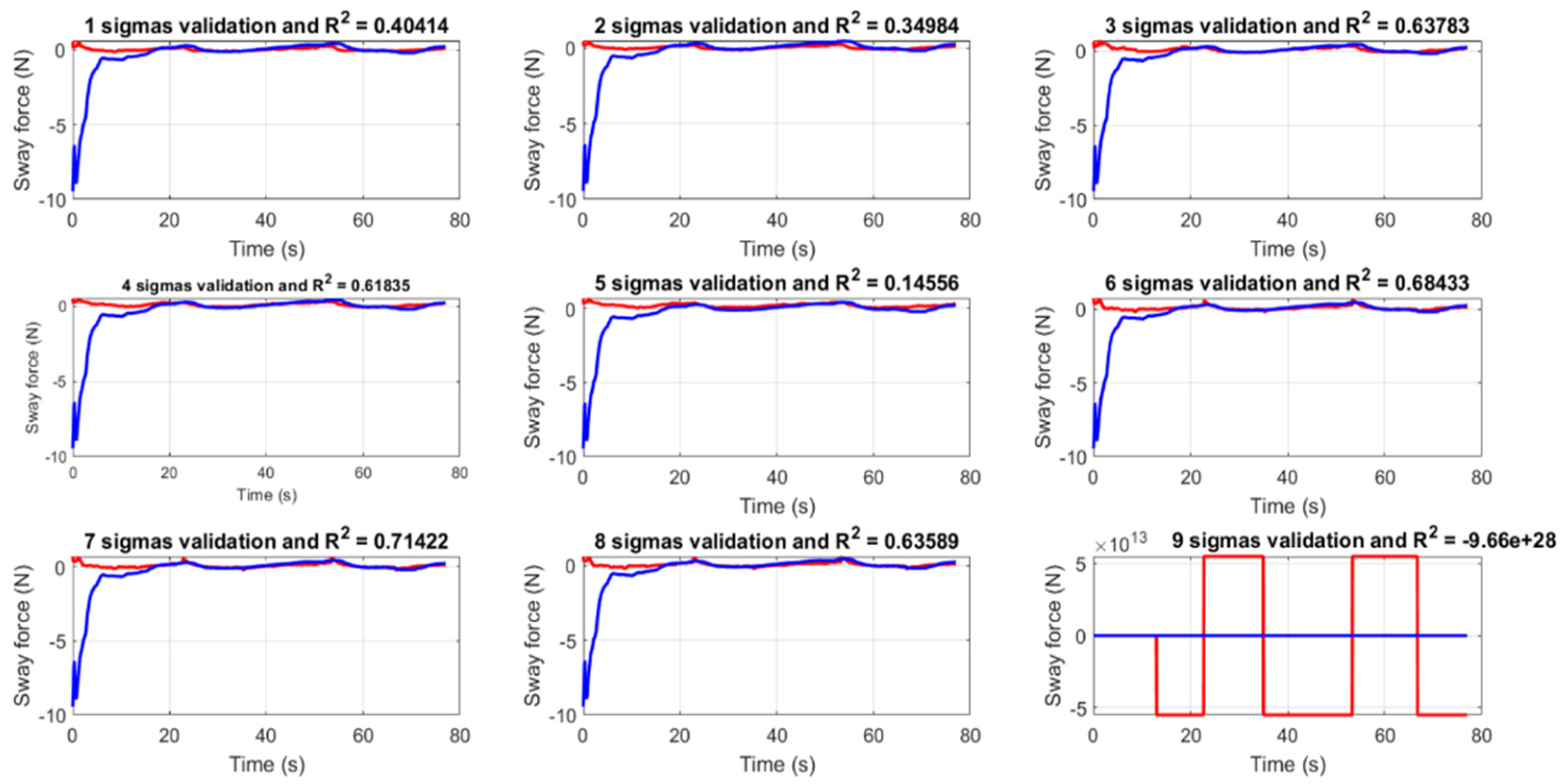
Then, the validation was performed by applying the adjustment coefficient results from the identification to the performed 20°–20° zigzag manoeuvre in the free-running tests. The measured forces and moments were plotted together and compared.

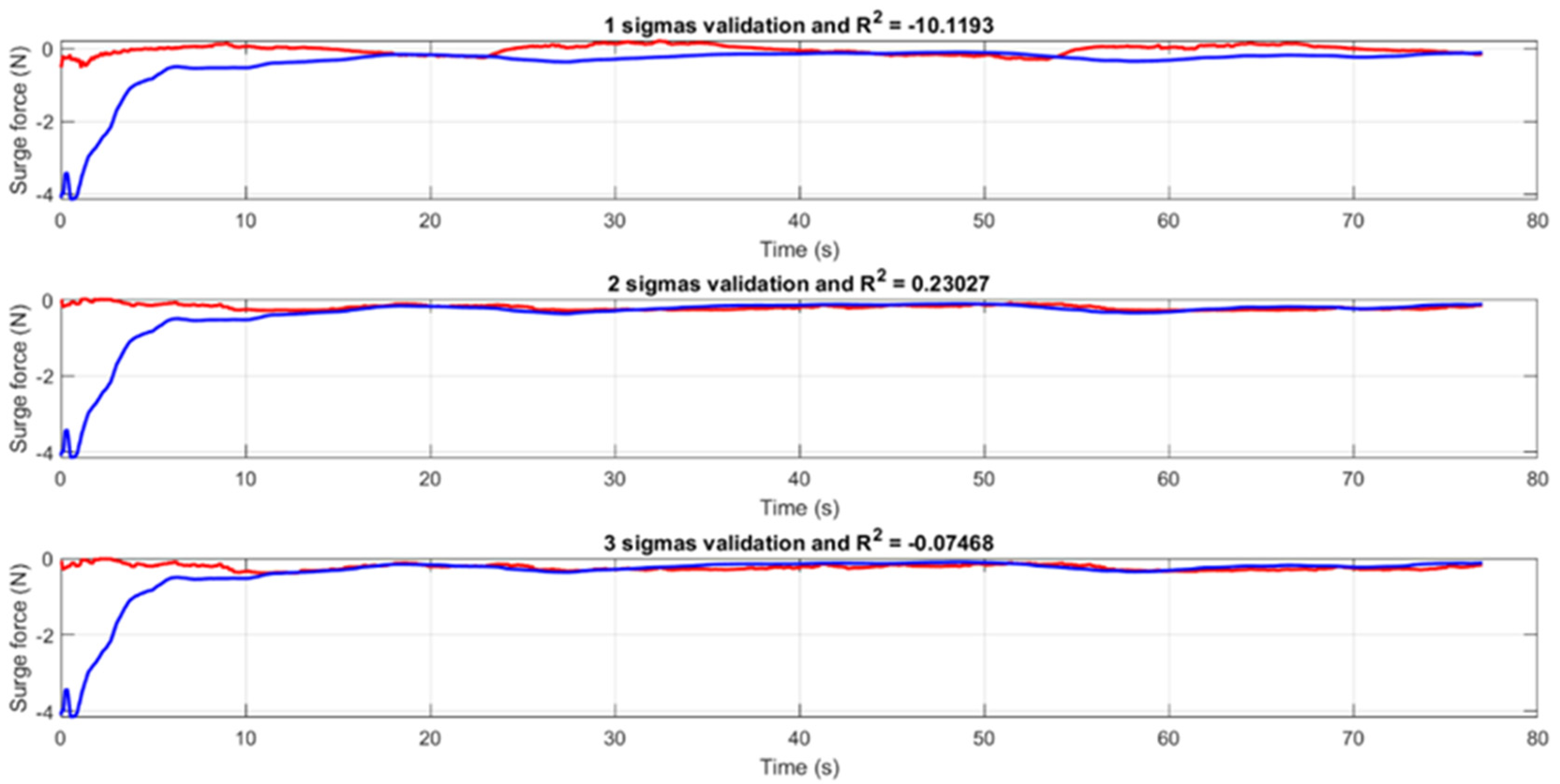
As in the simulation results, the validation for the surge motion confirmed the identification results, as two singular values gave better validation results (Figure 12) with the best coefficient of determination.

For both for sway and yaw manoeuvres, the validation had good values (Figure 13 and Figure 14). For sway, there were more good fits with the validation when compared with the identification. The results for k = 3, 4, 6, 7, 8 validated well. However, the uncertainties for four and eight singular values were very large in the identification and the coefficient of determination was quite low for three singular values in the identification as well. Thus, the validations for six and seven singular values were the ones in concordance with the identification of coefficients for the free-running tests’ data. The same occurred with the yaw motion, with good validation for six and seven singular values. The latter had large uncertainties in the identification, making it not acceptable for the results of coefficients.

The fact that there were some validations that were good for a number of singular values that provides bad results in identification prove that some parameter drift can happen, and that even if the manoeuvres are well predicted (good validation) the values are far from good (bad identification). Parameter drift can also be linked to multicollinearity and environmental surroundings, as the validation from nine singular values had huge coefficients of determination in both sway and yaw motion, with no fitting between the measured and estimated forces and moments.

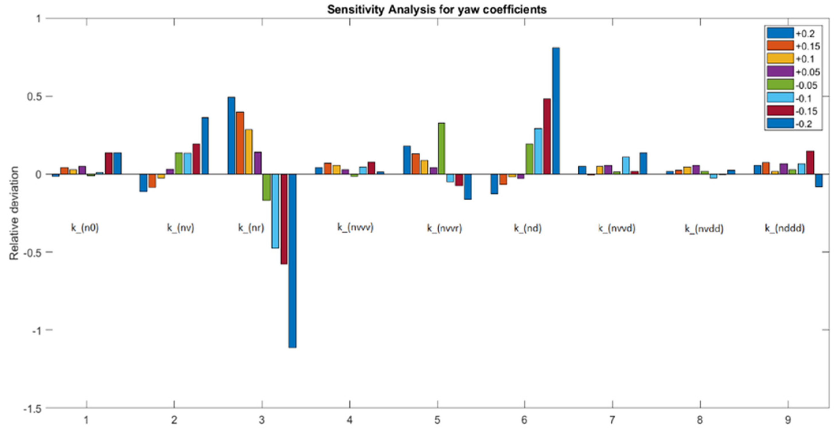
5.3. Sensitivity Analysis

To study the sensitivity analysis, the 20°–20° zigzag manoeuvre from the simulation was chosen, having no interference from environmental elements. The analysis was performed for all the adjustment coefficients (21 in total), varying them individually with the following percentages: +20%, +15%, +10%, +5%, −5%, −10%, −15%, and −20% (eight variations per each coefficient). The analysed parameter for the sensitivity analysis was the overshoot angle. This is the most common parameter to analyse when using zigzag manoeuvres [36]. In this fashion, all the overshoot angles from all the variations of all the coefficients were compared with the original ones (unitary coefficients). The relative deviation (Equation (25)), concerning the overshoot angle, was then computed and plotted (Figure 15, Figure 16 and Figure 17).

$$\Delta E_i=\frac{E_i}{\sum E_i}$$

(25)

where $\Delta E_i$ is the relative deviation, $E_i$ is the deviation from the original overshoot angle regarding the variation of the coefficient being analysed, and $\mathsf{\Sigma }{E}_i$ is the sum of all the deviations from the original overshoot angle for the analysed coefficient.

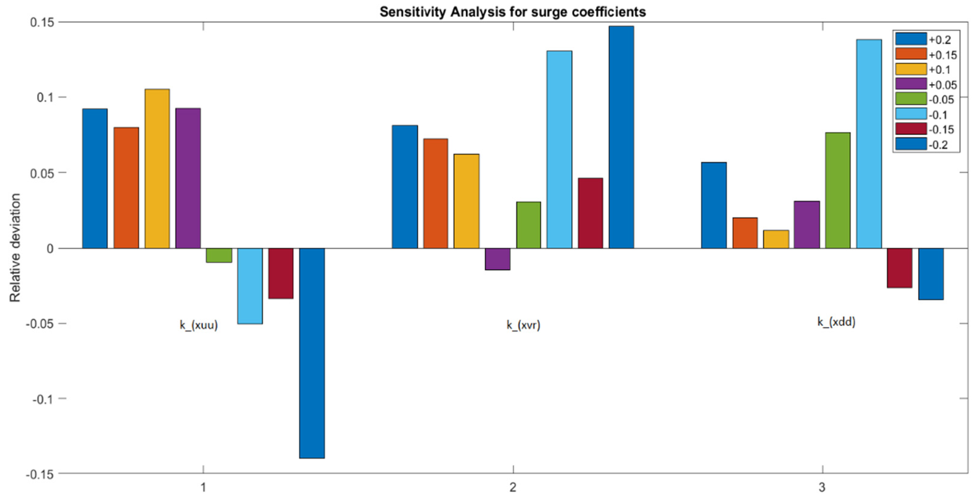
For surge motion coefficients, all three coefficients are important (Figure 15). However, there are two which stood out: $k_{xuu}$ and $k_{xvr}$. The first one had a bigger relative deviation when the variations were positive, and the second one when the variations were negative. The results match with the ones from the identification and validation of the adjustment coefficients, which for surge had better results with two singular values.

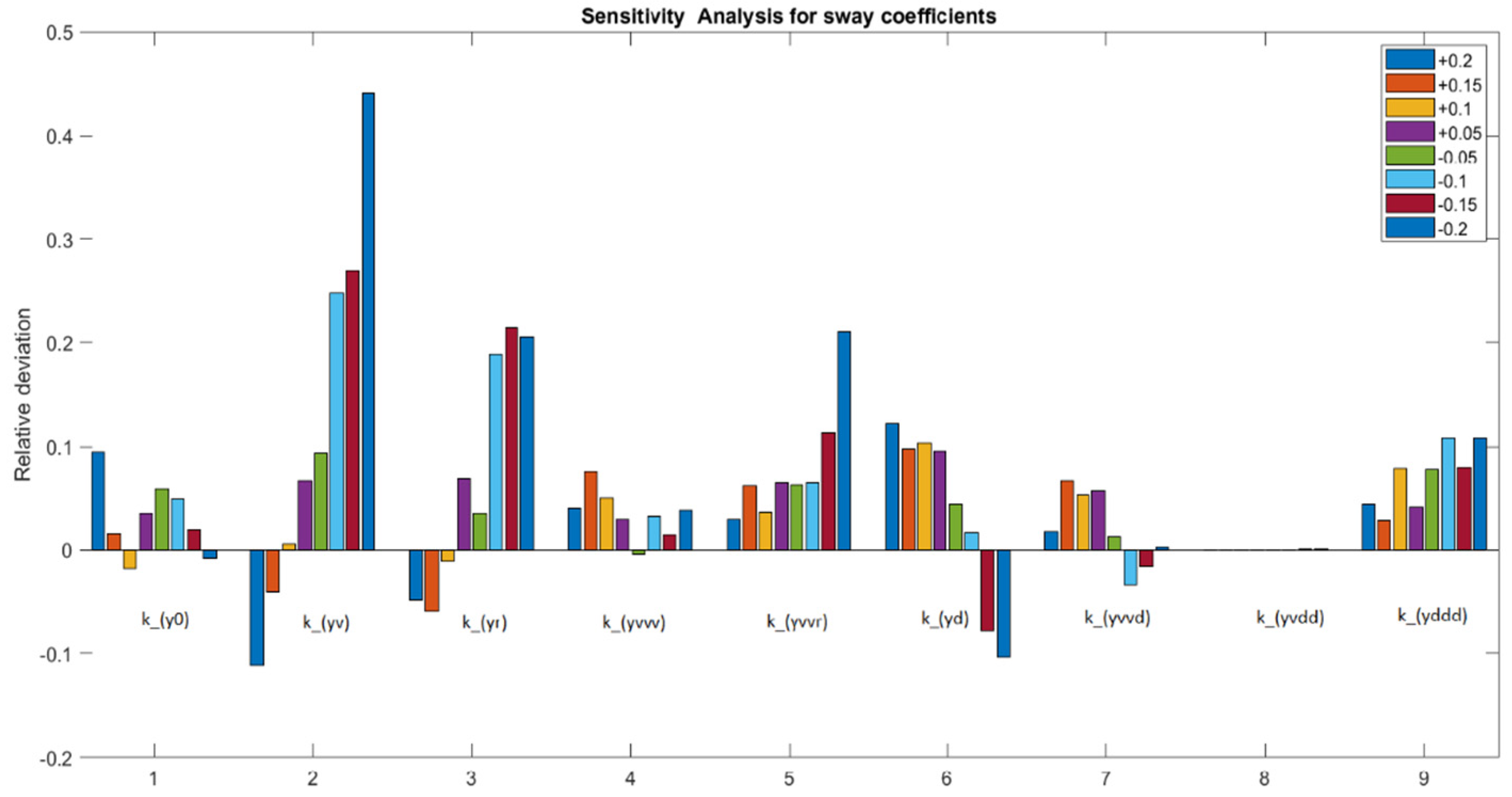
The sway coefficients were the most expressive ones (Figure 16), as some were influential (such as $k_{yv}$ and $k_{yr}$) and others, such as $k_{yv\delta \delta }$, had in influence at all. There were five coefficients ($k_{yv}$, $k_{yr}$, $k_{yd}$, $k_{yvvr}$, and $k_{y\delta \delta \delta }$) which had a larger relative deviation, meaning a large influence on the manoeuvring model and the results. The other remaining three were also important. However, they were not as relevant for all the deviations. Therefore, they are not as crucial for all ranges of variations that can occur when computing the adjustment coefficients and the final mathematical manoeuvring model.

Finally, regarding the yaw coefficients, the linear and the rudder coefficients $k_{nv}$, $k_{nr}$, and $k_{nd}$ were the most important ones. The relative deviations were much larger considering the yaw coefficients than in the previous two motions. In the previous motions, the maximum sensitivity was below 15% for surge and 50% for sway. However, in the yaw motion, there was one variation that went beyond 100%, and others that were between 50% and 100%. Additionally, it had more coefficients with less influence when compared with sway. The coefficients $k_{n0}$, $k_{nvvv}$, $k_{nvvd}$, $k_{nvdd}$, and $k_{nddd}$ had smaller relative deviations regarding the yaw coefficients, even if they were in the range of the higher ones in the surge and sway motions.

Interestingly, regarding the motion, almost no coefficient behaved in the same way regarding the variation from unitary values. Only $k_{y\delta \delta \delta }$ had a consistent positive relative deviation with all eight variations. Additionally, the sensitivity analysis also corroborated the identification and validation of the coefficients. This once again proves that not all the coefficients are necessary to predict a manoeuvre and that can be used as an aid to the least squares method combined with the truncated singular value decomposition to have a better final response to the best estimate of the adjustment coefficients.

6. Conclusions

In this study, an estimation of the adjustment coefficients was performed using a least squares method combined with the truncated singular value decomposition. The addition of the truncated singular value decomposition allowed for a better estimation of the coefficients as the parameter uncertainty was handled better. This was verified both for data from simulation and data from free-running tests. As expected, due to the existence of environmental disturbances, the results from the tests’ data were not as good as those from the simulation. Nonetheless, they were consistent with the fact that fewer coefficients were better to predict a manoeuvre, having less problems with uncertainties and fit between measured and estimated forces and moments. Thus, the problems of multicollinearity and parameter drift (present in the validation of coefficients from the tests’ data) were managed and satisfactory results were achieved.

The addition of sensitivity analysis allowed for a greater look at the influence of each coefficient in the manoeuvres. Once again, as anticipated in the literature, not all the coefficients had the same importance for the manoeuvres. This was corroborated with the sensitivity analysis, which helped predict the most crucial coefficients for each motion. Moreover, the least squares method combined with the truncated singular value decomposition can be improved by introducing the relative weight factors in the future if the results are linked with sensitivity analysis.

References

1. Sutulo, S.; Guedes Soares, C. Mathematical models for simulation of manoeuvring performance of ships. In Marine Technology and Engineering; Guedes Soares, C., Garbatov, Y., Fonseca, N., Teixeira, A.P., Eds.; Taylor & Francis Group: London, UK, 2011; pp. 661–698. [Google Scholar]
2. Abkowitz, M.A. Measurements of hydrodynamic characteristics from ship maneuvering trials by system identification. Trans. SNAME 1980, 88, 283–318. [Google Scholar]
3. Källström, C.G.; Åström, K.J. Experiences of System Identification Applied to Ship Steering. Automatica 1981, 17, 187–198. [Google Scholar] [CrossRef]
4. Skjetne, R.; Smogeli, Ø.N.; Fossen, T.I. A nonlinear ship manoeuvring model: Identification and adaptive control with experiments for a model ship. Model. Identif. Control 2004, 25, 3–27. [Google Scholar] [CrossRef] [Green Version]
5. Luo, W.L.; Zou, Z.J. Parametric Identification of Ship Maneuvering Models by Using Support Vector Machines. J. Ship Res. 2009, 53, 19–30. [Google Scholar] [CrossRef]
6. Araki, M.; Sadat-Hosseini, H.; Sanada, Y.; Tanimoto, K.; Umeda, N.; Stern, F. Estimating maneuvering coefficients using system identification methods with experimental, system-based, and CFD free-running trila data. Ocean Eng. 2012, 51, 63–84. [Google Scholar] [CrossRef] [Green Version]
7. Zhu, M.; Hahn, A.; Wen, Y.-Q.; Bolles, A. Identification-based simplified model of large container ships using support vector machines and artificial bee colony algorithm. Appl. Ocean Res. 2017, 68, 249–261. [Google Scholar] [CrossRef]
8. Wang, Z.; Xu, H.; Xia, L.; Zou, Z.; Guedes Soares, C. Kernel-based support vector regression for nonparametric modeling of ship maneuvering motion. Ocean Eng. 2020, 216, 107994. [Google Scholar] [CrossRef]
9. Moreira, L.; Guedes Soares, C. Dynamic Model of Manoeuvrability using Recursive Neural Networks. Ocean Eng. 2003, 30, 1669–1697. [Google Scholar] [CrossRef]
10. Luo, W.L.; Moreira, L.; Guedes Soares, C. Manoeuvring Simulation of Catamaran by Using Implicit Models Based on Support Vector Machines. Ocean Eng. 2014, 82, 150–159. [Google Scholar] [CrossRef]
11. Sutulo, S.; Moreira, L.; Guedes Soares, C. Mathematical Models for Ship Path Prediction in Manoeuvring Simulation Systems. Ocean Eng. 2002, 29, 1–19. [Google Scholar] [CrossRef]
12. Xu, H.T.; Oliveira, P.; Guedes Soares, C. L1 adaptive backstepping control for path-following of underactuated marine surface ship. Eur. J. Control 2021, 58, 357–372. [Google Scholar] [CrossRef]
13. Guedes Soares, C.; Sutulo, S.; Francisco, R.A.; Santos, F.M.; Moreira, L. Full-Scale Measurements of the Manoeuvring Capabilities of a Catamaran. In Proceedings of the RINA International Conference “Hydrodynamics of High-Speed Craft”, London, UK, 24–25 November 1999; pp. 1–12. [Google Scholar]
14. Guedes Soares, C.; Francisco, R.A.; Moreira, L.; Laranjinha, M. Full-Scale Measurements of the Manoeuvering Capabilities of Fast Patrol Vessels, Argos Class. Mar. Technol. SNAME News 2004, 41, 7–16. [Google Scholar] [CrossRef]
15. Delefortrie, G.; Eloot, K.; Lataire, E.; Van Hoydonck, W.; Vantorre, M. Captive model tests based 6 DOF shallow water manoeuvring model. In Proceedings of the 4th MASHCON-International Conference on Ship Manoeuvring in Shallow and Confined Water with Special Focus on Ship Bottom Interaction, Hamburg, Germany, 23–25 May 2016; pp. 273–286. [Google Scholar]
16. Sutulo, S.; Guedes Soares, C. Development of a Multifactor Regression Model of Ship Maneuvering Forces Based on Optimized Captive-Model Tests. J. Ship Res. 2006, 50, 311–333. [Google Scholar] [CrossRef]
17. Hochbaum, A.; Stern, F.; Agdrup, K.; Broglia, R.; Kim, S.; Perdon, P.; Quadvlieg, F.; Yasukawa, H.; Zou, Z. The manoeuvring committee-final report and recommendations to the 25th ITTC. In Proceedings of the 25th International Towing Tank Conference, Fukuoka, Japan, 14–20 September 2008; pp. 143–208. [Google Scholar]
18. Viviani, M.; Bonvino, C.P.; Depascale, R.; Conti, F.; Soave, M. Identification of hydrodynamic coefficient from standard manoeuvres for a series of twin-screw ships. In Proceedings of the 2nd International Conference on Marine Research and Transportation, Naples, Italy, 28–30 June 2007; pp. 99–108. [Google Scholar]
19. Xu, H.; Guedes Soares, C. Hydrodynamic coefficient estimation for ship manoeuvring in shallow water using an optimal truncated ls-svm. Ocean Eng. 2019, 191, 106488. [Google Scholar] [CrossRef]
20. Xu, H.; Guedes Soares, C. Manoeuvring modelling of a containership in shallow water based on optimal truncated nonlinear kernel-based least square support vector machine and quantum inspired evolutionary algorithm. Ocean Eng. 2020, 195, 106676. [Google Scholar] [CrossRef]
21. Xu, H.; Hassani, V.; Guedes Soares, C. Comparing generic and vectorial nonlinear manoeuvring models and parameter estimation using optimal truncated least square support vector machine. Appl. Ocean Res. 2020, 97, 102061. [Google Scholar] [CrossRef]
22. Xu, H.; Hinostroza, M.; Guedes Soares, C. Estimation of hydrodynamic coefficients of a nonlinear manoeuvring mathematical model with free-running ship model tests. Int. J. Marit. Eng. 2018, 160, A213–A225. [Google Scholar]
23. Farrar, D.E.; Glauber, R.R. Multicollinearity in regression analysis: The problem revisited. Rev. Econ. Stat. 1967, 49, 92–107. [Google Scholar] [CrossRef]
24. Wang, X.-G.; Zou, Z.-J.; Xu, F.; Ren, R.-Y. Sensitivity analysis and parametric identification for ship manoeuvring in 4 degrees of freedom. J. Mar. Sci. Technol. 2014, 19, 394–405. [Google Scholar] [CrossRef]
25. Haddara, M.R.; Wang, Y. Parametric identification of manoeuvring models for ships. Int. Shipbuild. Prog. 1999, 46, 5–27. [Google Scholar]
26. Zhang, X.-G.; Zou, Z.-J. Identification of Abkowitz model for ship manoeuvring motion using ″ε-support vector regression. J. Hydrodyn. 2011, 23, 353–360. [Google Scholar] [CrossRef]
27. Le, M.-D.; Kose, K. Estimation of ship hydrodynamic coefficients at low speed range and application to control ships. J. Jpn. Inst. Navig. 2000, 103, 33–39. [Google Scholar] [CrossRef]
28. Xu, H.; Hassani, V.; Guedes Soares, C. Uncertainty analysis of the hydrodynamic coefficients estimation of a nonlinear manoeuvring model based on planar motion mechanism tests. Ocean Eng. 2019, 173, 450–459. [Google Scholar] [CrossRef]
29. Xu, H.; Hassani, V.; Guedes Soares, C. Truncated least square support vector machine for parameter estimation of a nonlinear manoeuvring model based on PMM tests. Appl. Ocean. Res. 2020, 97, 102076. [Google Scholar] [CrossRef]
30. Sutulo, S.; Guedes Soares, C. An algorithm for offline identification of ship manoeuvring mathematical models from free-running tests. Ocean Eng. 2014, 79, 10–25. [Google Scholar] [CrossRef]
31. Luo, W.; Guedes Soares, C.; Zou, Z. Parameter identification of ship maneuvering model based on support vector machines and particle swarm optimization. J. Offshore Mech. Arct. Eng. 2016, 138, 031101. [Google Scholar] [CrossRef]
32. Rajesh, G.; Bhattacharyya, S.K. System identification for nonlinear maneuvering of large tankers using artificial neural network. Appl. Ocean. Res. 2008, 30, 256–263. [Google Scholar] [CrossRef]
33. Ferrari, V.; Perera, L.P.; Santos, F.P.; Hinostroza, M.A.; Sutulo, S.; Guedes Soares, C. Initial experimental tests of a research-oriented self-running ship model. In Maritime Technology and Engineering; Guedes Soares, C., Santos, T.A., Eds.; Taylor & Francis Group: London, UK, 2015; pp. 913–918. [Google Scholar]
34. Perera, L.P.; Ferrari, V.; Santos, F.P.; Hinostroza, M.A.; Guedes Soares, C. Experimental Evaluations on Ship Autonomous Navigation and Collision Avoidance by Intelligent Guidance. IEEE J. Ocean Eng. 2015, 40, 374–387. [Google Scholar] [CrossRef]
35. Hansen, P.C. The truncated svd as a method for regularization. BIT Numer. Math. 1987, 27, 534–553. [Google Scholar] [CrossRef]
36. Kim, D.; Kim, S.-H.; Kim, S.-J.; Paik, K.-J. A study on the sensitivity analysis of the hydrodynamic derivatives on the maneuverability of KVLCC2 in shallow water. Brodogradnja 2017, 68, 1–22. [Google Scholar] [CrossRef] [Green Version]
Figure 1. The free-running ship model during the manoeuvring tests.
Jmse 09 01302 g001
Figure 2. Sensors and actuators installed on the ship model.
Jmse 09 01302 g002
Figure 3. Measured surge force (blue curves) vs. estimated surge forces (red curves) for 25° turning manoeuvre.
Jmse 09 01302 g003
Figure 4. Measured (blue curves) vs. estimated sway forces (red curves) for 25° turning manoeuvre.
Jmse 09 01302 g004
Figure 5. Measured (blue curves) vs. estimated yaw moment (red curves) for 25° turning manoeuvre.
Jmse 09 01302 g005
Figure 6. Results from the validation for surge motion with a 20°−20° zigzag manoeuvre.
Jmse 09 01302 g006
Figure 7. Results from the validation for sway motion with a 20°−20° zigzag manoeuvre.
Jmse 09 01302 g007
Figure 8. Results from the validation for yaw motion with a 20°−20° zigzag manoeuvre.
Jmse 09 01302 g008
Figure 9. Measured (blue curves) vs. estimated surge force (red curves) for the tests’ data from the 30°−30° zigzag manoeuvre.
Jmse 09 01302 g009
Figure 10. Measured (blue curves) vs. estimated sway force (red curves) for the tests’ data from the 30°−30° zigzag manoeuvre.
Jmse 09 01302 g010
Figure 11. Measured yaw moment (blue curves) vs. estimated yaw moment (red curves) for the test’s data from the 30°−30° zigzag manoeuvre.
Jmse 09 01302 g011
Figure 12. Results from the validation for surge motion with 20°−20° zigzag manoeuvre tests’ data.
Jmse 09 01302 g012
Figure 13. Results from the validation for sway motion with a 20°–20° zigzag manoeuvre tests’ data.
Jmse 09 01302 g013
Figure 14. Results from the validation for yaw motion with 20°–20° zigzag manoeuvre tests’ data.
Jmse 09 01302 g014
Figure 15. Sensitivity analysis for surge coefficients.
Jmse 09 01302 g015
Figure 16. Sensitivity analysis for sway coefficients.
Jmse 09 01302 g016
Figure 17. Sensitivity analysis for yaw coefficients.
Jmse 09 01302 g017