Parasitic Capillary Waves on Small-Amplitude Gravity Waves with a Linear Shear Current

Abstract

This paper describes a numerical investigation of ripples generated on the front face of deep-water gravity waves progressing on a vertically sheared current with the linearly changing horizontal velocity distribution, namely parasitic capillary waves with a linear shear current. A method of fully nonlinear computation using conformal mapping of the flow domain onto the lower half of a complex plane enables us to obtain highly accurate solutions for this phenomenon with the wide range of parameters. Numerical examples demonstrated that, in the presence of a linear shear current, the curvature of surface of underlying gravity waves depends on the shear strength, the wave energy can be transferred from gravity waves to capillary waves and parasitic capillary waves can be generated even if the wave amplitude is very small. In addition, it is shown that an approximate model valid for small-amplitude gravity waves in a linear shear current can reasonably well reproduce the generation of parasitic capillary waves.

1. Introduction

It is well known that a vertically sheared current affects the nonlinear motion of surface waves progressing on water and plays important roles in the ocean (see reviews by Peregrine [1]). In this work, we focus on its effects on ripples produced on the forward face of progressive gravity waves, which are referred to as “parasitic capillary waves” [2]. The complete understanding of parasitic capillary waves helps us accurately estimate the sea surface elevation from satellite images for remote sensing of ocean surfaces. The generation of such capillary waves is intimately related to the curvature of the water surface of underlying gravity waves as well as the characteristics of the current. Until now, few attempts have been made yet to systematically investigate the interaction between parasitic capillary waves and a vertically sheared current. The aim of this work is to numerically study this nonlinear interaction.

Since Cox’s experiments [3] and Longuet-Higgins’ theoretical work [4], parasitic capillary waves have been studied by various authors [2]. The essential mechanism for the generation of parasitic capillary waves is the nonlinear and unsteady interaction between short capillary waves and long gravity waves in an inviscid flow [5,6], which should be studied via fully nonlinear computations. For the irrotational plane flow, we can formulate this problem within the framework of potential theory and conformally map the unsteady flow domain onto a fixed domain such as a strip of uniform thickness or a unit disk in a complex plane, where the free surface is mapped onto its boundary that remains unchanged in time. Murashige & Choi [7] showed that this unsteady conformal mapping technique, which is referred to as the Unsteady Hodograph Transformation (UHT) method, is suitable for fully nonlinear computations of parasitic capillary waves, and that the UHT method is advantageous in reducing aliasing errors due to spectral approximation.

When a vertically sheared current exists and its horizontal velocity distribution changes linearly, as shown in Figure 1a, the background vorticity is constant and, therefore, any perturbed flows must be irrotational due to conservation of vorticity. Thus we can incorporate this linear shear current into the aforementioned unsteady conformal mapping, or the UHT, technique. In fact, in the presence of a linear shear current, this UHT method has been previously applied to fully nonlinear computation of the two-dimensional unsteady motion of pure gravity periodic waves [8,9] and capillary-gravity solitary waves [10]. It should be noted that the presence of a linear shear current in deep water may be unrealistic in the sense that the fluid velocity tends to infinity with depth. However, our interest is in the short wave motion of parasitic capillary waves, which is limited near the water surface. Therefore, the detailed vorticity distribution far away from the surface might be irrelevant and the linear shear near the surface would be sufficient.

In this work, we numerically examine the effects of the strength of a linear shear current on the generation of parasitic capillary waves using the UHT method. The paper is organized as follows. Formulation of the problem using conformal mapping is presented in Section 2. The method of computation based on a pseudo-spectral method is shown in Section 3. Numerical solutions for the generation of parasitic capillary waves with a linear shear current are summarized in Section 4 and discussed in Section 5. Section 6 concludes this work.

2. Formulation of the Problem

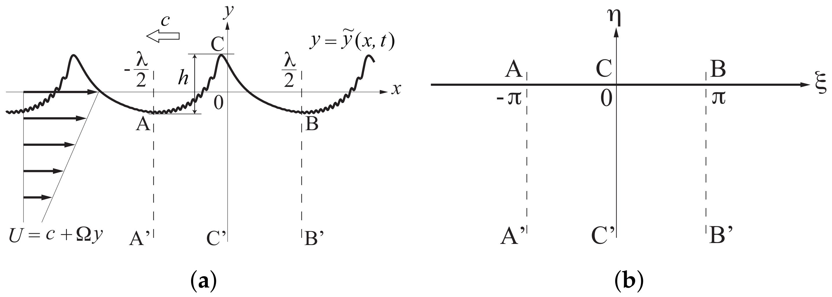
2.1. Formulation in the Physical Plane

Consider the unsteady and periodic motion of deep-water gravity-capillary waves progressing to the left on a linear shear current, as shown in Figure 1a. It is assumed that the fluid motion is two-dimensional in the vertical cross-section (x, y) along the wave propagation direction, and that the fluid is inviscid and incompressible. The origin is placed such that the wave profile $y=\tilde{y}(x,t)$ satisfies the zero mean level condition:

$${\displaystyle {\int }_0^{\lambda }\tilde{y}(x,t)\mathrm{d}x=0.}$$

(1)

It is convenient to formulate the problem in the flow domain over one wavelength $\lambda$ in the frame of reference moving to the left with the wave speed c so that the total horizontal velocity is given by $U=c+\Omega y$, where the shear strength $\Omega$ is constant. Note that waves for $\Omega >0$ and $\Omega <0$ are referred to as upstream and downstream propagating waves, respectively. Then the fluid velocity vector $\mathit{U}$ can be written as

$$\mathit{U}=\left(\begin{array}{c}U\\ V\end{array}\right)=\left(\begin{array}{c}\Omega y\\ 0\end{array}\right)+\left(\begin{array}{c}u\\ v\end{array}\right).$$

(2)

From conservation of vorticity for two-dimensional inviscid flows, the vorticity remains constant if it is initially constant. Thus the perturbed wave motion given by $(u,v)$ is irrotational and can be described by the complex velocity potential f defined by

$${\displaystyle f(z,t)=\varphi (x,y,t)+\mathrm{i}\psi (x,y,t)\mathrm{with}\frac{\partial f}{\partial z}=w=u-\mathrm{i}v,}$$

(3)

where $z=x+\mathrm{i}y$ and $w=u-\mathrm{i}v$ denote the complex coordinate and the complex velocity, respectively, and t is the time. In addition, from the mass conservation law given by $U_x+V_y=0$, one can introduce a streamfunction $\Psi$ defined by

$$U={\Psi }_y\mathrm{and}V=-{\Psi }_x.$$

(4)

From (2) and (3), $\Psi$ is related to $\psi =\mathrm{Im}\left\{f\right\}$ by

$${\displaystyle \Psi =\frac{1}{2}\Omega y^2+\psi .}$$

(5)

With the characteristic speed c and wavelength $\lambda$, all physical variables are non-dimensionalized as follows:

$${\displaystyle z_{*}=kz,t_{*}=ckt,f_{*}=\frac{f}{(c/k)},{\tilde{y}}_{*}=k\tilde{y},h_{*}=kh,}$$

(6)

where $k=2\pi /\lambda$ is the wavenumber and h is the wave crest-to-trough height. Then the following dimensionless parameters appear in the problem:

$${\displaystyle {\Omega }_{*}=\frac{\Omega }{\sqrt{gk}},c_{*}=\frac{c}{\sqrt{g/k}},W_e=\frac{\rho c^2\lambda }{T},\alpha =\frac{h}{\lambda },}$$

(7)

where g is the gravitational acceleration, $W_e$ is the Weber number, $\rho$ is the density of fluid, T is the surface tension, $\alpha$ is the wave steepness, and $c_{*}$ is related to the Froude number $F_{\lambda }$ by

$${\displaystyle F_{\lambda }=\frac{c}{\sqrt{g\lambda }}=\frac{1}{\sqrt{2\pi }}{c}_{*}.}$$

(8)

Henceforth the asterisks for dimensionless variables will be omitted for brevity.

The kinematic and dynamic boundary conditions at the water surface $y=\tilde{y}(x,t)$ are given, respectively, by

$${\tilde{y}}_t+\left({\displaystyle {\varphi }_x+\frac{\Omega }{c}\tilde{y}}\right){\tilde{y}}_x={\varphi }_y\mathrm{at}y=\tilde{y}(x,t),$$

(9)

and

$${\displaystyle {\varphi }_t+\frac{1}{2}({{\varphi }_x}^2+{{\varphi }_y}^2)+\frac{1}{c^2}\tilde{y}+\frac{\Omega }{c}(\tilde{y}{\varphi }_x-\psi )-\frac{2\pi }{W_e}\frac{{\tilde{y}}_{xx}}{{(1+{{\tilde{y}}_x}^2)}^{3/2}}=B\left(t\right)\mathrm{at}y=\tilde{y}(x,t),}$$

(10)

where an arbitrary function $B\left(t\right)$ can be absorbed into $\varphi$. Also, the bottom boundary condition as $y\to -\infty$ is given by

$${\displaystyle \left(\begin{array}{c}u\\ v\end{array}\right)\to \left(\begin{array}{c}1\\ 0\end{array}\right)\mathrm{or}\frac{\partial f}{\partial z}={\varphi }_x+\mathrm{i}{\psi }_x\to 1\mathrm{as}y\to -\infty .}$$

(11)

2.2. Unsteady Conformal Mapping of the Flow Domain

Similarly to the previous studies [7,8,9], we introduce a new complex plane, the $\zeta$-plane ($\zeta =\xi +\mathrm{i}\eta$) shown in Figure 1b, where the flow domain is conformally mapped onto the lower half $\eta <0$ and the time-varying water surface is always mapped onto the real axis $\eta =0$. In the $\zeta$-plane, we choose $z=z(\zeta ,t)$ and $f=f(\zeta ,t)$ as dependent variables. Then, the free surface conditions (9) and (10) are transformed, respectively, to

$${\displaystyle y_t=-x_{\xi }·\frac{1}{J}{\Psi }_{\xi }+y_{\xi }·\mathcal{H}\left[{\displaystyle \frac{1}{J}{\Psi }_{\xi }}\right]\mathrm{at}\eta =0,}$$

(12)

and

$${\displaystyle {\varphi }_t-{\varphi }_{\xi }·\mathcal{H}\left[{\displaystyle \frac{1}{J}{\Psi }_{\xi }}\right]+\frac{1}{2}\frac{1}{J}({{\varphi }_{\xi }}^2-{{\psi }_{\xi }}^2)+\frac{1}{c^2}y+\frac{\Omega }{c}\left({\displaystyle \frac{1}{J}{\varphi }_{\xi }y{x}_{\xi }-\psi }\right)-\frac{2\pi }{W_e}\frac{y_{\xi \xi }{x}_{\xi }-x_{\xi \xi }{y}_{\xi }}{J^{3/2}}=B\left(t\right)\mathrm{at}\eta =0,}$$

(13)

where

$${\displaystyle {\Psi }_{\xi }={\psi }_{\xi }+\frac{\Omega }{c}y{y}_{\xi }\mathrm{and}J={x_{\xi }}^2+{y_{\xi }}^2.}$$

(14)

Here the Hilbert transform $\mathcal{H}\left[\mathsf{\Phi }\right(\xi \left)\right]$ of a real valued function $\mathsf{\Phi }\left(\xi \right)$ defined by

$${\displaystyle \mathcal{H}\left[\mathsf{\Phi }\left(\xi \right)\right]:=\frac{1}{\pi }\mathrm{P}.\mathrm{V}.{\int }_{-\infty }^{\infty }\frac{\mathsf{\Phi }\left({\xi }^{\prime }\right)}{{\xi }^{\prime }-\xi }\mathrm{d}{\xi }^{\prime },}$$

(15)

where $\mathrm{P}.\mathrm{V}.$ denotes Cauchy’s principal value. The bottom condition (11) is satisfied with

$$z\to \zeta \mathrm{and}f\to \zeta \mathrm{as}\eta \to -\infty .$$

(16)

We can numerically update the dependent variables y and $\varphi$ with respect to time t using (12) and (13). Note that, at the water surface $\eta =0$, x and $\psi$ are related to y and $\varphi$ by

$$x_{\xi }=1-\mathcal{H}\left[y_{\xi }\right]\mathrm{and}{\psi }_{\xi }=\mathcal{H}[{\varphi }_{\xi }-1]\mathrm{at}\eta =0.$$

(17)

The excess kinetic energy $E_{\mathrm{K}}\left(t\right)$, potential energy $E_{\mathrm{P}}\left(t\right)$ and surface energy $E_{\mathrm{S}}\left(t\right)$ due to the presence of waves can be obtained as

$$\left.\begin{array}{ccc}{E}_{\mathrm{K}}\left(t\right)& =& {\displaystyle \frac{1}{2}\frac{c^2}{{\left(2\pi \right)}^3}\left\{{\displaystyle {\int }_{-\pi }^{\pi }(\psi -y)({\varphi }_{\xi }-x_{\xi })\mathrm{d}\xi +\frac{\Omega }{c}{\int }_{-\pi }^{\pi }({\varphi }_{\xi }-x_{\xi })y^2\mathrm{d}\xi +\frac{1}{3}{\left({\displaystyle \frac{\Omega }{c}}\right)}^2{\int }_{-\pi }^{\pi }{y}^3{x}_{\xi }\mathrm{d}\xi }\right\}}\hfill \\ E_{\mathrm{P}}\left(t\right)& =& {\displaystyle \frac{1}{2}\frac{1}{{\left(2\pi \right)}^3}{\int }_{-\pi }^{\pi }{y}^2{x}_{\xi }\mathrm{d}\xi }\hfill \\ E_{\mathrm{S}}\left(t\right)& =& {\displaystyle \frac{1}{{\left(2\pi \right)}^2}\frac{c^2}{W_e}{\int }_{-\pi }^{\pi }\left(\sqrt{{x_{\xi }}^2+{y_{\xi }}^2}-1\right)\mathrm{d}\xi }\hfill \end{array}\right\},$$

(18)

where each integral is taken along the water surface $-\pi \le \xi \le \pi$ and $\eta =0$ over one period, and each energy is non-dimensionalized by $\rho g{\lambda }^3$.

3. The Method of Computation

Following the previous work [7] (§5.2), we adopt a pseudo-spectral method to solve (12) and (13) for the two unknown variables $y=y(\xi ,t)$ and $\varphi =\varphi (\xi ,t)$ at the water surface $\eta =0$. First, from the analyticity of z and f and the bottom boundary condition (16), $y=y(\xi ,t)$ and $\varphi =\varphi (\xi ,t)$ can be expanded and approximated, respectively, by the following truncated Fourier series

$${\displaystyle y(\xi ,t)\simeq \sum _{k=0}^{N/2}\{b_k\left(t\right)cosk\xi -a_k\left(t\right)sink\xi \},}$$

(19)

and

$${\displaystyle \varphi (\xi ,t)\simeq \xi +\sum _{k=0}^{N/2}\{c_k\left(t\right)cosk\xi +d_k\left(t\right)sink\xi \},}$$

(20)

where $a_k\left(t\right)$, $b_k\left(t\right)$, $c_k\left(t\right)$, and $d_k\left(t\right)$ are all real. For numerical computation, $\xi \in [-\pi ,\pi ]$ is discretized with an equal interval as

$${\xi }_j:=-\pi +j·2\pi /N(j=0,1,\cdots ,N).$$

(21)

When N is set to be a power of 2, the real coefficients $a_k\left(t\right)$, $b_k\left(t\right)$, $c_k\left(t\right)$, and $d_k\left(t\right)$ can be numerically determined from $y_j\left(t\right):=y({\xi }_j,t)$ and ${\varphi }_j\left(t\right):=\varphi ({\xi }_j,t)$ ($j=0,1,\cdots ,N$) using the fast Fourier transform (FFT). We can numerically update $y_j\left(t\right)$ and ${\varphi }_j\left(t\right)$ with respect to the time t using the 4th-order Runge-Kutta method for numerical integration of (12) and (13) by setting a suitable value of the time increment $\Delta t$. Note that the Hilbert transform of $cosk\xi$ and $sink\xi$ are given, respectively, by

$$\left.\begin{array}{ccc}\mathcal{H}[cosk\xi ]& =& \hfill -\mathrm{sgn}\left(k\right)sink\xi \\ \mathcal{H}[sink\xi ]& =& \hfill \mathrm{sgn}\left(k\right)cosk\xi \end{array}\right\}\mathrm{with}\mathrm{sgn}\left(k\right):=\left\{\begin{array}{cc}\hfill +1& (k>0)\\ \hfill 0& (k=0)\\ \hfill -1& (k<0)\end{array}\right..$$

(22)

To estimate the accuracy of the computed results, we monitor an error index $E_{\mathrm{error}}\left(t\right)$ based on the energy conservation law, which is defined by

$$E_{\mathrm{error}}\left(t\right):=|E_{\mathrm{T}}\left(t\right)-E_{\mathrm{T}}\left(0\right)|/E_{\mathrm{T}}\left(0\right)\mathrm{with}{E}_{\mathrm{T}}\left(t\right)=E_{\mathrm{K}}\left(t\right)+E_{\mathrm{P}}\left(t\right)+E_{\mathrm{S}}\left(t\right),$$

(23)

where $E_{\mathrm{K}}\left(t\right)$, $E_{\mathrm{p}}\left(t\right)$, and $E_{\mathrm{S}}\left(t\right)$ are given by (18), and $E_{\mathrm{T}}\left(t\right)$ denotes the total energy of waves.

4. Numerical Results

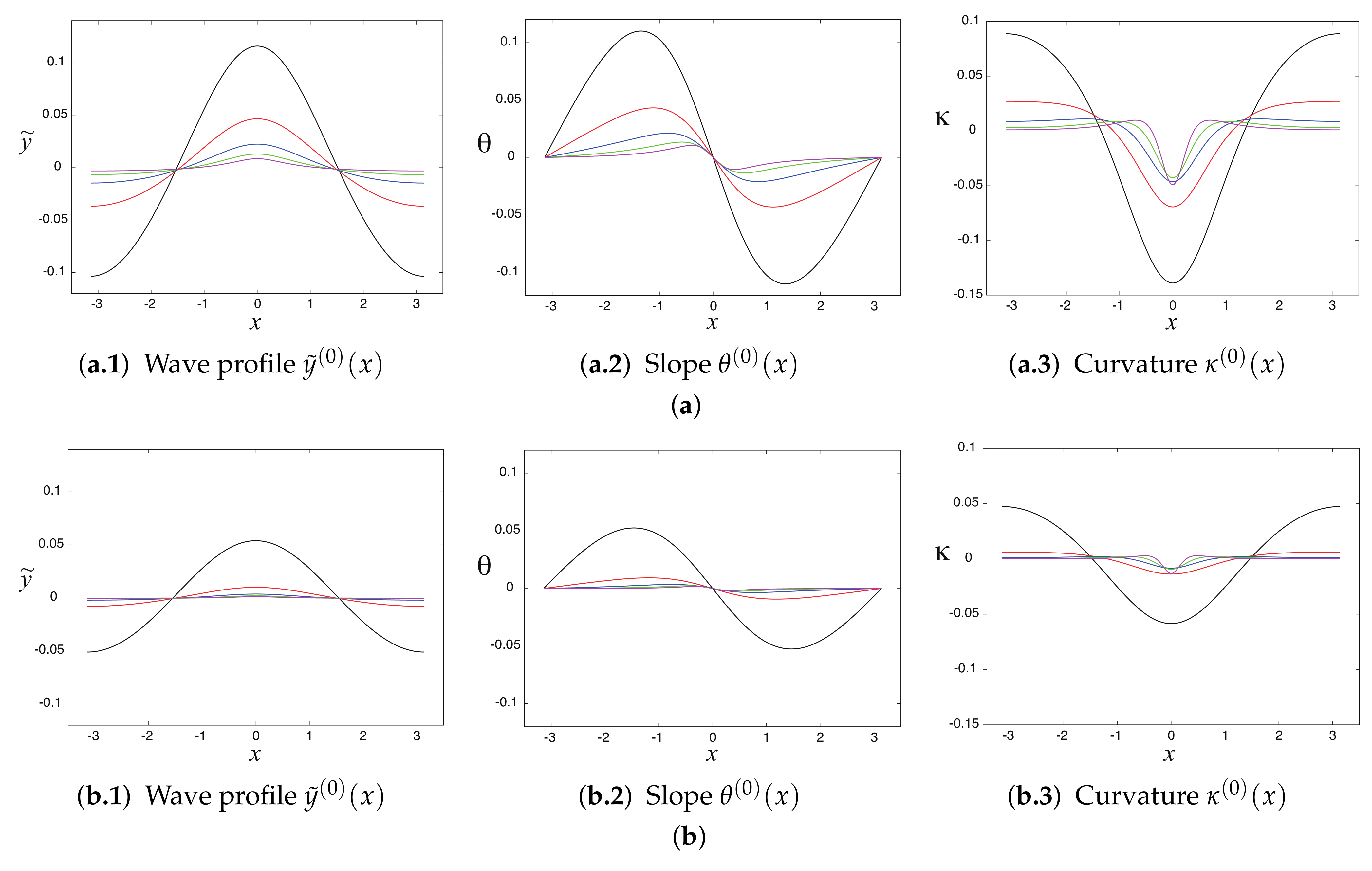
4.1. Initial Values

We assume that symmetric pure gravity waves initially progress in permanent form on a linear shear current. The maximum wave steepness $\alpha$ of the limiting steady waves changes with the shear strength $\Omega$, and thus, similarly to [9], it is convenient to introduce a parameter $\gamma$ defined by

$$\gamma =1-q_{\mathrm{crest}}^{\left(0\right)}/q_{\mathrm{trough}}^{\left(0\right)},$$

(24)

where $q_{\mathrm{crest}}^{\left(0\right)}$ and $q_{\mathrm{trough}}^{\left(0\right)}$ denote the fluid velocity at the wave crest and trough of steady waves, respectively. In this work, we focus on the case of downstream propagating waves, namely $\Omega <0$ because parasitic capillary waves can be easily generated even on small-amplitude gravity waves with a linear shear current for this case, as will be shown in Section 4.2. For $\Omega \le 0$, the parameter $\gamma \in [0,1]$ monotonically increases with the wave steepness $\alpha$ and $\gamma =1$ always corresponds to the limiting wave.

On the assumption of symmetric profile, we can approximate the x and y coordinates of the water surface of $2\pi$-periodic steady waves, $x^{\left(0\right)}\left(\xi \right)$ and $y^{\left(0\right)}\left(\xi \right)$, respectively, by the truncated Fourier series as

$${\displaystyle x^{\left(0\right)}\left(\xi \right)\simeq \xi +\sum _{k=1}^M{b}_k^{\left(0\right)}sink\xi \mathrm{and}{y}^{\left(0\right)}\left(\xi \right)\simeq \sum _{k=0}^M{b}_k^{\left(0\right)}cosk\xi .}$$

(25)

When the parameter $\gamma$ and the shear strength $\Omega$ are given, we may numerically determine the unknown Fourier coefficients $b_k^{\left(0\right)}$ in (25) using Newton’s method such that the free surface conditions (12) and (13) with the zero mean level condition (1) and the condition (24) for $\gamma$ are satisfied. See [9] (§3) for the detailed description of our computational method for these steady waves in the $\zeta$-plane.

Figure 2a,b show the computed results of the wave profile $y={\tilde{y}}^{\left(0\right)}\left(x\right)$, the slope ${\theta }^{\left(0\right)}\left(x\right)$, and the curvature ${\kappa }^{\left(0\right)}\left(x\right)$ of pure gravity steady waves progressing in permanent form on a linear shear current for $\gamma =0.2$ and $0.1$ with some different values of the shear strength $\Omega$, respectively. Here ${\theta }^{\left(0\right)}\left(x\right)$ and ${\kappa }^{\left(0\right)}\left(x\right)$ are given by

$${\displaystyle tan{\theta }^{\left(0\right)}\left(x\right)=\frac{\mathrm{d}{\tilde{y}}^{\left(0\right)}}{\mathrm{d}x}=\frac{y_{\xi }^{\left(0\right)}}{x_{\xi }^{\left(0\right)}}\mathrm{and}{\kappa }^{\left(0\right)}\left(x\right)=\frac{y_{\xi \xi }^{\left(0\right)}{x}_{\xi }^{\left(0\right)}-x_{\xi \xi }^{\left(0\right)}{y}_{\xi }^{\left(0\right)}}{{J^{\left(0\right)}}^{3/2}},}$$

(26)

where $J^{\left(0\right)}={\left(x_{\xi }^{\left(0\right)}\right)}^2+{\left(y_{\xi }^{\left(0\right)}\right)}^2$. The number of Fourier modes in (25) is set to $M=128$, and the computed results using Newton’s method are obtained with an error tolerance smaller than ${10}^{-11}$. It is found that, in the presence of a linear shear current with $\Omega <0$, the curvature ${\kappa }^{\left(0\right)}\left(x\right)$ can be relatively large near the crest $x=0$ even if the wave steepness $\alpha$ is very small such as $\alpha =\mathrm{O}\left({10}^{-3}\right)$ or $\mathrm{O}\left({10}^{-4}\right)$.

Table 1. The wave speed c and the wave steepness $\alpha$ of pure gravity steady waves on a linear shear current in Figure 2. The parameter $\gamma$ is defined by (24) and $\Omega$ is the shear strength. See the definition of dimensionless parameters in (7).

$\mathit{\gamma }$	$\mathsf{\Omega }$	c	$\mathit{\alpha }$
0.2	0.0	1.00604 × 10${}^{+0}$	3.49321 × 10${}^{-2}$
0.2	−1.0	6.22553 × 10${}^{-1}$	1.32682 × 10${}^{-2}$
0.2	−2.0	4.19196 × 10${}^{-1}$	5.90622 × 10${}^{-3}$
0.2	−3.0	3.08239 × 10${}^{-1}$	3.11534 × 10${}^{-3}$
0.2	−4.0	2.41766 × 10${}^{-1}$	1.86715 × 10${}^{-3}$
0.1	0.0	1.00138 × 10${}^{+0}$	1.67068 × 10${}^{-2}$
0.1	−2.0	4.15398 × 10${}^{-1}$	2.85668 × 10${}^{-3}$
0.1	−4.0	2.37640 × 10${}^{-1}$	9.20809 × 10${}^{-4}$
0.1	−6.0	1.64103 × 10${}^{-1}$	4.30888 × 10${}^{-4}$
0.1	−8.0	1.24961 × 10${}^{-1}$	2.45879 × 10${}^{-4}$

summarizes the wave speed c and the wave steepness $\alpha$ of each steady wave solution for given $\gamma$ and $\Omega$ .

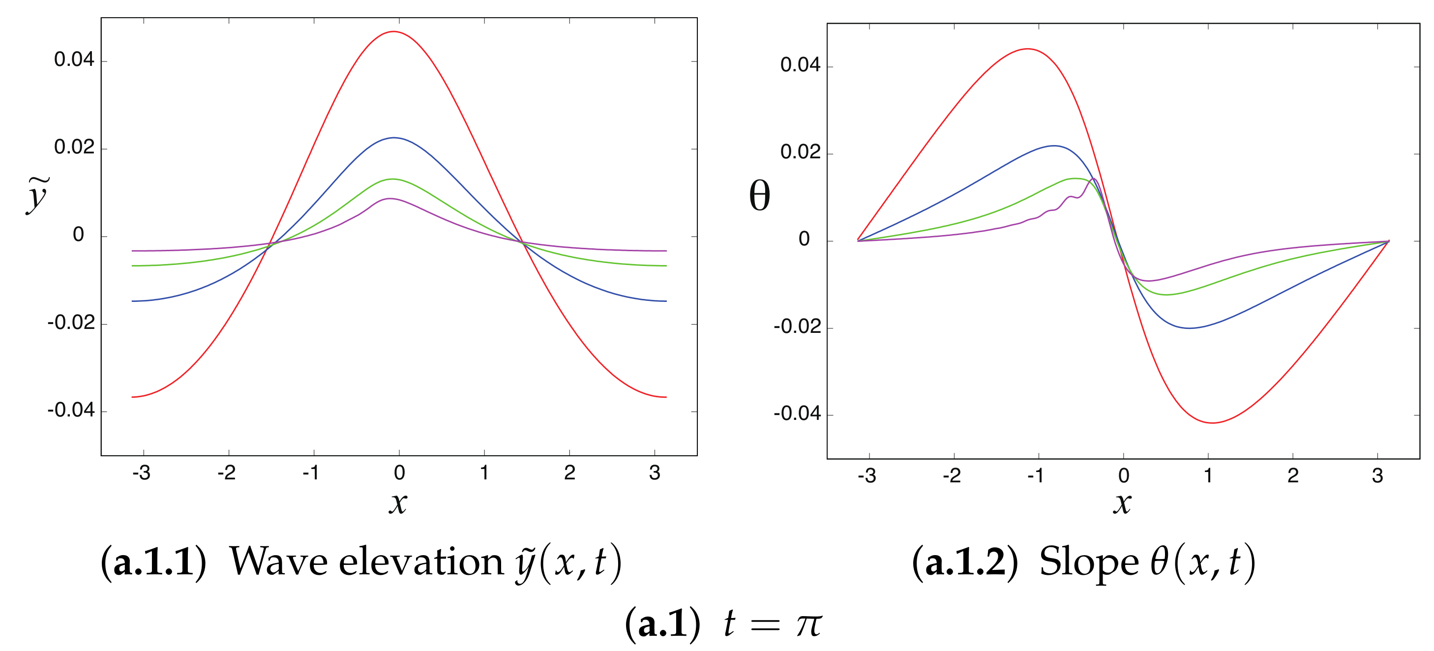
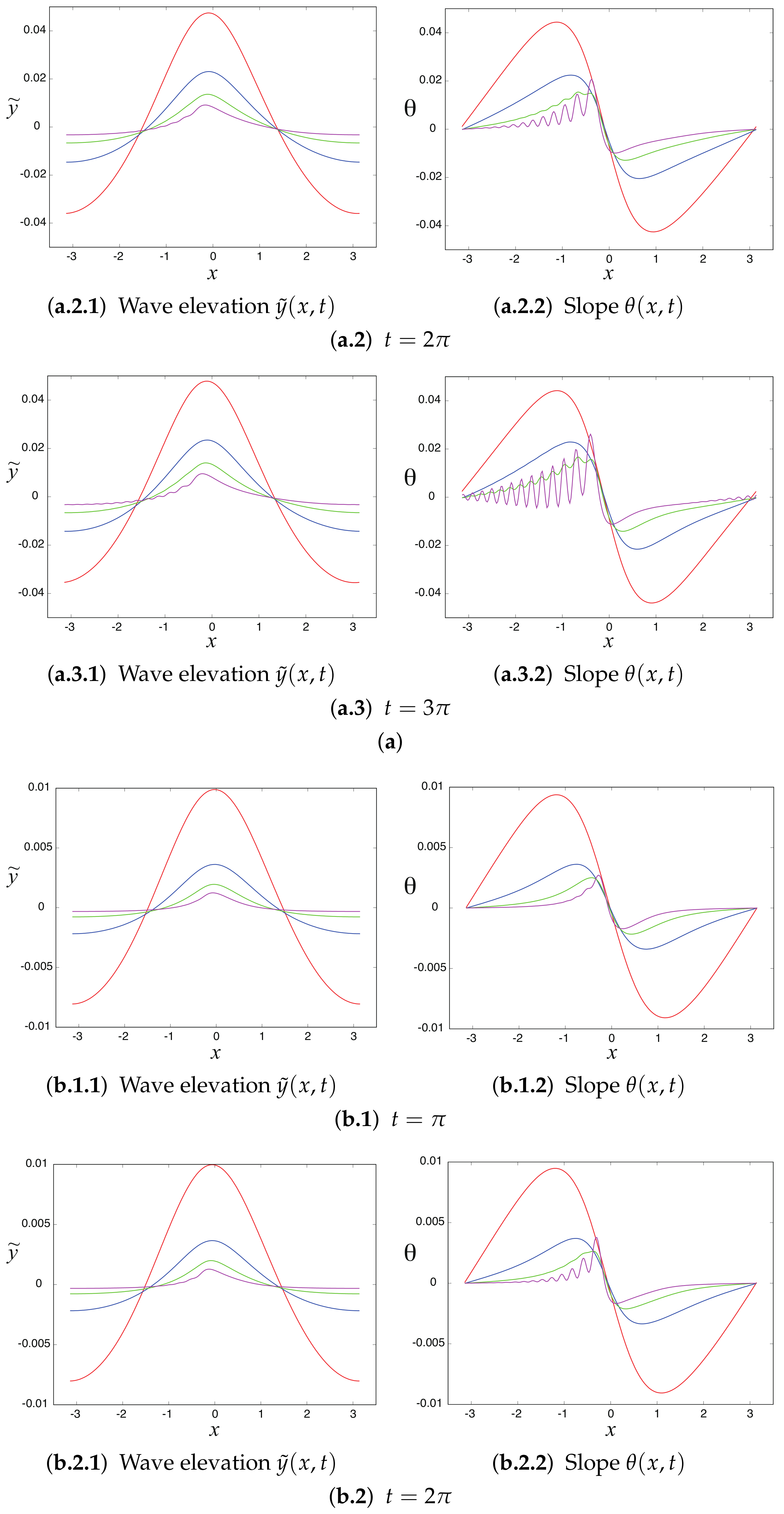
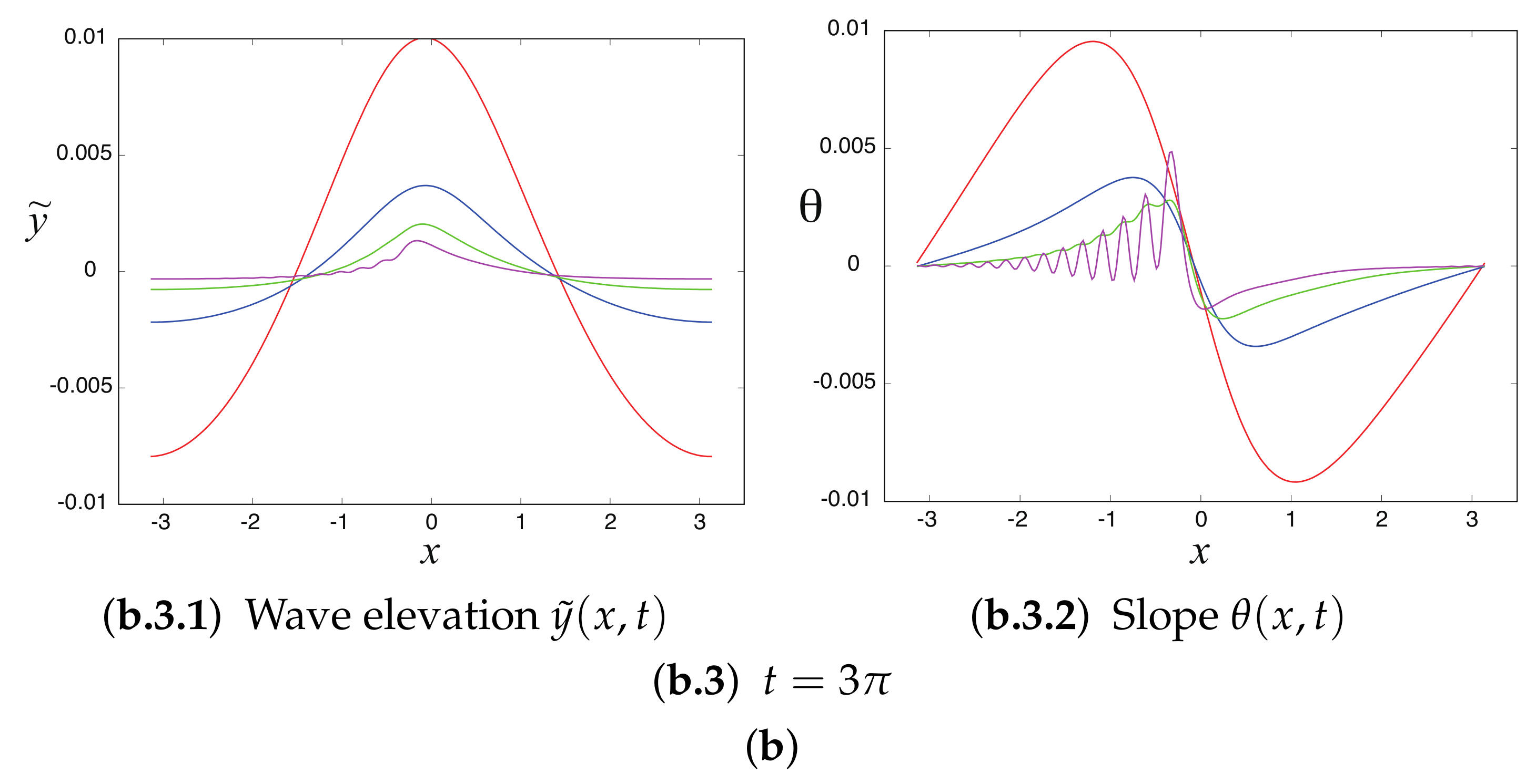
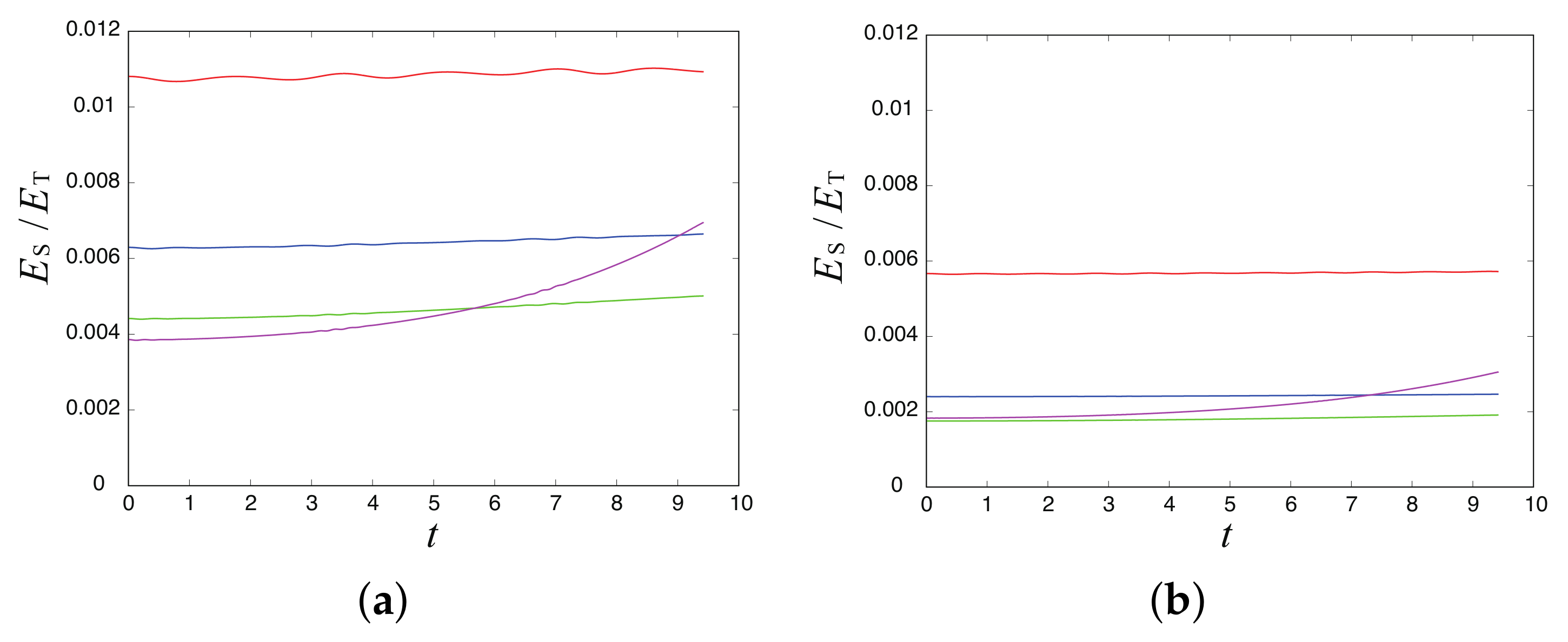
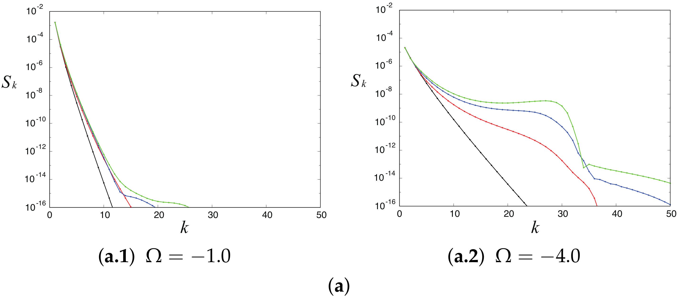
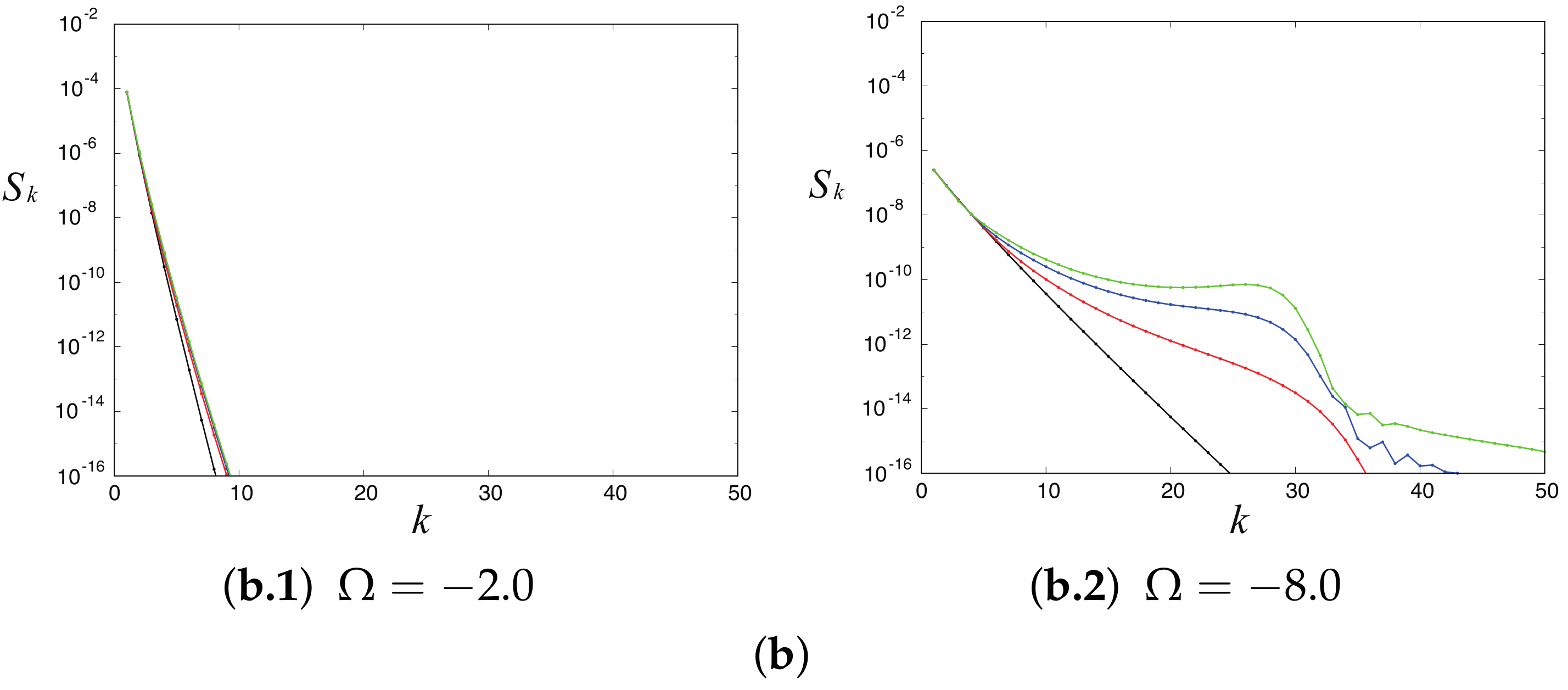
4.2. Generation of Parasitic Capillary Waves

Figure 3, Figure 4 and Figure 5 show the time evolution of the wave profile $\tilde{y}(x,t)$, the slope $\theta (x,t)$, the surface energy ratio $E_{\mathrm{S}}\left(t\right)/E_{\mathrm{T}}\left(t\right)$, and the energy spectrum $S_k\left(t\right)$, respectively, of gravity-capillary waves on a linear shear current. The initial values at $t=0$ are set to the pure gravity waves in Figure 2 of which the values of the parameter $\gamma$, the shear strength $\Omega$, the wave speed c and the wave steepness $\alpha$ are summarized in Table 1. The surface energy $E_{\mathrm{S}}\left(t\right)$ and the total energy $E_{\mathrm{T}}\left(t\right)$ are given by (18) and (23), respectively, and the slope $\theta (x,t)$ and the energy spectrum $S_k\left(t\right)$ are defined, respectively, by

$${\displaystyle tan\theta (x,t)=\frac{y_{\xi }}{x_{\xi }}\mathrm{and}{S}_k\left(t\right)={a_k\left(t\right)}^2+{b_k\left(t\right)}^2(k=0,1,2,\cdots ,N/2),}$$

(27)

where $a_k\left(t\right)$ and $b_k\left(t\right)$ are the Fourier coefficients in (19). In all computations, the Weber number is fixed to $1/W_e=0.006$, and the number N of Fourier modes in (19) and (20) and the time increment $\Delta t$ of the 4th-order Runge-Kutta method for numerical integration of (12) and (13) are set to $N=256$ and $\Delta t=2\pi /2048$, respectively. Note that the time t is non-dimensionalized as shown in (6) and the period of pure gravity steady waves used as the initial values is equal to $2\pi$. In the previous paper [7], we examined the convergence and the stability of this computational method for parasitic capillary waves without a shear current in detail. Similarly, we determined the values of N and $\Delta t$ in this work such that an error tolerance $|E_{\mathrm{error}}\left(t\right)|<{10}^{-8}$ is satisfied for all t where the error index $E_{\mathrm{error}}\left(t\right)$ is defined by (23).

Figure 3a,b show the time evolution of the wave profile $\tilde{y}(x,t)$ and the slope $\theta (x,t)$ for the case of $\gamma =0.2$ and $0.1$, respectively. It is found that, in the presence of a linear shear current with $\Omega <0$, parasitic capillary waves can be generated on small-amplitude gravity waves, as shown in the two cases (a) $\gamma =0.2$ and $\Omega =-4.0$ with $\alpha =\mathrm{O}\left({10}^{-3}\right)$ and(b) $\gamma =0.1$ and $\Omega =-8.0$ with $\alpha =\mathrm{O}\left({10}^{-4}\right)$ where the values of the wave steepness $\alpha$ are summarized in Table 1.

Figure 4 and Figure 5 show the time evolution of the surface energy ratio $E_{\mathrm{S}}\left(t\right)/E_{\mathrm{T}}\left(t\right)$ and the energy spectrum $S_k\left(t\right)$ of the computed results in Figure 3, respectively. We can see that, when parasitic capillary waves are generated, namely in the two cases (a) $\gamma =0.2$ and $\Omega =-4.0$ and (b) $\gamma =0.1$ and $\Omega =-8.0$, the wave energy is transferred from gravity waves to capillary waves. These results indicate that, even for very small-amplitude waves such as the wave steepness $\alpha =\mathrm{O}\left({10}^{-3}\right)$ or $\mathrm{O}\left({10}^{-3}\right)$, a nonlinearity works for generation of parasitic capillary waves.

5. Discussions

The number of parasitic capillary waves generated on the face of gravity waves has been of interest and was estimated by Fedorov & Melville [11] by imposing the condition that the linear wave speeds of gravity and capillary waves are equal under the steady flow assumption. From [8] (Equation (2.23)), the expression for the linear wave speed in dimensional form is given by

$$c=\frac{\Omega }{2k}\pm \sqrt{\frac{g}{k}\left(1+\frac{T}{\rho g}{k}^2\right)+{\left(\frac{\Omega }{2k}\right)}^2}.$$

(28)

While the background shear changes the (long) gravity wave speed, but affects little the (short) capillary wave speed, which can be approximated, from (28), by

$$c^2=\frac{T}{\rho }{k}_{\mathrm{cap}},$$

(29)

where $k_{\mathrm{cap}}$ is the capillary wavenumber and is assumed large. Then, from (7) along with (29), $k_{\mathrm{cap}}$ can be estimated, in terms of the Weber number $We$, by

$$\frac{k_{\mathrm{cap}}}{k}=\frac{We}{2\pi }\simeq 26.5,$$

(30)

where $1/We=0.006$ has been used in our computations. This is approximately the wavenumber, at which the short wave energy grows, as shown in Figure 5. The ratio between the gravity and capillary wavelengths is ${\lambda }_{\mathrm{cap}}/\lambda =1/26.5$ so that the number of capillary waves over the front half of the underlying gravity wave is about 13, independent of the shear strength $\Omega$. As can be seen in Figure 3, the argument of Fedorov & Melville [11] seems to provide an estimate that is consistent with our numerical solutions. Nevertheless, as our solutions are time-dependent and the excited parasitic capillary waves are modulated, the validity of this argument needs to carefully examined.

As pointed out in the preceding section, the generation of parasitic capillary waves, or the transfer of energy from gravity waves to capillary waves, is a nonlinear process that occurs even for small-amplitude waves in the presence of a linear shear. Therefore, it is of interest to find out which terms in the evolution equations are responsible for the generation of parasitic capillary waves. Considering that parasitic capillary waves can be generated on small-amplitude gravity waves, once these terms are identified, the evolution equations might be able to be simplified.

For such small-amplitude waves, we may approximate the free surface conditions (12) and (13) by neglecting high-order nonlinear terms by assuming that $x_{\xi }-1$, $x_{\xi \xi }$, y, $y_{\xi }$, $y_{\xi \xi }$, ${\varphi }_{\xi }-1$, $\psi$, ${\psi }_{\xi }$ are all small. This approximation allows us to examine which nonlinear terms are directly related to the generation of parasitic capillary waves. As a result, it is found that only one nonlinear term in the kinematic condition (12) is mainly responsible for the generation of capillary waves, and that the free surface conditions (12) and (13) can be approximated as

$$\begin{array}{ccc}{y}_t& =& -\left({\displaystyle {\psi }_{\xi }+\frac{\Omega }{c}y{y}_{\xi }}\right)\hfill \end{array},$$

(31)

and

$$\begin{array}{c}{\displaystyle {\varphi }_t-\mathcal{H}\left[{\displaystyle {\psi }_{\xi }+\frac{\Omega }{c}y{y}_{\xi }}\right]+\frac{1}{2}\left[1+2\{(1-x_{\xi })-(1-{\varphi }_{\xi })\}\right]+\frac{1}{c^2}y}\hfill \\ {\displaystyle +\frac{\Omega }{c}\left[y-\psi +y\{(1-x_{\xi })-(1-{\varphi }_{\xi })\}\right]-\frac{2\pi }{W_e}{y}_{\xi \xi }=B\left(t\right).}\hfill \end{array}$$

(32)

Compared with (12)–(13), notice that we include the second-order nonlinear terms with $\Omega$ are kept while all other terms are linearized.

Figure 6 compares the computed results for the wave profile $\tilde{y}(x,t)$ and the slope $\theta (x,t)$ at $t=3\pi$ using the approximate free surface conditions (31) and (32) with those using the original fully nonlinear conditions (12) and (13) for two cases: (a) $\gamma =0.2$ and $\Omega =-4.0$ and (b) $\gamma =0.1$ and $\Omega =-8.0$. It is found that the weakly nonlinear solutions using (31) and (32) reasonably well approximate the fully nonlinear solutions using (12) and (13) for small-amplitude waves. Therefore, the approximate evolution equations given by (31) and (32) would be useful to study the generation of parasitic capillary waves on small-amplitude gravity waves with a linear shear current.

6. Conclusions

We have numerically investigated the generation of parasitic capillary waves on gravity waves with a linear shear current. For fully nonlinear computation of this phenomenon, we have adopted the Unsteady Hodograph Transformation (UHT) method that conformally maps the flow domain onto the lower half of a complex plane, or the $\zeta$-plane, as shown in Section 2. The time-varying water surface is always mapped onto the real axis $\eta =0$, and the free surface conditions are transformed into (12) and (13) in the $\zeta$-plane. This method of computation enables us to obtain highly accurate solutions for a wide range of the wave steepness, the shear strength, and the surface tension.

We have computed the time evolution of the wave profile $\tilde{y}(x,t)$, the slope $\theta (x,t)$ of the water surface, the surface energy ratio $E_{\mathrm{S}}/E_{\mathrm{T}}$, and the energy spectrum $S_k\left(t\right)$ defined by (27) using the UHT method, as shown in Figure 3, Figure 4 and Figure 5. The initial values at $t=0$ are set to pure gravity steady waves whose curvature $\kappa$ near the crest can be relatively large even for small-amplitude waves in the presence of a linear shear current, as shown in Figure 2. Numerical solutions have shown that the linear shear current with the shear strength $\Omega <0$ makes the energy transfer from gravity waves to capillary waves more effectively so that parasitic capillary waves can be generated even if the amplitude of underlying gravity waves is very small. For example, the wave steepness $\alpha =\mathrm{O}\left({10}^{-3}\right)$ or $\mathrm{O}\left({10}^{-3}\right)$ is large enough for the generation of parasitic capillary waves, which is unlikely to happen for the case of $\Omega =0$.

Therefore, under the assumption of small wave amplitude, we have found the approximate free surface conditions (31) and (32), which might be useful for a theoretical study. The computed results using this approximate model showed that the weakly nonlinear terms with $\Omega$ play a key role in the generation of parasitic capillary waves on small-amplitude gravity waves with a linear shear current, as demonstrated in Figure 6.

In future investigations, it would be worthwhile to take viscous effects into consideration and compare the computed results with experimental data when they are available.

References

1. Peregrine, D.H. Interaction of water waves and currents. Adv. Appl. Mech. 1976, 16, 9–117. [Google Scholar]
2. Perlin, M.; Schultz, W. Capillary effects on surface waves. Annu. Rev. Fluid Mech. 2000, 32, 241–274. [Google Scholar] [CrossRef]
3. Cox, C. Measurements of slopes of high-frequency wind waves. J. Mar. Res. 1958, 16, 199–225. [Google Scholar]
4. Longuet-Higgins, M. The generation of capillary waves by steep gravity waves. J. Fluid Mech. 1963, 16, 138–159. [Google Scholar] [CrossRef]
5. Dommermuth, D. Efficient simulation of short and long-wave interactions with applications to capillary waves. J. Fluids Eng. 1994, 116, 77–82. [Google Scholar] [CrossRef]
6. Jiang, L.; Lin, H.-J.; Schultz, W.; Perlin, M. Unsteady ripple generation on steep gravity-capillary waves. J. Fluid Mech. 1999, 386, 281–304. [Google Scholar] [CrossRef] [Green Version]
7. Murashige, S.; Choi, W. A numerical study on parasitic capillary waves using unsteady conformal mapping. J. Comput. Phys. 2017, 328, 234–257. [Google Scholar] [CrossRef] [Green Version]
8. Choi, W. Nonlinear surface waves interacting with a linear shear current. Maths Comput. Simul. 2009, 80, 29–36. [Google Scholar] [CrossRef]
9. Murashige, S.; Choi, W. Stability analysis of deep-water waves on a linear shear current using unsteady conformal mapping. J. Fluid Mech. 2020, 885, A41. [Google Scholar] [CrossRef]
10. Guo, D.; Tao, B.; Zeng, X. On the dynamics of two-dimensional capillary-gravity solitary waves with a linear shear current. Adv. Math. Phys. 2014, 2014, 480670. [Google Scholar] [CrossRef]
11. Fedorov, A.V.; Melville, W.K. Nonlinear gravity-capillary waves with forcing and dissipation. J. Fluid Mech. 1998, 354, 1–42. [Google Scholar] [CrossRef] [Green Version]
Figure 1. Two-dimensional periodic motion of deep-water gravity-capillary waves on a linear shear current and conformal mapping of the flow domain into a complex plane. (a) The z-plane ( z = x + i y ); (b) The ζ -plane ( ζ = ξ + i η ).
Jmse 09 01217 g001
Figure 2. Pure gravity steady waves progressing in permanent form on a linear shear current with the shear strength Ω . The slope θ ( 0 ) ( x ) and the curvature κ ( 0 ) ( x ) are given by (26), and the parameter γ is defined by (24). The number of Fourier modes in (25) is set to M = 128 . (a) γ = 0.2 (black line : Ω = 0.0 , red line : Ω = 1.0 , blue line : Ω = 2.0 , green line : Ω = 3.0 , magenta line : Ω = 4.0 ). (b) γ = 0.1 (black line : Ω = 0.0 , red line : Ω = 2.0 , blue line : Ω = 4.0 , green line : Ω = 6.0 , magenta line : Ω = 8.0 ).
Jmse 09 01217 g002
Figure 3. Time evolution of the wave profile y ˜ ( x , t ) and the slope θ ( x , t ) of gravity-capillary waves on a linear shear current with the shear strength Ω . The initial values are set to pure gravity waves in Figure 2. See Table 1 for the parameter values of the initial waves. The parameter γ is defined by (24). 1 / W e = 0.006 , N = 256 and Δ t = 2 π / 2048 . (a) γ = 0.2 (red line : Ω = 1.0 , blue line : Ω = 2.0 , green line : Ω = 3.0 , magenta line : Ω = 4.0 ). (b) γ = 0.1 (red line : Ω = 2.0 , blue line : Ω = 4.0 , green line : Ω = 6.0 , magenta line : Ω = 8.0 ).
Jmse 09 01217 g003aJmse 09 01217 g003bJmse 09 01217 g003c
Figure 4. Time evolution of the surface energy ratio E S ( t ) / E T ( t ) of the computed results in Figure 1, Figure 2, Figure 3. The surface energy E S ( t ) and the total energy E T ( t ) are given by (18) and (23), respectively. The parameter γ is defined by (24). (a) γ = 0.2 (red line : Ω = 1.0 , blue line : Ω = 2.0 , green line : Ω = 3.0 , magenta line : Ω = 4.0 ). (b) γ = 0.1 (red line : Ω = 2.0 , blue line : Ω = 4.0 , green line : Ω = 6.0 , magenta line : Ω = 8.0 ).
Jmse 09 01217 g004
Figure 5. Time evolution of the energy spectrum S k ( t ) of the computed results in Figure 3. S k ( t ) is given by (27) and the parameter γ for is defined by (24). (black line : t = 0 , red line : t = π , blue line : t = 2 π , green line : t = 3 π ). (a) γ = 0.2 ; (b) γ = 0.1 .
Jmse 09 01217 g005aJmse 09 01217 g005b
Figure 6. Comparison of the computed results of the wave profile y ˜ ( x , t ) and the slope θ ( x , t ) at t = 3 π using the approximate free surface conditions (31) and (32) with those using the fully nonlinear conditions (12) and (13). The initial values are set to pure gravity waves in Figure 2. See Table 1 for the parameter values of the initial waves. The parameter γ is defined by (24). 1 / W e = 0.006 , N = 256 and Δ t = 2 π / 2048 . (black line : the fully nonlinear solutions using (12) and (13), red line : the weakly nonlinear solutions using (31) and (32)). (a) γ = 0.2 and Ω = 4.0 ; (b) γ = 0.1 and Ω = 8.0 .
Jmse 09 01217 g006