Experimental Study on the Shear Band of Methane Hydrate-Bearing Sediment

Abstract

The occurrence of a shear band is often thought as the precursor of failure. To study the initiation of shear banding in gas hydrate-bearing sediments, two groups of triaxial compression tests combined with a CT (computer tomography) scan were conducted by triaxial CT-integrated equipment under two confining pressures and seven hydrate saturations. The macro stress–strain curves and the corresponding CT scanning images of the micro-structure and the distribution of the components were obtained. The geometric parameters of the shear bands were measured based on the CT images at four typical axial strains, respectively. The distribution characteristics of soil particles, water, hydrate and gas were also analyzed. It is shown that the existence of methane hydrate changes the mechanical property of hydrate-bearing sediment from plastic failure to brittle failure when the hydrate saturation is over 13%, which occurs in the range of the tests in this paper. The peak of the deviatoric stress increases with the hydrate saturation. The shear band is in either a single oblique line or inter-cross lines depending on the hydrate saturation, the effective confining pressure and the initial distribution of the gas hydrate. Most of the shear band surfaces are not straight, and the widths of the shear bands are almost non-uniformly distributed.

1. Introduction

The initiation of a shear band, a local zonal region with concentrated deformation [1], is related mainly to instability and bifurcation. The instability is formulated by considering small perturbation in field variables. Triaxial or plain strain experiments are often used to study the deformation instability and the failure modes in geomechanics. The results show clearly that the uniform response is followed by the occurrence of a diffused and heterogeneous deformation, after which a shear band forms. The development of a shear band is often the main reason of landslide and foundation pit failure [2].

The shear band is formed under the combined action of the external load and intrinsic natures of the soil layer and rock [3]. Concerns regarding the shear band are when to initiate and how to evolve.

Generally, shear banding initiates from the softening of some local areas and then evolves into one or an inter-cross zonal area with concentrated deformation. In the macro point of view, a shear band is determined by the density, status of stress and strain, constitutive relation, etc., of the soil layer. From the micro point of view, the formation of a shear band results from the local heterogeneous deformation during the rearrangement of the particles of the soil layer [4,5].

Rice and Rudnick [6,7] obtained the initial condition of shear banding in saturated soils by using the perturbation method. The status of stress and strain, plastic flow rule and dissipation rate of pore pressure were found to be the controlling factors. Vardoulakis [8,9] found that the initiation and evolution of the shear band were determined by the properties of the soil layer and the load characteristics by bifurcation analysis. Bazant et al. [10] presented a critical condition of shear banding based on the non-local theory. Zbib and Aifantis [11], Lu et al. [12] and Wang et al. [13] investigated the initiation and evolution of shear banding based on the plastic theory of strain gradient.

The factors affecting the width and direction of shear banding are mainly the internal angle, dilation angle, grading curve of grains, form of grains and confined pressure. It is difficult to consider all of these factors in the analysis. Therefore, experiments are often used to investigate the characteristics and main controlling factors during the initiation and evolution of shear banding. Stereoscopic camera [14] charge-coupled devices (CCD) were used in the experiments to study the macro and micro characteristics of shear banding evolution, such as the rotation of grains and slide and the width and direction [15,16,17]. Oda et al. [18] and Nemat-Nasser et al. [19] adopted X-ray and optical methods to study the micro structure of shear banding. They observed large pores inside the shear band and the acute variation of the grains’ rotation. The width of the shear band was about 7–8 times the average.

A few studies on shear band in gas hydrate bearing sediment (GHBS) have been carried out. Kato et al. [20] analyzed the TC (triaxial compression) and PSC (plane strain compression) tests results and concluded that the thickness of shear band in MH (methane hydrate)-bearing sand appeared to be thinner than that in pure sand, and more particles crushing occurred inside the shear band in MH-bearing sand. Jiang et al. [21] simulated the occurrence of shear band by distinct element method (DEM). The results show that the occurrence of shear band in GHBS is due to the damage of cohesion among numerous grains. Sun [22] observed the occurrence and evolution of shear band in GHBS by triaxial apparatus combining with CT. The effects of the saturation of gas hydrate and the confined pressure were studied. Yoneda et al. [23] studied the inner structure and the failure mechanism of krypton hydrate bearing sand by using micro-focus X-ray CT in a novel micro triaxial testing apparatus via PIV (particle image velociraptor) method. They found that the structure of the sediment in the shear band significantly changed due to the movement and rotation of the soil particles and the hydrate, the inclination angle of the shear band increased with hydrate saturation. Pinkert et al. [24] postulated two micro-scale mechanisms of failure to explain the sudden strength loss, occurrence of double shear banding and differences in post-peak behaviour of cemented hydrate bearing sand, and found that the occurrence of double shear bands is in general agreement with the results of DEM by Jiang et al [25]. However, the knowledge on the initiation and evolution of shear band in GHBS is very limited. The formation of gas hydrate in sand not only causes the components of sediment from three phases (solid/liquid/gas) to four phases (solid/liquid/gas/hydrate), but also enhances the cementation among grains and decreases the porosity, which leads to the mechanism of initiation and evolution of shear band more complicated in GHBS than in common soils.

In regard to the points above, the initiation and evolution of shear banding in GHBS will be studied by triaxial experiments combined with CT. Besides the macro stress–strain curves, micro images at different strains are obtained to analyze the distribution of gas hydrate and the changes of pores during the evolution of shear banding, which helps us to understand the shear banding in GHBS further.

2. Equipment and Test Method

2.1. Simple Introduction of Equipment

The integrated equipment combined a CT (computer tomography) and a lightweight triaxial apparatus, developed by Qingdao Institute of Marine Geology, China Geological Survey, which was used to carry out the experiments (shown in Figure 1; Figure 2). The integrated equipment consisted of a core holder (reactor), which can be penetrated by X-ray, a controlling unit for axial load and displacement, a controlling unit for pressure and temperature and a set of data collection unit.

The maximum allowable axial load of the triaxial apparatus is 50 kN. The displacement rate can be controlled in the range of 0.01 mm/min to 3.80 mm/min. The maximum/minimum allowable displacement of the axial load head is ±12.5 mm. The allowable confined pressure of the sample in triaxial pressure cell is in the range of 0 to 30 MPa. The gas for gas hydrate synthesis is inputted from a hole set at the center of the bottom. A vent valve is set at the top of the reactor for the gas emission and collection.

The CT, model of Phoenix∣V Tome∣X, is produced by GE Company and consisted of two sets of X-ray source (μm and nm), a three-dimensional turntable and a flat panel detector (shown in Figure 1) [26]. The detectable area is 20 cm × 20 cm. The core holder is placed at the turntable, which can rotate 360° during CT scan. It brings the holder the characteristics of light weight, strong penetrability and high strength, made by titanium alloy strengthened by carbon fiber. The size of the sample is diameter × height = 25 mm × 50 mm.

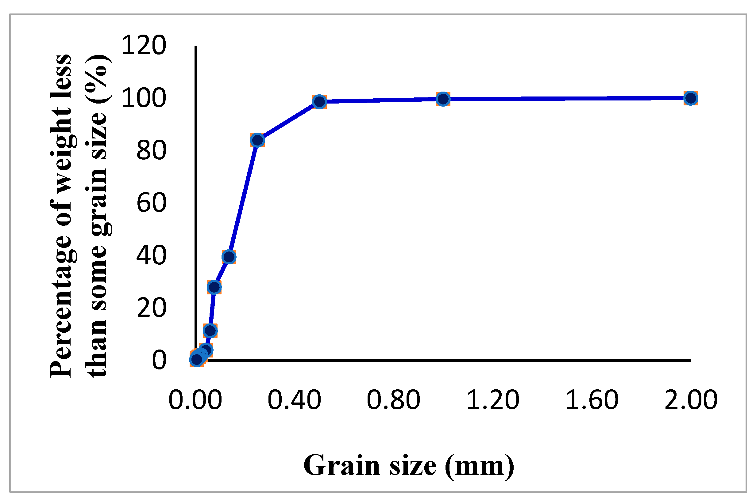
2.2. Material and Preparation of Specimen

In this study, the methane hydrate-bearing sandy samples were synthesized for experiments. The grain size distribution of the sand, measured by means of sieve analysis, is shown in Figure 3. The main physical parameters of the sand are as follows: the specific gravity 2.65, relative density 54%, dry bulk density 1600 kg/m³, porosity 0.4. These parameters are measured according to the standard for test methods of earth works GB/T50123-2019. During preparing specimens, the wet and dry sand were weighted according to the designed hydrate saturation and mixed fully with each other. Then, the wetting sand was put into the membrane and compacted in four layers.

The procedures for sample preparation as follows:

(1)

During sample preparation, deionized water was used, and the required water was measured by a small graduated cylinder. The required water content was computed by Equation (1). The water was mixed up fully with dry sand with a mass of m_s. The mixture of sand and water was divided into four equal parts.

(2)

A rubber membrane wrapped around the lower part of the core of sample holder. Then, a set of metal holding mold coated the rubber membrane. The four parts of the mixture were put in the membrane in sequence. Each part was compacted by a weight to form a sand layer with a height of 12.5 mm. The interface between every two layers was roughened by a brush.

$$S_h=\frac{w\cdot {\rho }_s\cdot \rho }{0.87\cdot {\rho }_w\cdot \left[(1+w)\cdot {\rho }_s-\rho \right]}$$

(1)

in which S_h is the hydrate saturation of GHBS sample, w is the water content, ρ_w is the density of water, ρ_s, ρ are the dry density and density of the sand sample, respectively.

Synthesis of methane hydrate-bearing samples:

The GHBS sample was prepared by gas saturation method. The gas pressure, gas mass, temperature and water mass were estimated by the phase equilibrium curve of the gas, water and hydrate three phases [27]. The water mass was measured strictly according to the value estimated by the phase equilibrium curve. Sufficient gas was supplied during synthesis of gas hydrate. By this way, the mass of gas hydrate was controlled at the designed value. The detailed procedures of the synthesis of gas hydrate-bearing samples are as follows:

Firstly, the prepared sand sample was placed in the pressure cell of the triaxial apparatus. The measured water was injected slowly into the sand sample by a graduated cylinder.

Secondly, the opening of the air pump, cycle refrigerating machine, control board and the control software was operated in sequence. The temperature was controlled to be 14 °C by the cycle refrigerating machine.

Thirdly, the bumps for providing the confining pressure and axial load were adjusted. The gas in the systems of confining pressure and axial pressure was exhausted. Then, the bumps for providing the confining pressure and axial load were set up as the mode of synchronous pressing. The discharge of the bump of confining pressure was set as 32 mL/min. The confining pressure and the gas pressure were increased gradually till the designed value was reached. During the synthesis of gas hydrate, the gas pressure was kept around 8.9 MPa. The temperature was kept as 0.1 °C.

Finally, the synthesis process was retained for 72 h under the conditions of the designed pressure and temperature. The gas consumed by synthesis of hydrate was estimated by the drop of gas pressure and the gas state equation (Equations (2) and (3)). Once the consumption of gas mass was determined, the mass and the saturation of gas hydrate could be computed according to the structure formula CH₄·6H₂O [28]. The estimated saturation can be used to certify the value determined by Equation (1).

(a) If the pressure is not too high and temperature is near the normal atmospheric temperature, the ideal gas state equation can be used:

$$\begin{array}{c}{ \mathrm{P}}_1^0{\mathrm{V}}_1/{\mathrm{T}}_1={\mathrm{P}}_2^0{\mathrm{V}}_2/{\mathrm{T}}_2\\ {\mathrm{P}}_1{\mathrm{V}}_1/{\mathrm{T}}_1={\mathrm{P}}_2{\mathrm{V}}_2/{\mathrm{T}}_2\\ {\mathrm{V}}_{\mathrm{gass}}={\mathrm{V}}_2-{\mathrm{V}}_1=\frac{\left({\mathrm{P}}_1^0-{\mathrm{P}}_1\right){\mathrm{V}}_1{\mathrm{T}}_2}{{\mathrm{T}}_1{\mathrm{P}}_2}\\ {\mathrm{V}}_{\mathrm{hs}}={\mathrm{V}}_{\mathrm{gass}}/164\end{array}$$

(2)

in which P₁, ${\mathrm{P}}_1^0$, P₂ are the standard atmosphere pressure, the initial and steady state gas pressure in the pressure cell; T₁, T₂ are the environmental temperature (22 °C) and the temperature at standard state (273.15 K); V₁, V₂ are the volume of the cell (10 mL), the gas volume at the standard state corresponding to the initial pressure and the pressure at steady state, respectively; V_gass, V_hs are the required gas volume at the standard state and the volume of synthesis gas hydrate, respectively.

(b) If the pressure and the temperature are deviated from ordinary pressure and normal atmospheric temperature too much, the van der Waals equation should be used:

$$\left(\mathrm{P}+\frac{{\mathrm{an}}^2}{{\mathrm{V}}^2}\right)\left(\mathrm{v}-\mathrm{nb}\right)=\mathrm{nRT}$$

(3)

in which a is a constant related with the intermolecular attraction, b is the volume of a single molecule, n = m/M named number of moles, m is the gas mass, M is the Molar mass, R is the Boltzmann constant. As the temperature 0.1 °C during synthesis of gas hydrate in our sample preparing is far lower than the normal atmospheric temperature, the van der Waals equation is used to estimate the consumption of gas mass.

2.3. Test Method and Process

Triaxial compression test combined with CT scan:

After preparation of the sample, the shear rate, ultimate displacement and the ultimate axial load were set as 0.1 mm/min, 10 mm and 5 × 104 N, respectively. Then, the triaxial compression tests were carried out. The stress, axial strain data were recorded. Due to the small size of the sample, the ring strain gauge is difficult to install to measure the lateral strain. Meanwhile, the sample contained some gas, so the volume could not be measured by the drained water. Therefore, the volume strain was not recorded.

The combined triaxial tests and CT scan were divided into two groups: the effective confining pressure 1 MPa and the hydrate saturations 0%, 25%, 38%, 50%, respectively; the effective confining pressure 3 MPa and the hydrate saturations 0%, 13%, 40%, respectively. When the axial strain arrived at 0%, 5%, 10% and 15%, the axial load was stopped and CT scan was conducted in about 20 min.

3. Results and Discussion

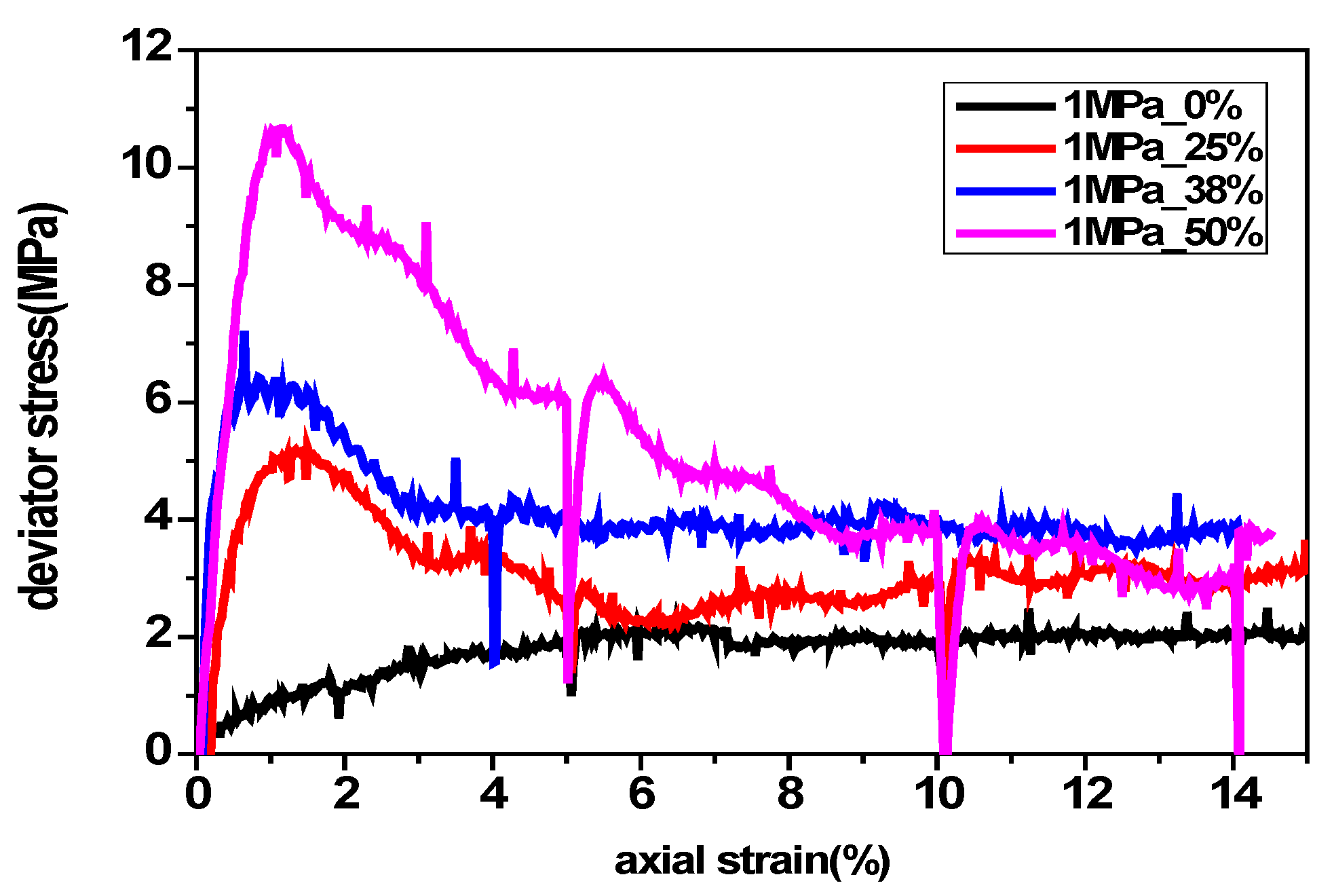
3.1. Results at the Effective Confining Pressure 1 MPa

Figure 4 shows the stress–strain curves under the effective confining pressure of 1 MPa. It is shown that the deviatoric stress increases slowly with the axial strain till the peak; the peak is 7% for the sample without gas hydrate (S_h = 0%). The sample behaves as a typical plastic failure mode in this case. However, the deviatoric stress increases rapidly with the strain and reaches the peak at strains between 1% and 1.5% and then rapidly drops for the hydrate saturation of S_h = 25%, 38% and 50%, respectively. The strain changes very slowly with the pressure after it is over 6%. These samples behave as obvious brittle failure modes.

Overall, for hydrate-bearing samples, the larger the hydrate saturation is, the larger the shear strength is, and the strain softening (the decrease degree of the deviatoric stress from the peak) is more obvious. The residue shear strength tends to be a constant and higher than that of the sample without gas hydrate. The stress–strain curves indicate that the methane hydrate decreases the porosity and cements the grains, so both the density and the strength of the sample increase. These factors turn the hydrate-bearing samples brittle from plasticity. It should be noted that the sudden drop of stress in the curves is caused by the decrease of the axial load during the CT scan, although we tried to keep the load unchanged. The required axial load becomes larger with the increase of hydrate saturation, but the load is more difficult to keep.

In this section, the initiation and evolution of shear banding in the hydrate-bearing samples will be discussed mainly based on the CT images (as shown in Figure 5 Figure 6 Figure 7 Figure 8).

At S_h = 50%, the initial distribution of the gas hydrate looks uniform, but the pore space in the middle of the sample increases in a sheet type from the top-right to the bottom-left with the increase of the axial strain (as shown in Figure 5). At the strain of 10%, a wide shear band (length = 36.1 mm, width = 9.3 mm, angle = 45°) occurs that is left-inclined and across both sides of the sample. However, there are not any fractures and large displacement dislocations in the sample. The shape of the sample is like a drum (wider in the middle and thinner at both ends) at a large strain. At the strain of 15%, another right-inclined shear band (length= 36.1 mm, width = 9.3 mm, angle = 45°) occurs, and finally two inter-cross shear bands form in the middle of the sample.

Figure 6 is the distribution image of the hydrate, soil particle, water and gas at S_h = 50%. The initial pore is not uniformly distributed and there is an incline band full of gas. At the strain of 15%, an area filled with gas in the right side of the sample can be observed. This space is caused by the non-uniform compaction during the preparation of the specimen and hydrate synthesis. The shear band can be seen only from some sections of scanning images at a certain strain, i.e., the shear band forms only in some shallow area of the sample and does not break through the whole section.

At S_h = 38%, a curvilinear shear band (length = 39.1 mm, width = 3.3 mm, angle = 30°~60°) is formed at the axial strain of 5% (Figure 5). The width of the shear band increases while the length and the angle of the shear band gradually decreases because of the compression of the sample with the increase of the axial strain. When the strain arrives at 10%, both the length and the width of the shear band develop further. At the strain of 15%, an obvious deformation dislocation area occurs in both sides of the sample. There is a crush at the upper and lower parts of the shear band.

From the distribution images of the hydrate, soil particles, water and gas at S_h = 38% (Figure 7), we can see that there is a narrow strip and an area at the lower right of the sample with high contents of gas and water, i.e., shear banding. The shear band can be easily observed in the left incline when the strain is 10% from the images in the scanning directions of 1 and 2. However, from other images at the strain of 15% in the scanning directions of 1 and 2, there are not any shear bands to be found. From the front and right view of the 3D images, the geometry of shear banding is different in different scanning directions. Therefore, the real structure of the shear band should be determined by a large amount of CT scanning images.

From Figure 8, a left-inclined shear band (length = 31.6 mm, width = 4.3 mm, angle = 30°) forms at the axial strain of 5% at S_h = 25%. The width of the shear band increases obviously when the strain increases to 15% from the scanning images in the front scanning direction. An obvious loose collapse occurs in the lower end of the sample. In the right direction, a right-inclined shear band can be seen (length = 39.9 mm, width = 2.0 mm, angle = 52°), which breaks through almost all the height of the sample when the strain reaches 10%. When the strain increases to 15%, the angle of the shear band decreases a little due to the vertical compression of the sample. The sample appears to be a whole loose collapse.

From the distribution images of the hydrate, soil particle, water and gas at S_h = 25% (as shown in Figure 8), it can be seen that there is obviously a shear band in the sample. The scanning images in different directions show the different profiles of the shear band. It is found that there are several discontinuous shear bands in the sample when the axial strain is 10%. Because of more pores and gas concentrated in the middle of the sample and more soil particles distributed at the two ends, the strength at the middle part of the sample is less than that near the two ends. Thus, the shear band first initiates in the middle of the sample.

If the sample contains no gas hydrate (Sh = 0%), no shear banding in the sample occurs. The sample is shown to look like a drum at a strain of 15% (Figure 5).

From the CT scanning images, we can see that the pores are not distributed uniformly during preparing the specimen, so the gas hydrate is synthesized heterogeneously in the sample. Subsequently, the shear bands initiate in weak areas of the sample and in different geometric forms. Therefore, in order to understand the evolution of shear banding better, the sample preparation of hydrate-bearing sediment needs to be further improved.

3.2. Results at the Effective Confining Pressure 3 MPa

In this section, we will discuss the mechanical properties and the evolution of shear banding at the hydrate saturations of S_h = 0%, 13% and 40% and the effective confining pressure of 3 MPa. From the stress–strain curves (Figure 9) and the CT scanning images (Figure 10), it can be found that the deviatoric stress increases with the increase of strain and reaches the peak when the strain is 5% and then keeps steady afterwards at S_h = 0, i.e., the sample behaves in a typical plastic mode. The corresponding CT scanning images show that there is not any emergence of shear banding in the sample. At S_h = 13%, the deviatoric stress rapidly increases with the strain till the peak strain of 1.5%, and then the sample behaves in plastic failure mode. The corresponding CT scanning images show that the diameter of the top of the sample is larger than the other parts and no shear bands are observed. At S_h = 40%, the deviatoric stress also increases rapidly with the strain till the peak strain of about 2% is reached, and then the stress decreases rapidly till the strain of 5%. The sample behaves in the brittle failure mode. The corresponding CT scanning images show that a shear band extends only along part of the middle section (length = 29.7 mm, width = 3.6 mm, angle = 62°). When the strain is 10%, the shear band increases in length and runs through the left side of the sample. When the strain arrives at 15%, the shear band extends to the right of the sample (length = 32.0 mm), while there are little changes in the width and the angle. The shear band is left-inclined and across both sides of the sample. Moreover, there is an obvious crack at the lower left of the sample, but the shear band has not yet run through the right side of the sample. The top of the sample becomes denser and thicker.

From the distributions of the hydrate, gas and soil particles (Figure 11 and Figure 12), it can be seen that the hydrate-bearing samples are very non-uniform at the confining pressure of 3 MPa. Several gas strips distribute at the bottom and the side of the sample at S_h = 13%. A gas strip distributes only at the side of the sample at S_h = 40%. Obviously, the saturation of the gas at the bottom of the sample is the highest. The increase of the gas leads to the increase of the compressibility of the sample; thus, the plasticity of the sample increases, resulting in the difficult initiation of shear banding in these cases. These phenomena are in coincidence with the stress–strain curves shown in Figure 9. There are not any shear bands formed in the plastic sample at S_h = 13%, but there is a shear band formed extending only partly in the sample in a brittle sample at S_h = 40%.

A comparison of the evolution of shear bands under two different confining pressures shows that the shear band is more difficult to initiate at the confining pressure of 3 MPa than at 1 MPa. It indicates that the initiation of a shear band depends not only on the hydrate saturation and soil skeleton but also on the confining pressure. The higher the hydrate saturation is, the denser the soil skeleton is and the more brittle the sample is, the more easily the shear band initiates. When the confining pressure is applied to the sample before the hydrate formation, the soil skeleton is compacted and the slide and rotation of the soil particles are also limited. Therefore, the confining pressure plays an important role in restraining the initiation of the shear band.

In general, the deviatoric stress of the sand samples without hydrate reaches the peak at the axial strain of about 7%, while it is 1–1.5% for the hydrate-bearing samples. It indicates that the existence of methane hydrate in sand samples increases the brittleness. The CT scanning images show that the shear band has obviously formed when the strain reaches about 5%, and at last develops gradually in types of single straight line, single arc line and crossing line. According to the previous studies on shear banding in rock and soil samples, shear bands initiate just near the peak deviatoric stress. Unfortunately, in this work, the initiation of shear banding cannot be exactly known because of a lack of scanning images at the strain of 1–1.5%.

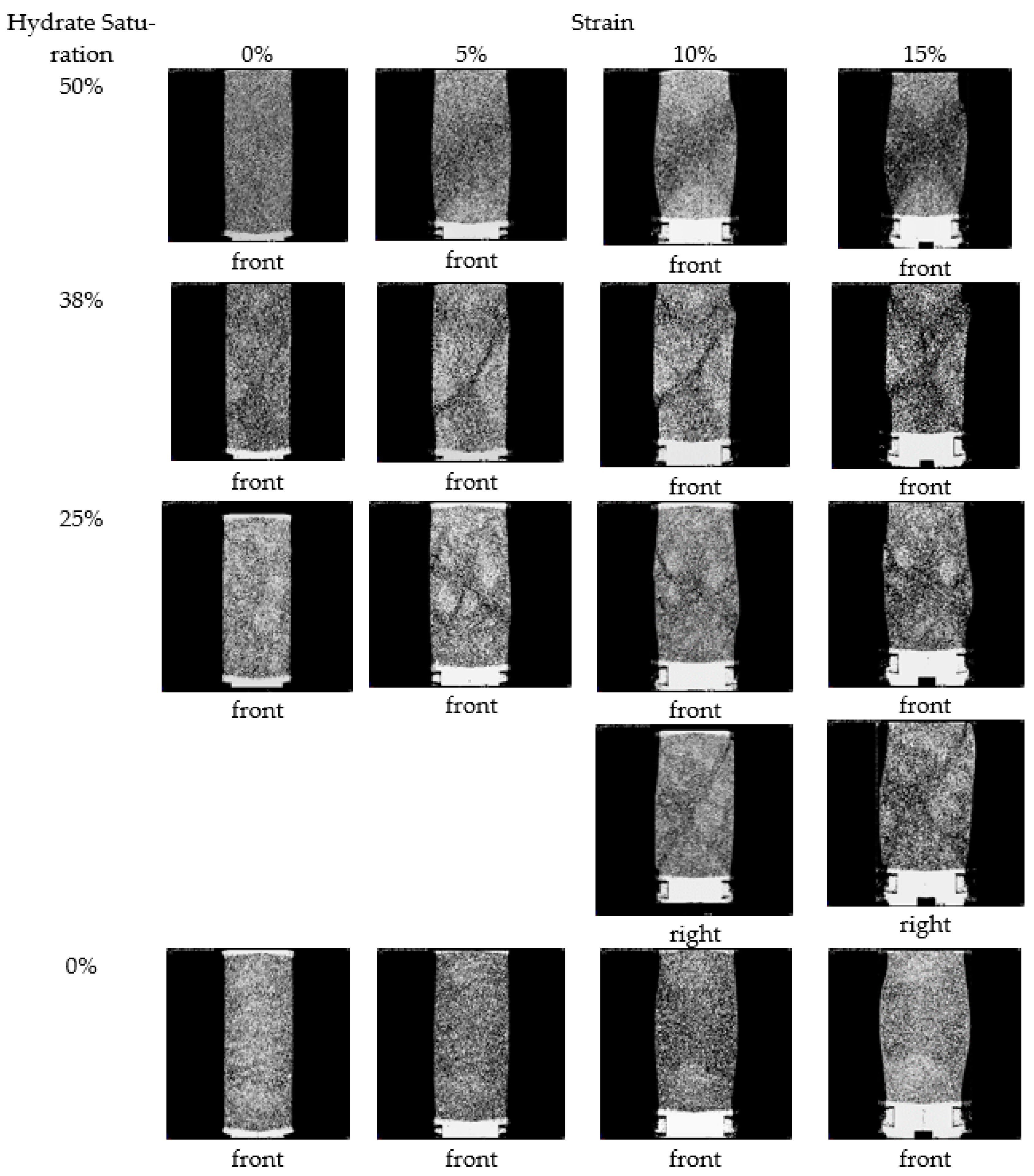
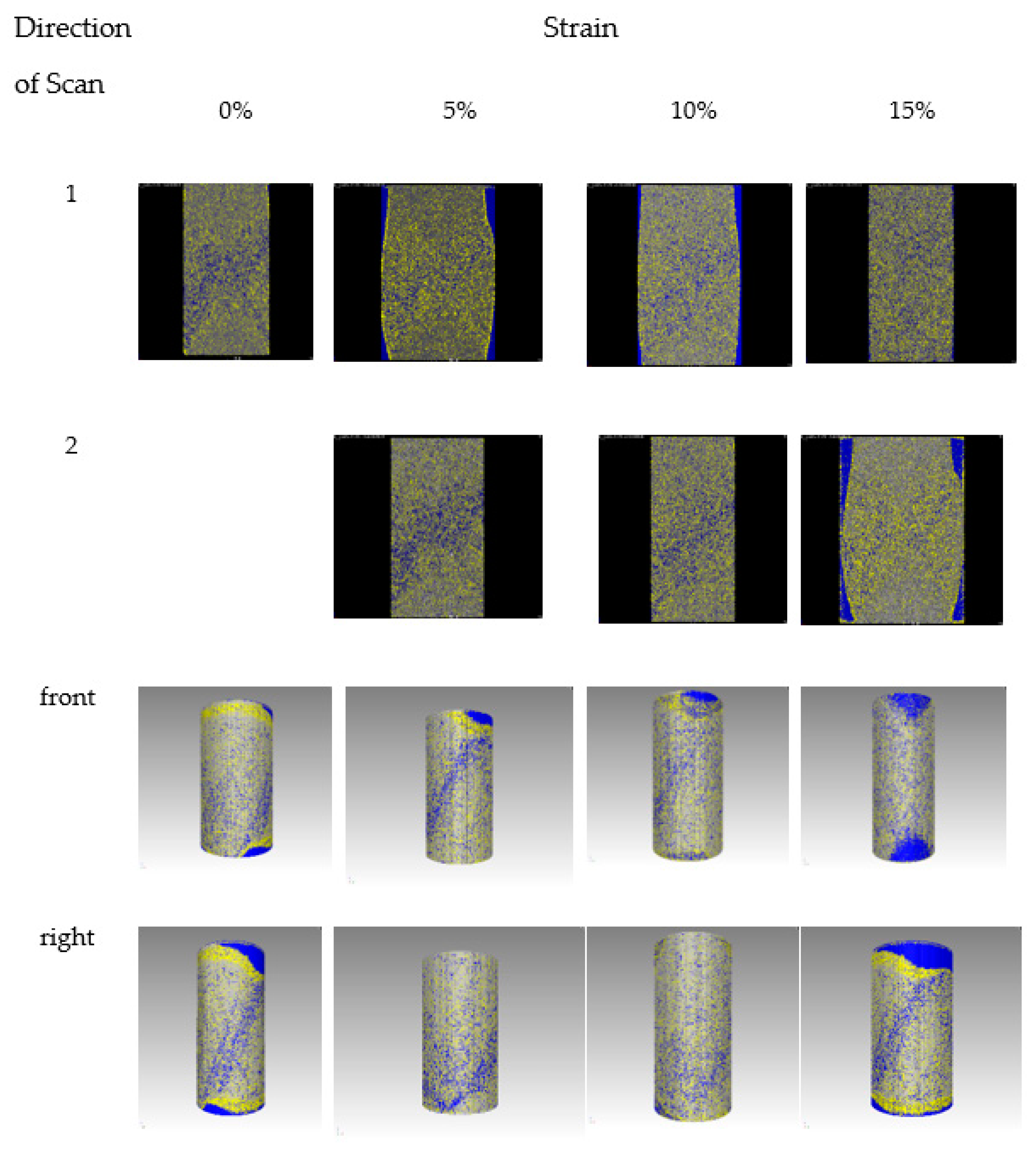
3.3. Geometrical Characteristics of Shear Banding

Table 1. The development of shear banding in geometrical parameters.

Confining Pressure	Hydrate Saturation	Parameters of Shear Band	Strain
			0%	5%	10%	15%
1 MPa	50%	L(mm)	0	0	36.1	36.1*2
		W(mm)	0	0	9.3	9.3*2
		φ (°)	0	0	46	46
1 MPa	38%	L (mm)	0	39.1	38	35.9
		W (mm)	0	3.3	3.5	4.0
		φ (°)	0	30–60	28–50	25–50
1 MPa	25%	L (mm)	0	39.1	38	35.9
		W (mm)	0	3.3	3.5	4.0
		φ (°)	0	30–60	28–50	25–50
3 MPa	40%	L (mm)	0	29.7	30.8	32.0
		W (mm)	0	3.6	4.5	4.7
		φ (°)	0	62	60	62

Note: * indicates two inter-cross shear bands.

is the summary of the scales of the shear band (length, width and angle) at different strain, hydrate saturation and confining pressure. Generally, the length of the shear band decreases a little with the increase of strain because of the vertical compression of the sample (except for S_h = 50%). The width of the shear band increases with strain, and the maximum is about 10 times the diameters of the soil particles. The angle of the shear band varies from 25° to 60° with the changes of the strain and hydrate saturation. However, when the confining pressure is 3 MPa, the angle of the shear band does not change with the strain, while the length and width of the shear band increase a little with the strain.

4. Conclusions

The macro triaxial compression test and micro-CT scanning test on methane hydrate-bearing sandy samples were carried out. The effects of the hydrate saturation and confining pressure were investigated. The main conclusions are as follows:

The existence of methane hydrate in sediments changes the mechanical properties. The samples behave as plastic characteristics when the saturation of the gas hydrate is less than 13%, Otherwise, the samples containing gas hydrate show brittle characteristics. The deviatoric stress of the hydrate-bearing samples reaches the peak when the axial strain is about 1%–1.5%, while the sand samples reach the peak at the axial strain of about 7%. In many cases, the shear band does not pass through the whole cross section.

With the changes of the hydrate saturation, confining pressure and the initial distribution of the hydrate, the shear band of the hydrate-bearing sample forms in several types: a straight line when the hydrate saturation is between 25% and 38%, and inter-cross lines when the hydrate saturation is around 50%. Most of the shear surfaces are non-straight, and the widths of the shear band are not uniform.

The initiation of the shear band becomes difficult when the confining pressure increases from 1 MPa to 3 MPa. The reason is that the skeleton of the sample is denser with the increase of the confining pressure. When the sliding and rotation of the soil particles are limited because of the applied load, the shear bands occur with more difficulty.

References

1. Roscoe, K.H. The influence of strains in soil mechanics. Geotechnique 1970, 20, 129–170. [Google Scholar] [CrossRef]
2. Lockner, D.A.; Byerlee, J.D.; Kuksenko, V.; Ponomarev, A.; Sidorin, A. Quasi-static fault growth and shear fracture energy in granite. Nature 1991, 350, 39–42. [Google Scholar] [CrossRef]
3. Lu, X.B.; Yang, Z.S.; Zhang, J.H. The evolution of shear bands of saturated soil. Int. J. Nonlinear Mech. 2000, 35, 21–26. [Google Scholar]
4. Muhlhaus, H.B.; Vardoulakis, I. The thickness of shear bands in materials granular. Geotechnique 1987, 37, 271–283. [Google Scholar] [CrossRef]
5. Zhang, Q.H.; Zhao, X.H. Study on mechanism of localized shear band formation in clay. Rock Soil Mech. 2002, 1, 31–35. [Google Scholar]
6. Rice, J.R. On the stability of dilatant hardening for saturated rock masses. J. Geophys. Res. 1975, 80, 1531–1536. [Google Scholar] [CrossRef] [Green Version]
7. Rudnicki, J.W.; Rice, J.R. Conditions for the localization of deformation in pressure-sensitive dilatant material. J. Mech. Phys. Solids 1975, 23, 371–394. [Google Scholar] [CrossRef]
8. Vardoulakis, I. Stability and bifurcation of undrained plane rectilinear deformations on water-saturated granular soils. Int. J. Num. Analy. Methods Geomech. 1985, 9, 399–414. [Google Scholar] [CrossRef]
9. Vardoulakis, I. Deformation of water-saturated sand: I. uniform undrained deformation and shear banding. Geotechnique 1996, 46, 441–456. [Google Scholar] [CrossRef]
10. Bazant, Z.P.; Jerasek, M. Nonlocal integral formulations of plasticity and damage: Survey of process. Eng. Mech. 2002, 128, 1119–1149. [Google Scholar] [CrossRef] [Green Version]
11. Zbib, H.M.; Aifantis, E.C. A gradient—dependent flow theory of plasticity: Application to metal and soil instabilities. Appl. Mech. Res. 1989, 42, 295–304. [Google Scholar] [CrossRef]
12. Lu, X.B.; Cui, P. The influence of strain gradient on the shear band in a saturated soil. Iran. J. Sci. Technol. Trans. B 2003, 27, 57–62. [Google Scholar]
13. Wang, X.H.; Yu, H.J.; Pan, Y.S. Three-point bending model considering strain gradient effects, Part I Propagation of tensile localized band. J. Engrg. Mech. 2004, 21, 193–197. [Google Scholar]
14. Finno, R.J.; Harris, W.W.; Mooney, M.A.; Viggiani, G. Strain localization and undrained steady state of sand. J. Geotech Engrg. 1996, 122, 462–473. [Google Scholar] [CrossRef]
15. Shao, L.T.; Wang, Z.P.; Liu, Y.L. Digital image processing technique for measurement of the local deformation of soil specimen in triaxial test. Chin. J. Geomech. Engrg. 2002, 24, 159–163. [Google Scholar]
16. Alshibli, K.A.; Sture, S. Sand shear band thickness measurements by digital imaging techniques. J. Comput. Civil Eng. ASCE 1999, 13, 103–109. [Google Scholar] [CrossRef]
17. Desrues, J.; Viggiani, G. Strain localization ill sand: An overview of the experimental results obtained in Grenoble using stereo photogrammetry. Int. J. Num. Analy. Methods Geomech. 2004, 28, 279–321. [Google Scholar] [CrossRef]
18. Oda, M.; Kazama, H.M. Microstructure of shear bands and its relation to the mechanisms of dilatancy and failure of dense granular soils. Geotechnique 1998, 48, 465–481. [Google Scholar] [CrossRef]
19. Nemat-Nasser, S.; Okada, N. Radiographic and microscopic observation of shear bands ill granular materials. Geotechnique 2001, 51, 753–765. [Google Scholar] [CrossRef]
20. Kato, A.; Nakata, Y.; Hyodo, M.; Yoshimoto, N. Macro and micro behaviour of methane hydrate-bearing sand subjected to plane strain compression. Jpn. Geotech. Soc. Soil Found. 2016, 56, 835–847. [Google Scholar] [CrossRef]
21. Jiang, M.J.; Peng, D.; Shen, Z.F. DEM analysis on formation of shear band of methane hydrate bearing soils. Chin. J. Geotech. Eng. 2014, 36, 1624–1630. [Google Scholar]
22. Sun, F.F. Dynamic and Static Characteristics of Hydrate Sediment and Wellhead Soil Layer Stability Analysis of Horizontal Well Mining. Ph.D. Thesis, University of Chinese Academy of Sciences, Beijing, China, 2018. [Google Scholar]
23. Yoneda, J.; Jin, Y.; Katagiri, J.; Tenma, N. Strengthening mechanism of cmented hydrate-bearing sand at microscales. AGU Gepphysical Res. Lett. 2016, 43, 7442–7450. [Google Scholar] [CrossRef] [Green Version]
24. Pinkert, S.; Grozeic, J.L.H. Failure mechanisms in cemented hydrate-bearing sands. J. Chem. Eng. Data 2014. [Google Scholar] [CrossRef]
25. Jiang, M.; Zhu, H.; Li, X. Strain localization analyses of idealized sands in biaxial tests by distinct element method. Front. Arch. Civ. Eng. China 2010, 4, 208–222. [Google Scholar] [CrossRef]
26. Zhang, W. CT Image Processing and Finite Element Analysis of Methane Hydrate. Ph.D. Thesis, China University of Petroleum, Beijing, China, 2016. [Google Scholar]
27. Henry, P.; Thomas, M.; Clennell, M.B. Formation of natural gas hydrates in marine sediments 2. Thermodynamic calculations of stability conditions in porous sediments. J. Geophys. Res. 1999, 104, 23005–23022. [Google Scholar] [CrossRef] [Green Version]
28. Qin, J.; Hartmann, C.D.; Kuhs, W.F. Cage occupancies of gas hydrates: Results from synchrotron X-ray diffraction and Raman spectroscopy. In Proceedings of the 8th International Conference on Gas Hydrates (ICGH-8), Beijing, China, 28 July–1 August 2014. [Google Scholar]
Figure 1. The integrated equipment (CT combined with triaxial apparatus). This is the overall image of the equipment. In the central window is the triaxial apparatus. The controlling and data collection system are located at right side.
Jmse 09 01158 g001
Figure 2. Photo of reactor, axial loading device and CT scan. This is the local enlarged image of the window in Figure 1. In the center, the black cylinder is the axial loading device seated on the turntable; the yellow cylinders are sets of X-ray source. The core holder can rotate 360° with the turntable during CT scan, so a three-dimensional image can be obtained.
Jmse 09 01158 g002
Figure 3. Particle size distribution curve of sand. The dots are the measured data. Assuming that, between every two dots, the change is linear, they are connected by a line.
Jmse 09 01158 g003
Figure 4. Stress–strain curves of hydrate-bearing sediments (σ3 = 1 MPa). Note: the sudden drop of stress in the curves is caused by the decrease of axial load during CT scan.
Jmse 09 01158 g004
Figure 5. CT images with strain and hydrate saturation (σ3 = 1 MPa). The image is the superposition of the images along the thickness of the sample, That means these images are not some sections. Note: (1) This picture is a longitudinal section, and ‘front’ or ‘right’ mean the different directions of CT scan to the samples; (2) The white indicates the sand and the black indicates the hydrate, water and pore.
Jmse 09 01158 g005
Figure 6. CT images with strain in different scan direction (Sh = 50%). Note: (1) This picture is a superposition of the information along the thickness of the samples; ‘front’/’right’ and ‘1’/‘2’ mean the different directions of CT scan to the samples; (2) The color of white indicates sand; the yellow indicates hydrate; the blue indicates gas.
Jmse 09 01158 g006
Figure 7. CT images with strain in different scan direction (Sh = 38%). These images are obtained in the same way as those in Figure 6, ‘front’/’right’ and ‘1’/‘2’ mean the different directions of CT scan to the samples. The color of white indicates sand; the yellow indicates hydrate; the blue indicates gas.
Jmse 09 01158 g007
Figure 8. CT images with strain in different scanning directions (Sh = 25%). ‘front’/’right’ and ‘1’ mean the different directions of CT scan to the samples. The color of white indicates sand; the yellow indicates hydrate; the blue indicates gas.
Jmse 09 01158 g008
Figure 9. Stress–strain curves under different hydrate saturation (σ3 = 3 MPa).
Jmse 09 01158 g009
Figure 10. CT images with strain and hydrate saturation(σ3 = 3 MPa).
Jmse 09 01158 g010
Figure 11. CT images with strain in different scan direction (Sh = 40%). ‘front’/’right’ and ‘1’/‘2’ mean the different directions of CT scan to the samples. The color of white indicates sand; the yellow indicates hydrate; the blue indicates gas.
Jmse 09 01158 g011
Figure 12. CT images with strain in different direction (Sh = 13%). ‘front’/’right’ and ‘1’ mean the different directions of CT scan to the samples. The color of white indicates sand; the yellow indicates hydrate; the blue indicates gas.
Jmse 09 01158 g012