Beach Leveling Using a Remotely Piloted Aircraft System (RPAS): Problems and Solutions


 , ,
, ,  ,
,
Abstract
:1. Introduction
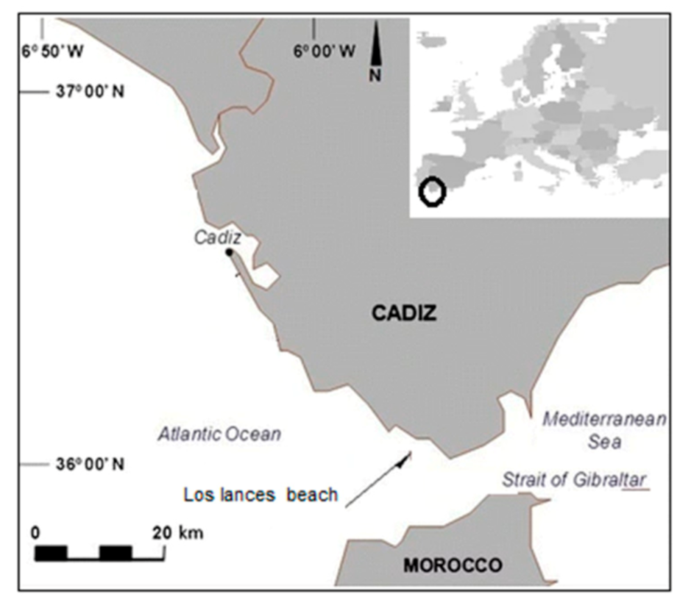
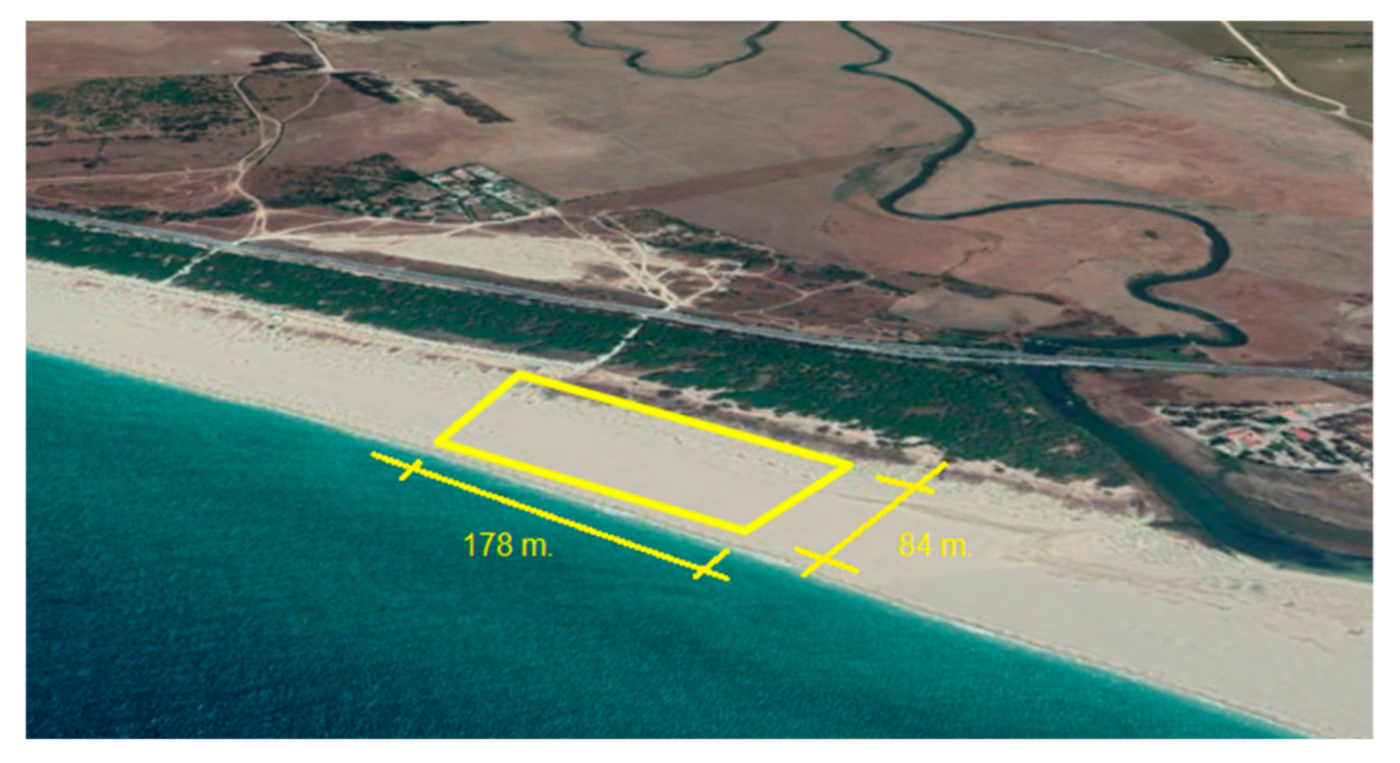
2. Study Area
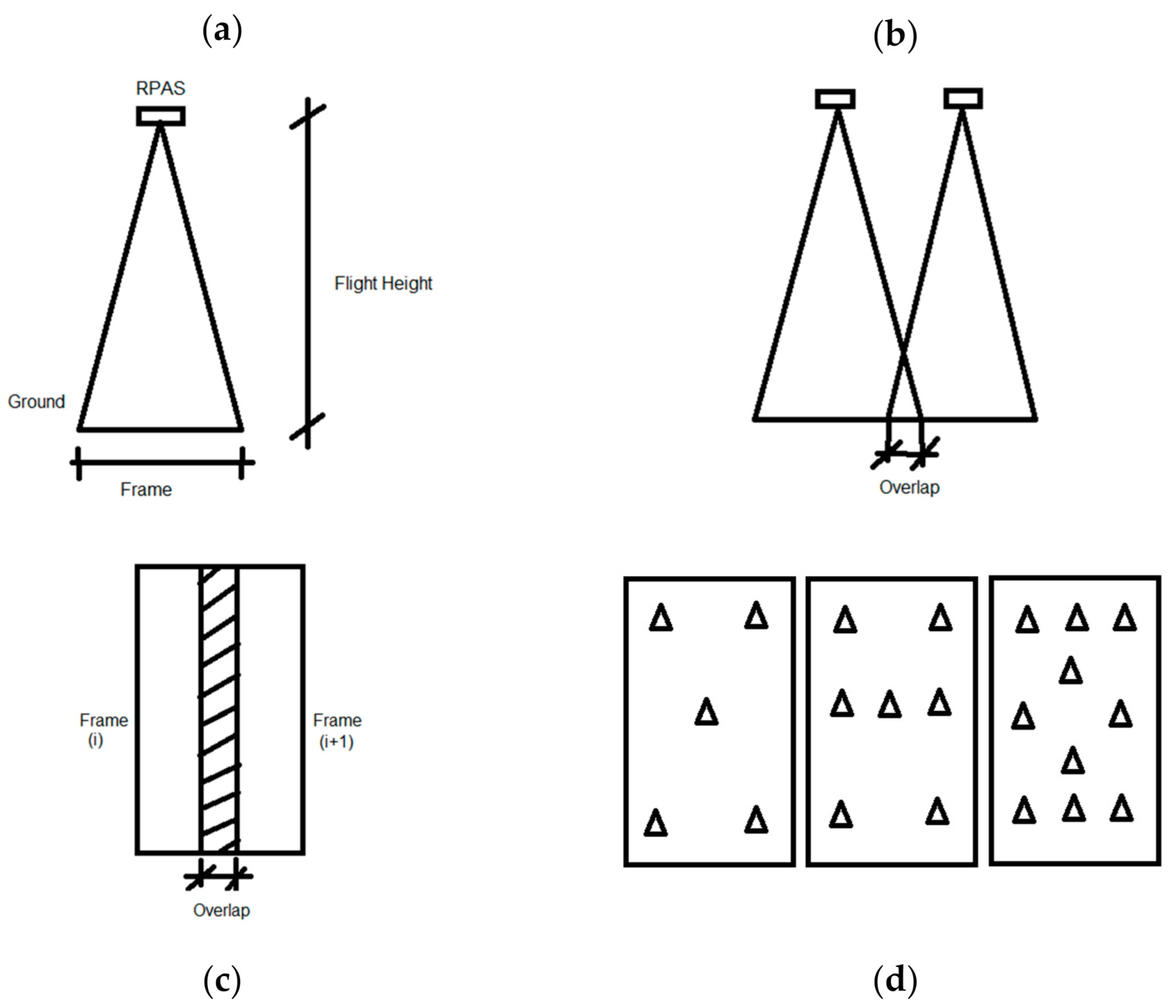
3. Methods
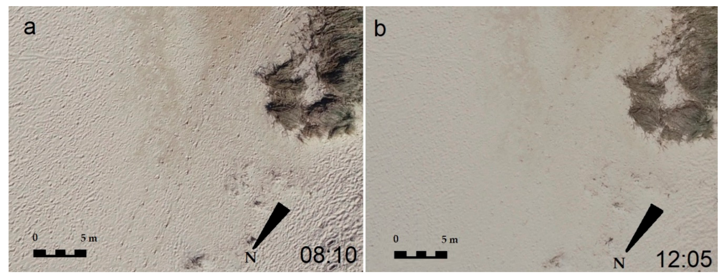
- Data collection at 8 a.m. and 12 p.m.,
- Flight height at 60, 80, and 100 m,
- Side overlap at 85% and 70%,
- Forward overlap at 85% and 70%,
- Number of GCPs on each flight: 10, 7, and 5.
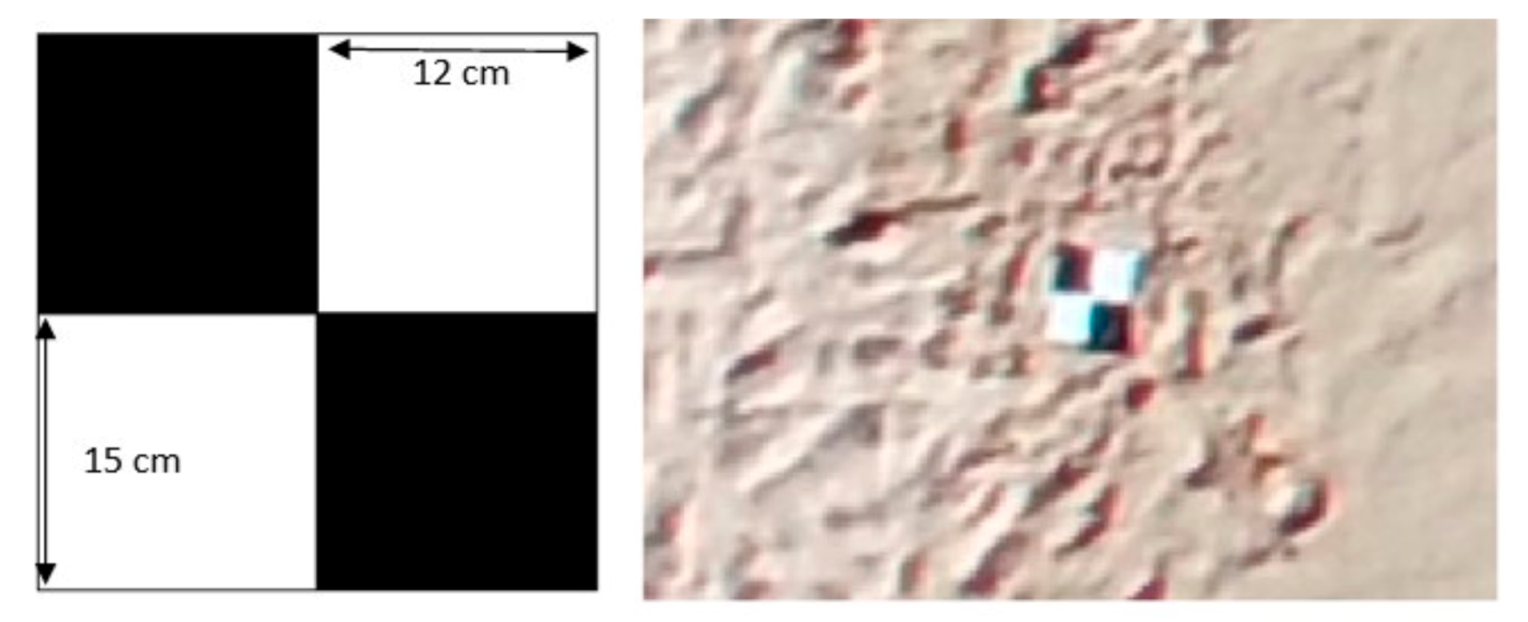
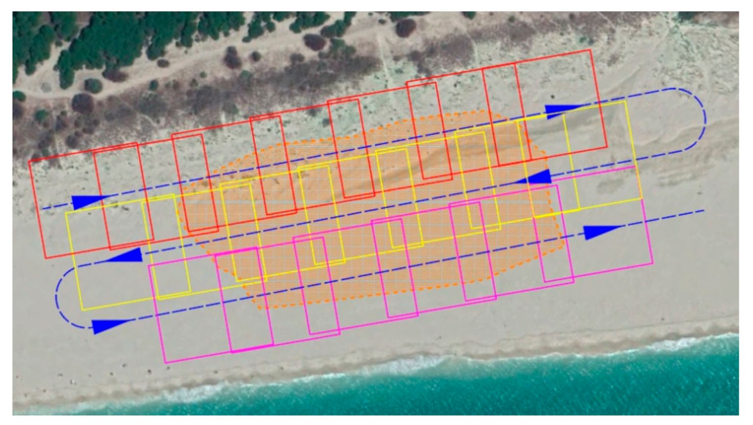
3.1. Data Collection
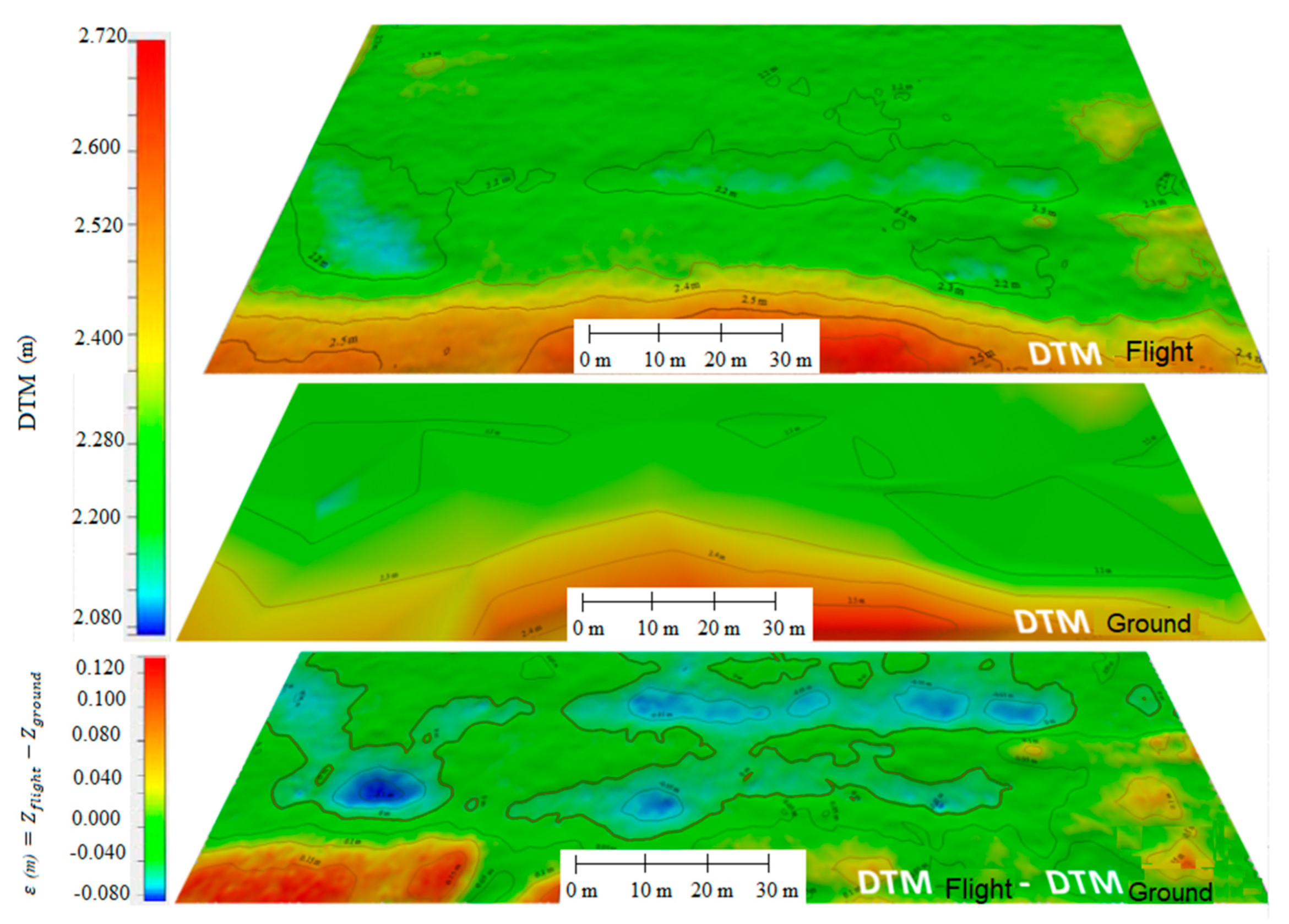
3.2. Method of Obtaining DTM by Photogrammetry and DTM Checking
3.3. Calculation of the Error
4. Results and Discussion
4.1. Error for Each of the 72 Cases
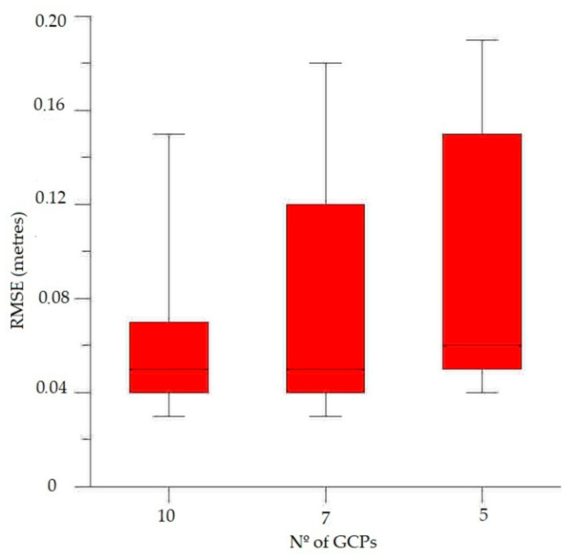
4.2. Influence of Number of GCPs
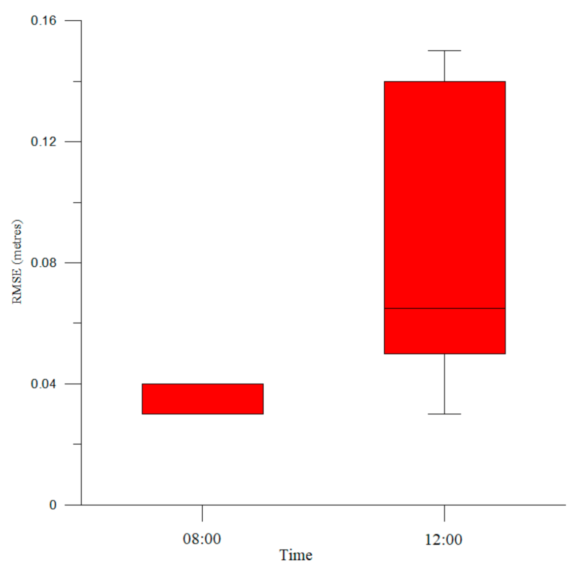
4.3. Influence of Flight Time
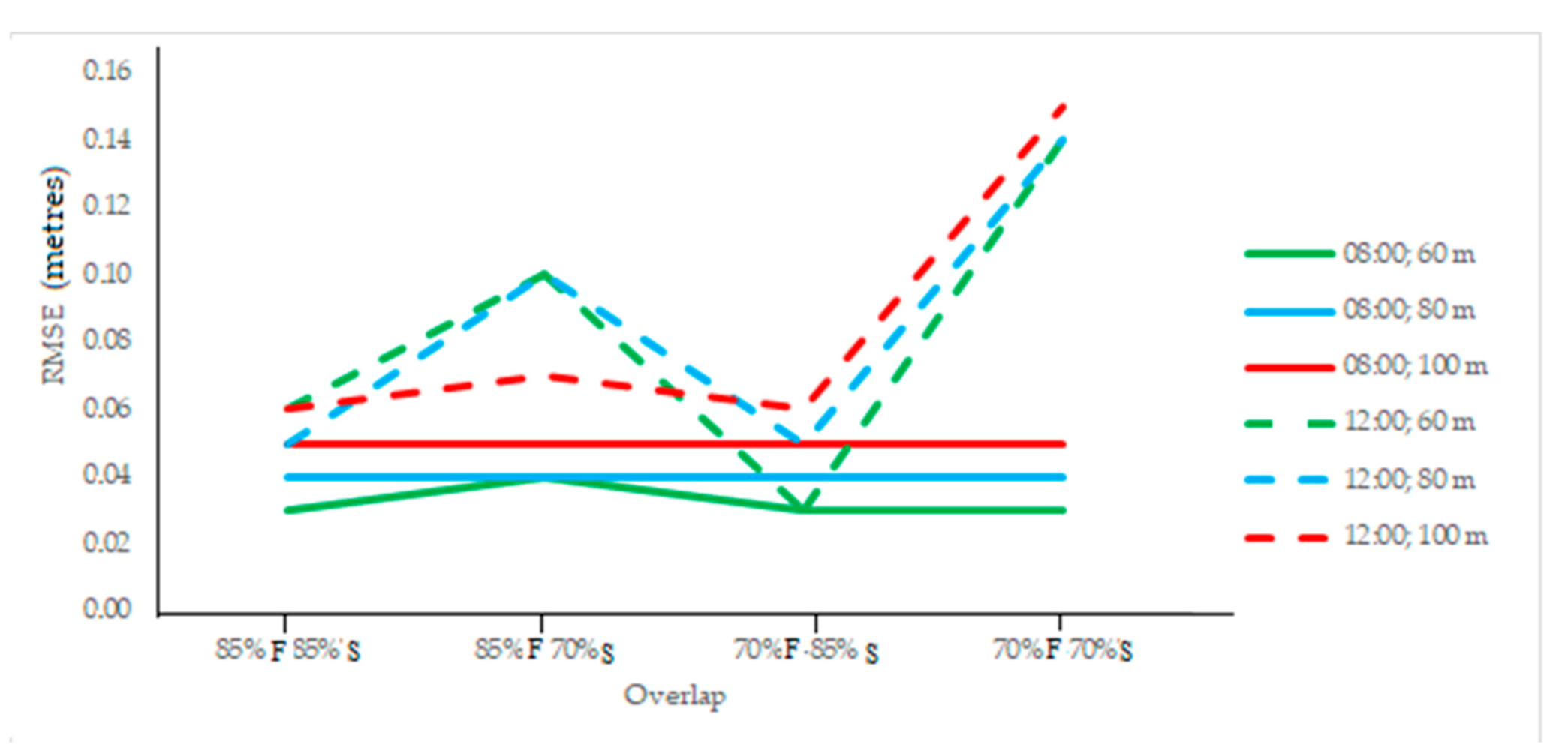
4.4. Influence of Frame Overlap and Flight Height
5. Conclusions
Author Contributions
Funding
Informed Consent Statement
Data Availability Statement
Conflicts of Interest
References
- Muñoz-Perez, J.J.; Medina, R. Comparison of long-, medium- and short-term variations of beach profiles with and without submerged geological control. Coast. Eng. 2010, 57, 241–251. [Google Scholar] [CrossRef]
- Houston, J. International tourism and US beaches. ShoreBeach. Shore Beach 1996, 64, 3–4. [Google Scholar]
- Jigena, B.; de Gil, A.; Walliser, J.; Vidal, J.; Muñoz-Perez, J.J.; Pozo, L.; Lebrato, J. Improving the Learning Process in the Subject of Basic Maritime Training Using Gps and Google Earth As Useful Tools. INTED Proc. 2016, 1, 6161–6171. [Google Scholar] [CrossRef] [Green Version]
- Berrocoso, M.; Páez, R.; Jigena, B.; Cartula, C. The RAP Net: A Geodetic Positioning Network for Andalusia (South Spain). In Proceedings of the EUREF Publication No. 16, Mitteilungen des Bundesamtes für Kartographie und Geodäsie, Riga, Latvia, 14–16 June 2006; pp. 364–368. [Google Scholar]
- Payo, A.; Favis-Mortlock, D.; Dickson, M.; Hall, J.W.; Hurst, M.D.; Walkden, M.J.; Townend, I.; Ives, M.C.; Nicholls, R.J.; Ellis, M.A. Coastal Modelling Environment version 1.0: A framework for integrating landform-specific component models in order to simulate decadal to centennial morphological changes on complex coasts. Geosci. Model Dev. 2017, 10, 2715–2740. [Google Scholar] [CrossRef] [Green Version]
- Burdziakowski, P.; Specht, C.; Dabrowski, P.S.; Specht, M.; Lewicka, O.; Makar, A. Using UAV photogrammetry to analyse changes in the coastal zone based on the sopot tombolo (Salient) measurement project. Sensors (Switzerland) 2020, 20, 4000. [Google Scholar] [CrossRef] [PubMed]
- Contreras de Villar, A.; Gómez-Pina, G.; Muñoz-Pérez, J.J.; Contreras, F.; López-García, P.; Ruiz-Ortiz, V. New design parameters for biparabolic beach profiles (SW Cadiz, Spain). Rev. Constr. 2019, 18, 432–444. [Google Scholar] [CrossRef] [Green Version]
- Specht, C.; Lewicka, O.; Specht, M.; Dabrowski, P.; Burdziakowski, P. Methodology for carrying out measurements of the tombolo geomorphic landform using unmanned aerial and surface vehicles near Sopot Pier, Poland. J. Mar. Sci. Eng. 2020, 8, 384. [Google Scholar] [CrossRef]
- Valderrama, L.; Dubois, R.M.; Ressl, R.; Silva, R.; Cruz, C.; Muñoz-Pérez, J. Dynamics of coastline changes in Mexico. J. Geogr. Sci. 2019, 1–18. [Google Scholar] [CrossRef] [Green Version]
- Muñoz-Perez, J.J.; Payo, A.; Roman-Sierra, J.; Navarro, M.; Moreno, L. Optimization of beach profile spacing: An applicable tool for coastal monitoring. Sci. Mar. 2012, 76, 791–798. [Google Scholar] [CrossRef] [Green Version]
- Castelle, B.; Laporte-Fauret, Q.; Marieu, V.; Michalet, R.; Rosebery, D.; Bujan, S.; Lubac, B.; Bernard, J.B.; Valance, A.; Dupont, P.; et al. Nature-based solution along high-energy eroding sandy coasts: Preliminary tests on the reinstatement of natural dynamics in reprofiled coastal dunes. Water (Switzerland) 2019, 11, 2518. [Google Scholar] [CrossRef] [Green Version]
- Payo, A.; Kobayashi, N.; Muñoz-Pérez, J.; Yamada, F. Scarping predictability of sandy beaches in a multidirectional wave basin. Ciencias Mar. 2008, 34, 45–54. [Google Scholar] [CrossRef] [Green Version]
- Laporte-Fauret, Q.; Marieu, V.; Castelle, B.; Michalet, R.; Bujan, S.; Rosebery, D. Low-Cost UAV for high-resolution and large-scale coastal dune change monitoring using photogrammetry. J. Mar. Sci. Eng. 2019, 7, 63. [Google Scholar] [CrossRef] [Green Version]
- Ojeda, J.; Vallejo, I.; Malvarez, G.C. Morphometric evolution of the active dunes system of the Doñana National Park, Southern Spain (1977–1999). J. Coast. Res. 2005, 49, 40–45. [Google Scholar]
- Talavera, L.; del Río, L.; Benavente, J.; Barbero, L.; López-Ramírez, J.A. UAS & S f M-based approach to Monitor Overwash Dynamics and Beach Evolution in a Sandy Spit. J. Coast. Res. 2018, 85, 221–225. [Google Scholar] [CrossRef]
- Shervais, K.A.H.; Kirkpatrick, J.D. Smoothing and re-roughening processes: The geometric evolution of a single fault zone. J. Struct. Geol. 2016, 91, 130–143. [Google Scholar] [CrossRef]
- James, M.R.; Robson, S.; Smith, M.W. 3-D uncertainty-based topographic change detection with structure-from-motion photogrammetry: Precision maps for ground control and directly georeferenced surveys. Earth Surf. Process. Landf. 2017, 42, 1769–1788. [Google Scholar] [CrossRef]
- Gabara, G.; Sawicki, P. Multi-variant accuracy evaluation of UAV imaging surveys: A case study on investment area. Sensors (Switzerland) 2019, 19, 5229. [Google Scholar] [CrossRef] [Green Version]
- Fisher, P.F.; Tate, N.J. Causes and consequences of error in digital elevation models. Prog. Phys. Geogr. 2006, 30, 467–489. [Google Scholar] [CrossRef]
- Hugenholtz, C.H.; Whitehead, K.; Brown, O.W.; Barchyn, T.E.; Moorman, B.J.; LeClair, A.; Riddell, K.; Hamilton, T. Geomorphological mapping with a small unmanned aircraft system (sUAS): Feature detection and accuracy assessment of a photogrammetrically-derived digital terrain model. Geomorphology 2013, 194, 16–24. [Google Scholar] [CrossRef] [Green Version]
- Gindraux, S.; Boesch, R.; Farinotti, D. Accuracy assessment of digital surface models from Unmanned Aerial Vehicles’ imagery on glaciers. Remote Sens. 2017, 9, 186. [Google Scholar] [CrossRef] [Green Version]
- Barbero, J.J.; García-López, L.; López-Ramírez, S.; Muñoz, J.A. RPAS as a New Tool for the Study of Sand Dunes in Coastal Environments: A Case Study in the South Atlantic Area of Spain; Vila real (Portugal) 2017. Available online: http://uas4enviro2017.utad.pt/wp-content/uploads/2017/10/Abstract_Book_UAS4Enviro2017_completo.pdf (accessed on 30 October 2020).
- Li, Z.; Zhu, Q.; Gold, C. Digital Terrain Modeling Principles and Methodology, 1st ed.; CRC Press: Boca Raton, FL, USA, 2004; ISBN 9780415324625. [Google Scholar]
- Puertos del Estado. Available online: http://www.puertos.es/es-es/oceanografia/Paginas/portus.aspx (accessed on 30 October 2020).
- Hidtma, S.L.; UTE Ecoatlántico. Estudio Ecocartográfico del Litoral de la Provincia de Cádiz. Ministry of the Environment Ref. 28-4983. 2013. Available online: https://www.miteco.gob.es/es/costas/temas/proteccion-costa/ecocartografias/ecocartografia-cadiz.aspx (accessed on 30 October 2020).
- Moloney, J.G.; Hilton, M.J.; Sirguey, P.; Simons-Smith, T. Coastal Dune Surveying Using a Low-Cost Remotely Piloted Aerial System (RPAS). J. Coast. Res. 2018, 34, 1244–1255. [Google Scholar] [CrossRef]
- Taddia, Y.; Stecchi, F.; Pellegrinelli, A. Coastal Mapping Using DJI Phantom 4 RTK in Post-Processing Kinematic Mode. Drones 2020, 4, 9. [Google Scholar] [CrossRef] [Green Version]
- de Fomento, M. Instituto Geográfico Nacional. Available online: https://www.ign.es/web/ign/portal (accessed on 30 October 2020).
- Ground Sampling Distance (GSD). Available online: https://support.pix4d.com/hc/en-us/articles/202559809-Ground-sampling-distance-GSD (accessed on 29 January 2020).
- Zimmerman, T.; Jansen, K.; Miller, J. Analysis of UAS Flight Altitude and Ground Control Point Parameters on DEM Accuracy along a Complex, Developed Coastline. Remote Sens. 2020, 12, 2305. [Google Scholar] [CrossRef]
- James, M.R.; Chandler, J.H.; Eltner, A.; Fraser, C.; Miller, P.E.; Mills, J.P.; Noble, T.; Robson, S.; Lane, S.N. Guidelines on the use of structure-from-motion photogrammetry in geomorphic research. Earth Surf. Process. Landforms 2019, 44, 2081–2084. [Google Scholar] [CrossRef]
- National Standard for Spatial Data Accuracy. 1998. Available online: https://www.fgdc.gov/standards/projects/accuracy/part3/chapter3 (accessed on 30 October 2020).
- Ruiz-Lendínez, J.J.; Ariza-López, F.J.; Ureña-Cámara, M.A. Study of NSSDA variability by means of automatic positional accuracy assessment methods. ISPRS Int. J. Geo-Inf. 2019, 8, 552. [Google Scholar] [CrossRef] [Green Version]
- James, M.R.; Robson, S.; d’Oleire-Oltmanns, S.; Niethammer, U. Optimising UAV topographic surveys processed with structure-from-motion: Ground control quality, quantity and bundle adjustment. Geomorphology 2017, 280, 51–66. [Google Scholar] [CrossRef] [Green Version]
- Gonçalves, J.A.; Henriques, R. UAV photogrammetry for topographic monitoring of coastal areas. ISPRS J. Photogramm. Remote Sens. 2015, 104, 101–111. [Google Scholar] [CrossRef]


| Parameter | Values | Number of Cases |
|---|---|---|
| Flight time | 8 a.m. and 12 p.m. | 2 |
| Flight height | 60, 80, and 100 m | 3 |
| Longitudinal overlap | 70% and 85% | 2 |
| Transverse overlap | 70% and 85% | 2 |
| Number of GCPs | 5, 7, and 10 | 3 |
| Total number of cases | - | 72 |
| Sensor | 1” CMOS |
|---|---|
| Effective Pixels: 20M | |
| Lens | FOV 84° 8.8 mm/24 mm (35 mm format equivalent) f/2.8−f/11 autofocus at 1 m-∞ |
| Iso Range | Photo: |
| 100–3200 (Auto) | |
| 8–1/2000 s | |
| 8–1/8000 s | |
| Mechanical Shutter Speed | 3:2 Aspect Ratio 5472 × 3648 |
| Electronic Shutter Speed | 4:3 Aspect Ratio 4864 × 3648 |
| Image Size | 16:9 Aspect Ratio 5472 × 3078 |
| 4096 × 2160 (4096 × 2160 24/25/30/48/50p) | |
| 3840 × 2160 (3840 × 2160 24/25/30/48/50/60p) | |
| PIV Image size | 2720 × 1530 (2720 × 1530 24/25/30/48/50/60p) |
| Single Shot | |
| Burst Shooting: 3/5/7/10/14 frames | |
| Still Photography modes | Auto Exposure Bracketing (AEB): dL/5 at 0.7 |
| EV Bias Internal 2/3/5/7/10/15/20/30/60 s |
| Flight Height (m) | GSD (cm/pixel) | Frame Size (m·m) | Number of Frames | Duration of Flight (min) |
|---|---|---|---|---|
| 60 | 1.64 | 90 × 60 | 185 | 16 |
| 80 | 2.18 | 119 × 80 | 123 | 11 |
| 100 | 2.73 | 148 × 98 | 81 | 9 |
| Flight Time | Flight Height (m) | Type of Error | Overlap | |||||||||||
|---|---|---|---|---|---|---|---|---|---|---|---|---|---|---|
| 85%F−85%S | 85%F−70%S | 70%F−85%S | 70%F−70%S | |||||||||||
| Number of GCPs | ||||||||||||||
| 10 | 7 GCP | 5 GCP | 10 GCP | 7 GCP | 5 GCP | 10 GCP | 7 GCP | 5 GCP | 10 GCP | 7 GCP | 5 GCP | |||
| 8 a.m. | 60 | RMSE (m) | 0.03 | 0.05 | 0.05 | 0.04 | 0.04 | 0.05 | 0.03 | 0.06 | 0.05 | 0.03 | 0.03 | 0.05 |
| Vertical accuracy (1.96·RMSE) | 0.06 | 0.10 | 0.10 | 0.08 | 0.08 | 0.10 | 0.06 | 0.12 | 0.10 | 0.06 | 0.06 | 0.10 | ||
| % grid with data | 65.80% | 59.73% | 59.73% | 60.29% | ||||||||||
| 80 | RMSE (m) | 0.04 | 0.04 | 0.04 | 0.04 | 0.04 | 0.04 | 0.04 | 0.04 | 0.04 | 0.04 | 0.04 | 0.05 | |
| Vertical accuracy (1.96·RMSE) | 0.08 | 0.08 | 0.08 | 0.08 | 0.08 | 0.08 | 0.08 | 0.08 | 0.08 | 0.08 | 0.08 | 0.10 | ||
| % grid with data | 60.45% | 60.15% | 60.85% | 55.83% | ||||||||||
| 100 | RMSE (m) | 0.05 | 0.07 | 0.09 | 0.05 | 0.05 | 0.09 | 0.05 | 0.05 | 0.08 | 0.05 | 0.05 | 0.19 | |
| Vertical accuracy (1.96·RMSE) | 0.10 | 0.14 | 0.18 | 0.10 | 0.10 | 0.18 | 0.10 | 0.10 | 0.16 | 0.10 | 0.10 | 0.37 | ||
| % grid with data | 46.00% | 36.00% | 36.00% | 35.97% | ||||||||||
| 12 p.m. | 60 | RMSE (m) | 0.06 | 0.05 | 0.05 | 0.10 | 0.14 | 0.15 | 0.033 | 0.04 | 0.04 | 0.14 | 0.15 | 0.16 |
| Vertical accuracy (1.96·RMSE) | 0.12 | 0.10 | 0.10 | 0.20 | 0.27 | 0.29 | 0.06 | 0.08 | 0.08 | 0.27 | 0.29 | 0.31 | ||
| % grid with data | 43.24% | 39.26% | 37.60% | 38.53% | ||||||||||
| 80 | RMSE (m) | 0.05 | 0.05 | 0.05 | 0.10 | 0.14 | 0.16 | 0.05 | 0.05 | 0.05 | 0.145 | 0.17 | 0.17 | |
| Vertical accuracy (1.96·RMSE) | 0.10 | 0.10 | 0.10 | 0.20 | 0.27 | 0.31 | 0.10 | 0.10 | 0.10 | 0.27 | 0.33 | 0.33 | ||
| % grid with data | 39.03% | 36.17% | 36.95% | 33.47% | ||||||||||
| 100 | RMSE (m) | 0.06 | 0.12 | 0.13 | 0.07 | 0.04 | 0.09 | 0.06 | 0.07 | 0.07 | 0.15 | 0.18 | 0.19 | |
| Vertical accuracy (1.96·RMSE) | 0.12 | 0.24 | 0.25 | 0.14 | 0.08 | 0.18 | 0.12 | 0.14 | 0.14 | 0.29 | 0.355 | 0.37 | ||
| % grid with data | 29.66% | 20.47% | 21.37% | 19.18% | ||||||||||
| Flight Time | Flight Height | Number of Tie Points |
|---|---|---|
| 60 m | 105,382 | |
| 08:00 a.m. | 80 m | 76,852 |
| 100 m | 32,733 | |
| 60 m | 39,296 | |
| 12:00 a.m. | 80 m | 29,639 |
| 100 m | 19,848 |
Publisher’s Note: MDPI stays neutral with regard to jurisdictional claims in published maps and institutional affiliations. |
© 2020 by the authors. Licensee MDPI, Basel, Switzerland. This article is an open access article distributed under the terms and conditions of the Creative Commons Attribution (CC BY) license (http://creativecommons.org/licenses/by/4.0/).
Share and Cite
Contreras-de-Villar, F.; García, F.J.; Muñoz-Perez, J.J.; Contreras-de-Villar, A.; Ruiz-Ortiz, V.; Lopez, P.; Garcia-López, S.; Jigena, B. Beach Leveling Using a Remotely Piloted Aircraft System (RPAS): Problems and Solutions. J. Mar. Sci. Eng. 2021, 9, 19. https://doi.org/10.3390/jmse9010019
Contreras-de-Villar F, García FJ, Muñoz-Perez JJ, Contreras-de-Villar A, Ruiz-Ortiz V, Lopez P, Garcia-López S, Jigena B. Beach Leveling Using a Remotely Piloted Aircraft System (RPAS): Problems and Solutions. Journal of Marine Science and Engineering. 2021; 9(1):19. https://doi.org/10.3390/jmse9010019
Chicago/Turabian StyleContreras-de-Villar, Francisco, Francisco J. García, Juan J. Muñoz-Perez, Antonio Contreras-de-Villar, Veronica Ruiz-Ortiz, Patricia Lopez, Santiago Garcia-López, and Bismarck Jigena. 2021. "Beach Leveling Using a Remotely Piloted Aircraft System (RPAS): Problems and Solutions" Journal of Marine Science and Engineering 9, no. 1: 19. https://doi.org/10.3390/jmse9010019