On the Sensitivity of Typhoon Wave Simulations to Tidal Elevation and Current

Abstract

The sensitivity of storm wave simulations to storm tides and tidal currents was investigated using a high-resolution, unstructured-grid, coupled circulation-wave model (Semi-implicit Cross-scale Hydroscience Integrated System Model Wind Wave Model version III (SCHISM-WWM-III)) driven by two typhoon events (Typhoons Soudelor and Megi) impacting the northeastern coast of Taiwan. Hourly wind fields were acquired from a fifth-generation global atmospheric reanalysis (ERA5) and were used as meteorological conditions for the circulation-wave model after direct modification (MERA5). The large typhoon-induced waves derived from SCHISM-WWM-III were significantly improved with the MERA5 winds, and the peak wave height was increased by 1.0–2.0 m. A series of numerical experiments were conducted with SCHISM-WWM-II and MERA5 to explore the responses of typhoon wave simulations to tidal elevation and current. The results demonstrate that the simulated significant wave height, mean wave period and wave direction for a wave buoy in the outer region of the typhoon are more sensitive to the tidal current but less sensitive to the tidal elevation than those for a wave buoy moored in the inner region of the typhoon. This study suggests that the inclusion of the tidal current and elevation could be more important for typhoon wave modeling in sea areas with larger tidal ranges and higher tidal currents. Additionally, the suitable modification of the typhoon winds from a global atmospheric reanalysis is necessary for the accurate simulation of storm waves over the entire region of a typhoon.

1. Introduction

Extreme waves and storm surges resulting from typhoons are usually regarded as destructive disasters that present a great hazard to navigational safety and coastal and nearshore infrastructures and can flood low-lying areas along the coast [1,2,3]. To mitigate the disaster risk in both nearshore and coastal regions, many researchers have put considerable effort into the improvement of storm wave and storm surge modeling [2,3,4]. To achieve this goal, it is important to enhance the predictive capabilities of the typhoon storm surge and wave models used for emergency preparedness and risk evaluation. In addition, the ability to accurately predict large-wave events is critical to the success of wave energy conversion deployment [5].

Research on the nonlinear interactions between the tidal current, tidal elevation, and waves is complex because such studies require an understanding of the corresponding transfer mechanisms. The performance of typhoon storm surge and wave models strongly depends on a complete understanding of these physical processes. Longuet-Higgins and Stewart [6] and Phillips [7] clarified the transfer of momentum from ocean surface waves to tidal currents. The momentum flux between wind and current is based on the wind stress bulk formula and is proportional to the square of the wind speed [8]. The radiation stress theory proposed in Reference [6] provides an approach for introducing wave-induced forces into tidal currents. The contributions of waves to a storm surge or storm tide through radiation-stress-induced forces can be examined by coupling a circulation model with a wave model [9,10]. However, further clarification is needed to capture the contributions of the tidal current and tidal elevation to storm waves. Huang et al. [9] analyzed the effects of a storm surge on waves by comparing wave simulations with and without a storm surge for Tampa Bay in Florida. The results of their study indicated that the simulated significant wave heights could be increased by 1.0–1.5 m, and the simulated peak wave height could see perhaps as much as a 2–3 m increase. They found that the contribution of the storm surge to the significant wave height was greater than that of the significant wave height to the storm surge. This is because the Tampa Bay region is close to a gently sloping continental shelf, which allows the wind stress to be more influential than the wave-induced force in generating a storm surge. Although Huang et al. [9] investigated the storm surge effect on waves, the current understanding of the contributions of the tide and tidal current to waves is still lacking. A comprehensive understanding of the interactions between storm waves, tidal current, and tidal elevation would be of great interest to coastal and ocean engineers and oceanographers.

Rusu et al. [11] and Van Vledder and Akpınar [12] suggested that model predictions of wave fields could be greatly improved if winds of a higher spatial resolution were used in the numerical model. Rusu et al. [11] also noted that wind fields with a spatial resolution of 4.1 km are satisfactory for wind wave modeling. However, considerable computational resources and a long model execution time are required. In contrast, a simple method was applied in the present study to improve the typhoon winds acquired from a reanalysis product.

The goal of the present study was to investigate the sensitivity of storm wave simulations to tidal currents and tidal elevations during two typhoons impacting Taiwan in 2015 and 2016 by means of a series of model experiments. This paper is organized as follows. The studied typhoons, the data recorded at the wave buoys, the circulation and wave models, the bathymetry, the typhoon winds, and the boundary conditions that were used in the present study are described in Section 2. In Section 3, the significant wave height time series are compared among several different simulation scenarios. A discussion of the results from the series of model experiments and a confirmation of the results are provided in Section 4, and a summary and conclusions are offered in Section 5.

2. Data and Models

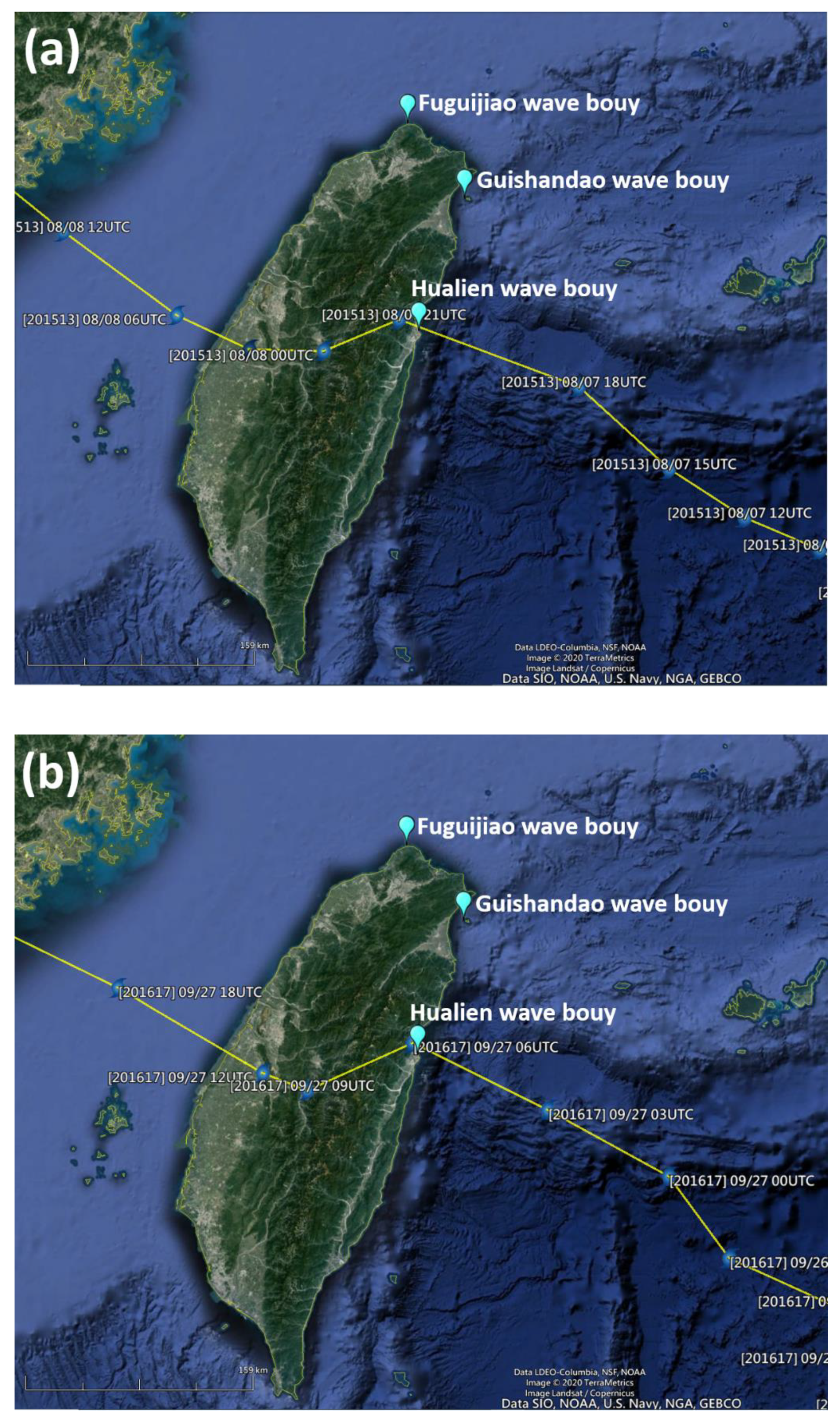
2.1. Description of the Studied Typhoons

Typhoon Soudelor, also known as Typhoon Hanna in the Philippines, was the strongest tropical cyclone of the 2015 Pacific typhoon season and the third most intense tropical cyclone worldwide in 2015. Soudelor formed as a tropical depression in the southeastern sea area of Guam on 29 July and reached its peak intensity, with a central atmospheric pressure of 900 hPa and ten-minute maximum sustained winds of 215 km/h, on 3 August. Soudelor was a Category 5-equivalent super typhoon, according to a wind speed assessment by the Joint Typhoon Warning Center (JTWC). Soudelor, which made landfall over Hualien County of Taiwan on 7 August and emerged in the Taiwan Strait early the next day, had a severe impact on Taiwan.

Typhoon Megi was a large and powerful tropical cyclone that hit Taiwan and southeastern China in late September 2016. The Japan Meteorological Agency (JMA) indicated that Typhoon Megi had reached its peak intensity at 18:00 UTC on 26 September, with ten-minute maximum sustained winds of 155 km/h and a central pressure of 940 hPa. However, Typhoon Megi had already intensified into a stronger typhoon at approximately 03:00 UTC on 27 September, with one-minute maximum sustained winds of 220 km/h (equivalent to Category 4 on the Saffir–Simpson hurricane wind scale), before it made landfall over Hualien County at 06:00 UTC. Megi emerged into the Taiwan Strait from Yunlin County at 13:10 UTC and subsequently made landfall over Fujian Province of China at 20:40 UTC on 27 September as a weaker typhoon. The tracks, central positions, and arrival times of Typhoons Soudelor and Megi were acquired from the best track data of the Regional Specialized Meteorological Center (RSMC) Tokyo-Typhoon Center, and are illustrated in Figure 1 (Figure 1a for Typhoon Soudelor and Figure 1b for Typhoon Megi).

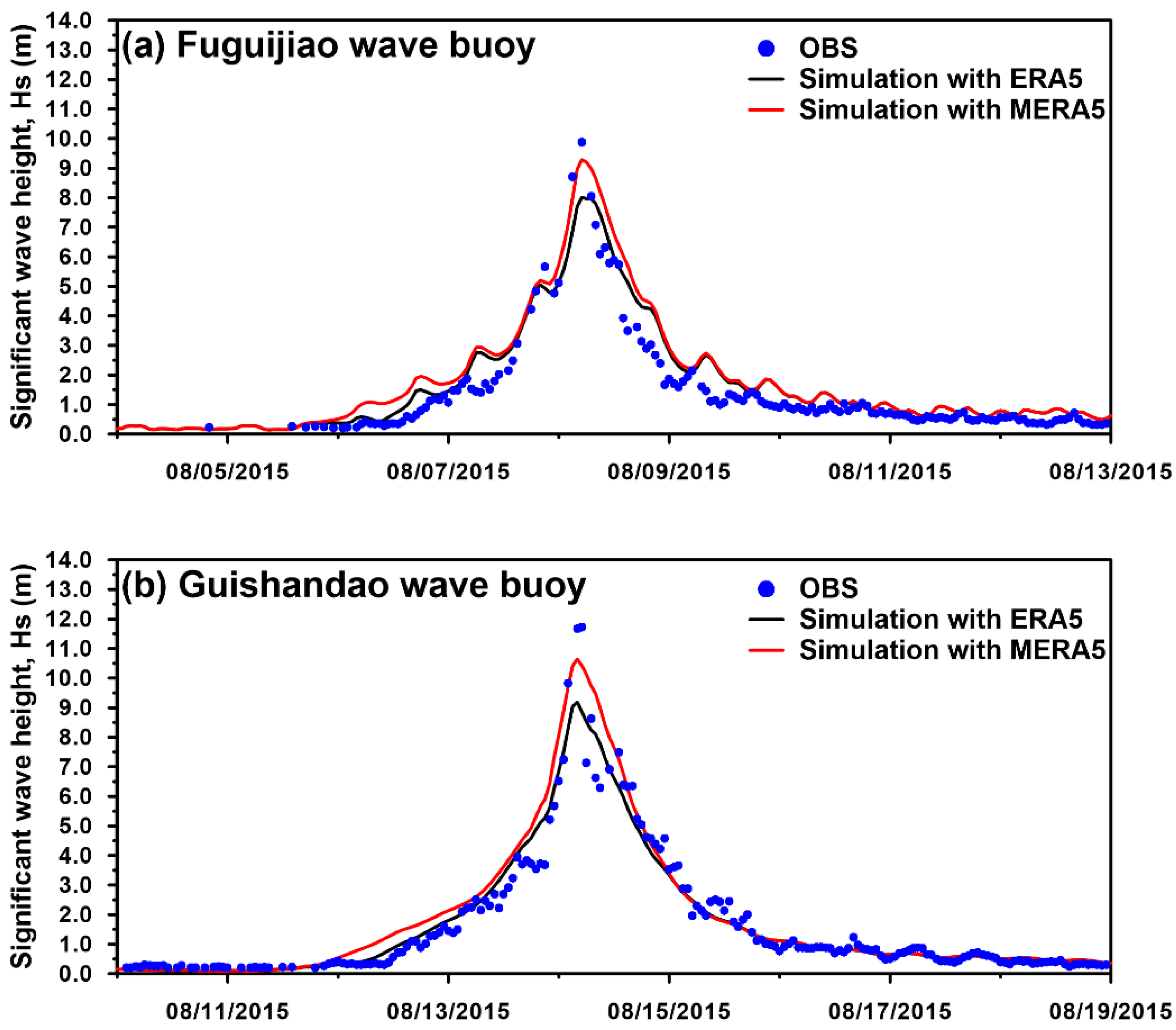
2.2. Description of the Adopted Wave Buoys

The Central Weather Bureau (CWB) of Taiwan has deployed many wave buoys in the nearshore waters for long-term monitoring of wave parameters. In this study, the significant wave height (Hs), mean wave period (Tm), and wave direction (WD) data measured at three wave buoys in the northeastern waters of Taiwan during Typhoon Soudelor in 2015 and Typhoon Megi in 2016 were applied to evaluate the Hs simulation performance achieved with a high-resolution coupled circulation-wave model. According to the buoy observation dada annual report from the CWB, the sampling frequency of wave buoys is 2 Hz for 10 min in the beginning of each hour. The recorded acceleration time series is transferred to acceleration spectrum and then converted to the one-dimensional wave spectrum. The zeroth (m₀) and second (m₂) moments of the wave power spectrum can be obtained by integrating the one-dimensional wave spectrum. Finally, the significant wave height and mean wave period are calculated as: Hs = 4.004√m₀ and Tm = √(m₀/m₂). The wave direction is the direction of the most energetic wave in the spectrum. The buoy names and locations are shown in Figure 1, and the coordinates and water depths of their deployment sites are listed in

Table 1. Information on the adopted wave buoys.

Buoy Name	Longitude (°E)	Latitude (°N)	Water Depth (m)
Fuguijiao	121.535	25.3042	34
Guishandao	121.9261	24.8467	25
Hualien	121.6325	24.03111	22

Data source: The Central Weather Bureau (CWB) of Taiwan.

.

2.3. Barotropic 2-D Ocean Circulation Model

The Semi-implicit Cross-scale Hydroscience Integrated System Model (SCHISM) was employed to simulate the storm tidal elevations and tidal currents in the waters surrounding Taiwan during Typhoons Soudelor and Megi. In SCHISM, the primitive shallow-water equation is solved on an unstructured grid using finite-element and finite-volume methods based on the hydrostatic and Boussinesq approximations [13]. With many new corrections and upgrades from the Semi-implicit Eulerian-Lagrangian Finite-Element (SELFE) model [14], SCHISM now has an open-source distribution that is licensed under the Apache License Version 2.0. The numerical stability constraints are relaxed due to the application of the semi-implicit scheme in SCHISM. SCHISM and SELFE have been used in the simulation of storm surge inundation [15,16,17] and riverine flash flooding [18], in the evaluation of tidal current energy variations resulting from sea-level rise [19], and in investigation of fecal coliform transportation in an estuarine system [20]. A two-dimensional model is preferred over a three-dimensional model for storm surge, storm tide, and wind wave modeling because two-dimensional models require less execution time and computational resource consumption; therefore, SCHISM-2D, a depth-integrated version of SCHISM, was utilized in the present study to simulate the sea-surface elevations and currents. The governing equations in two-dimensional form are written in the Cartesian coordinate system as follows:

$$\frac{\partial \eta }{\partial t}+\frac{\partial uH}{\partial x}+\frac{\partial vH}{\partial y}=0,$$

(1)

$$\frac{Du}{Dt}=fv-\frac{\partial }{\partial x}\left\{g(\eta -\alpha \widehat{\psi })+\frac{P_A}{{\rho }_0}\right\}+\frac{{\tau }_{sx}+{\tau }_{rx}-{\tau }_{bx}}{{\rho }_{0}H},$$

(2)

$$\frac{Dv}{Dt}=-fu-\frac{\partial }{\partial y}\left\{g(\eta -\alpha \widehat{\psi })+\frac{P_A}{{\rho }_0}\right\}+\frac{{\tau }_{sy}+{\tau }_{ry}-{\tau }_{by}}{{\rho }_{0}H},$$

(3)

where D is the material derivative, t is the time, η(x,y,t) is the free-surface elevation, u(x,y,t) and ν(x,y,t) are the horizontal velocities, h is the seafloor elevation, H = η + h is the total water depth, f is the Coriolis factor, g is the gravitational acceleration, $\widehat{\psi }$ is the Earth’s tidal potential, α is the effective Earth elasticity factor, ρ₀ is the reference water density, and P_A(x,y,t) is the sea-surface atmospheric pressure. τ_sx and τ_sy are the wind stresses, which can be expressed as:

$${\tau }_{sx}={\rho }_a{C}_s\sqrt{{W_x}^2+{W_y}^2}{W}_x,$$

(4)

$${\tau }_{sy}={\rho }_a{C}_s\sqrt{{W_x}^2+{W_y}^2}{W}_y,$$

(5)

where ρ_a is the air density, C_s is the wind drag coefficient, and W_x and W_y are the wind speeds at 10 m above the sea surface. Powell et al. [21] suggested that an upper bound on C_s is necessary in the model in the case of high wind speeds; thus, SCHISM-2D calculates C_s following the formula proposed by Smith [22] but with an embedded cap for cases in which the wind speed exceeds a specific value:

$$C_s={1.0}^{-3}\{\begin{array}{cc}0.61+0.063\times 6.0,\hfill & \hfill W<6.0\hfill \\ 0.61+0.063\times W,\hfill & \hfill 6.0\le W\le 50.0\hfill \\ 0.61+0.063\times 50.0,\hfill & \hfill W>50.0\hfill \end{array},$$

(6)

where W is the resultant wind speed.

τ_bx and τ_by in Equations (2) and (3) are the bottom shear stresses, which can be computed as:

$${\tau }_{bx}={\rho }_0{C}_d\sqrt{u^2+v^2}u,$$

(7)

$${\tau }_{by}={\rho }_0{C}_d\sqrt{u^2+v^2}v,$$

(8)

where C_d is the bottom drag coefficient, which is parameterized as follows:

$$C_d=g{n}^2/H^{1/3},$$

(9)

where n is the Manning coefficient. Equation (2) indicates that the bottom drag coefficient C_d varies spatially with different values of H. In Equations (2) and (3), τ_rx and τ_ry are the radiation stresses, which are computed using a wind wave model as reported by Longuet-Higgins and Stewart [6,23].

2.4. Ocean Surface Wave Model

Komen [24] suggested that the ocean surface waves induced by wind can be simulated through phase-averaged spectral wave models. Therefore, a third-generation spectral wave model, the Wind Wave Model version III (WWM-III), was utilized in the present study to model typhoon-generated extreme sea states in Taiwanese waters. Roland [25] overhauled the original WWM-I source code from Hsu et al. [26] and upgraded it to WWM-II. Comparisons between WWM-II and the Simulating WAves Nearshore (SWAN) model, developed by Booij et al. [27], for test cases of continental shelf refraction showed that the Residual Distribution Flux Corrected Transport scheme implemented in WWM-II is able to accurately resolve the directional spreading over a continental shelf profile and that the resulting simulations are far superior to those using the SWAN model with a higher-order scheme at the same mesh resolution. WWM-III is the latest version of WWM, with many enhancements and improvements, and has already been applied to reproduce the long-term wave parameters in the nearshore waters of Taiwan [28]. In WWM-III, the governing wave action balance equation is solved on an unstructured grid:

$$\frac{\partial N}{\partial t}+\frac{\partial (C_{gx}+u)N}{\partial x}+\frac{\partial (C_{gy}+v)N}{\partial y}+\frac{\partial (C_{\sigma }N)}{\partial \sigma }+\frac{\partial (C_{\theta }N)}{\partial \theta }=\frac{S_{tot}}{\sigma },$$

(10)

where N(σ, θ) is the spectral wave action density, C_gx and C_gy are the wave group velocities in the x and y directions, and C_σ and C_θ are the propagation velocities in spectral space (σ, θ). S_tot is the sum of the source terms for wave variance, which can be defined as:

$$S_{tot}=S_{in}+S_{wc}+S_{nl4}+S_{nl3}+S_{br}+S_{bf},$$

(11)

where S_in is the wind-induced energy input; S_nl3 and S_nl4 are the nonlinear interactions in shallow and deep-water areas, respectively; S_wc and S_br represent the wave energy dissipation in deep- and shallow-water areas caused by white capping and wave breaking, respectively; and S_bf is the dissipation caused by bottom friction. The first three source terms in Equation (11) are significant in deep water, while the last three terms are influential in shallow water. A peak enhancement of 3.3 and a bottom friction factor of 0.067 have been specified in WWM-III following a report from the Joint North Sea Wave Project (JONSWAP, Hasselmann et al. [29]). A wave-breaking coefficient of 0.78 is adopted for computing wave breaking in WWM-III. Nonlinear wave-wave interactions are treated with the discrete interaction approximation (DIA) proposed by Hasselmann et al. [30]. The wave direction is equally discretized into 36 bins over a range of 0–360°. The number of frequency bins is also 36, and the low- and high-frequency limits of the discrete wave period in WWM-III are 0.04 Hz and 1.0 Hz, respectively.

2.5. Fully Coupled SCHISM-WWM-III Model

SCHISM-2D and WWM-III take advantage of sharing the same subdomains and parallelization via the same domain decomposition scheme to eliminate interpolation errors and enhance the efficiency of information exchange between the ocean circulation and wind wave models. The computational performance of the coupled model, SCHISM-WWM-III, can be made more efficient through the use of different time steps in the two models; thus, time steps of 120 s and 600 s were assigned to the SCHISM and WWM-III models, respectively. This means that, each time information exchange is conducted between the two models, five time intervals of SCHISM-2D will have been calculated. The depth-averaged tidal current and tidal elevation are passed to WWM-III from SCHISM-2D, while WWM-III sends the radiation stresses to SCHISM-2D. The SCHISM-WWM-III modeling system has been successfully applied to hindcast, simulate, and predict storm surge and storm wave hazards and to evaluate the wave power energy in Taiwanese waters [2,3]. Further details about the coupling approaches used in SCHISM-WWM-III can be found in Reference [31].

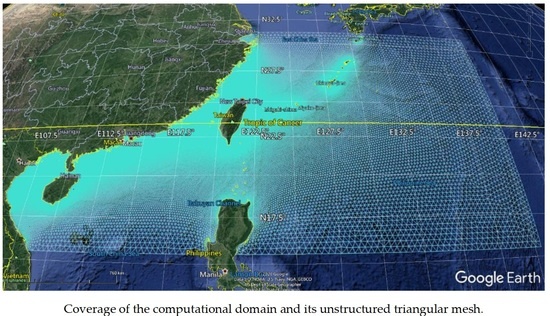
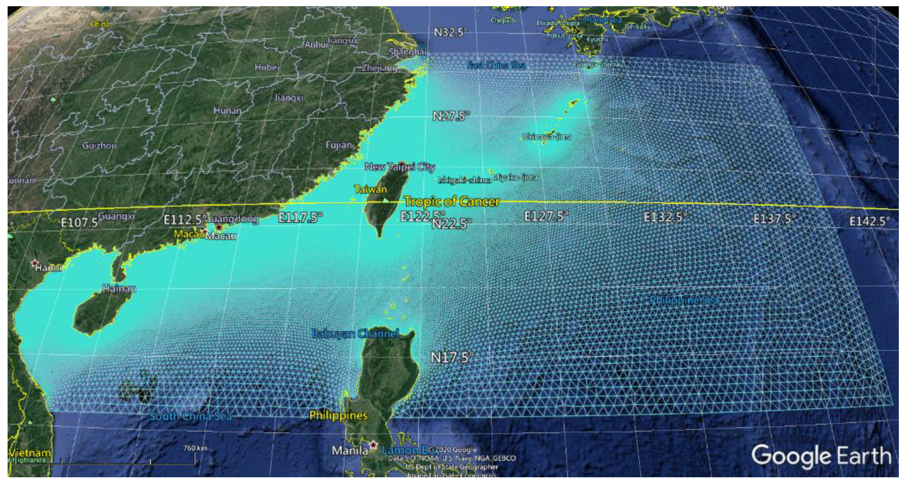
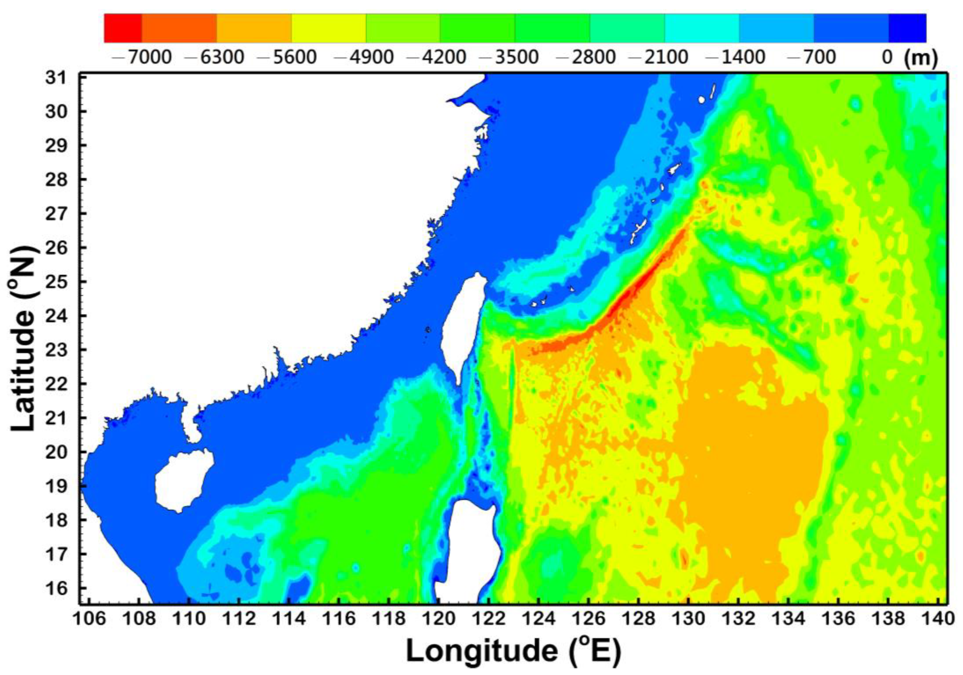
2.6. Computational Domain and Unstructured Grid

Satisfying all requirements of the model domain and mesh is essential for successful typhoon wave and storm surge modeling. An appropriate computational domain size must be large enough to accommodate the entire typhoon while minimizing the effects of boundary conditions [32,33]. Additionally, the resolution of the model mesh must be high enough to resolve the geometric details of the surf zones and shallow-water regions [34,35,36]. Figure 2 shows the coverage of the model domain specified for application to Typhoons Soudelor and Megi. The full computational extent of the SCHISM-WWM-III computational domain is from 105° E to 140° E and from 15° N to 31° N, and it comprises 276,639 unstructured grid points and 540,510 nonoverlapping triangles. The mesh is coarser in the open ocean beyond the nearshore region, with a resolution of 20–40 km. For the coastal areas of Taiwan and its offshore islands, a finer mesh with a resolution of 200–400 m is employed (as shown in Figure 2).

The gridded bathymetric data used in SCHISM-WWM-III are composed of a global-scale dataset and a local-scale dataset. The GEBCO_2019 product released in March 2019 by the General Bathymetric Chart of the Oceans (GEBCO) provides global coverage on a 15 arc-second grid. The local-scale dataset, with a spatial resolution of 200 m, was acquired from the Department of Land Administration and the Ministry of the Interior, Taiwan, and covers the area from 100° E to 128° E and from 4° N to 29° N. Figure 3 illustrates the seafloor elevations used in SCHISM-WWM-III, which were interpolated by combining the two datasets mentioned above.

2.7. Boundary Conditions

2.7.1. ERA5 Reanalysis Wind Forcing

ERA5 is the latest global climate atmospheric reanalysis released by the European Centre for Medium-Range Weather Forecasts (ECMWF). Compared to the ERA-Interim product, ERA5 has many improvements, e.g., much higher temporal and spatial resolutions, much improved tropospheric data, a better global balance between precipitation and evaporation, better precipitation over land in the deep tropics, and an improved representation of tropical cyclones, the last of which is the most important for simulating typhoon-generated waves. The hourly ERA5 atmospheric parameters, such as the wind at 10 m above the sea surface and the sea-level pressure, can be downloaded from the website of the Climate Data Store and have a spatial resolution of 30 km in the horizontal direction and 137 levels in the vertical direction. Quality-assured monthly updates of ERA5 are released within 3 months of real time. The ERA5 dataset extending back to 1950 is expected to become available in 2020.

2.7.2. Modified ERA5 Wind Forcing

Many previous studies have indicated that reanalysis products underestimate typhoon wind speeds, especially for the far-field regions of typhoons [37,38,39,40,41,42]. The peak typhoon wind speed can be considerably improved through a superposition method by combining parametric typhoon and reanalysis winds. Notably, a time mismatch sometimes exists between hindcast and measured winds. Although reanalysis products undervalue the high-speed winds of typhoons, they are more consistent in terms of the occurrence times of the peak winds. Therefore, a direct modification for reanalysis wind data (i.e., the ERA5 data in the present study) has been proposed by Pan et al. [39]. This modification is expressed as:

$$W_{MERA5}=\{\begin{array}{cc}{W}_{ERA5}\left[\frac{r}{R_{max}}(\frac{W_{Bmax}}{W_{Emax}}-1)+1\right]\hfill & \hfill r<R_{max}\\ W_{ERA5}\left[\frac{R_{trs}-r}{R_{trs}-R_{max}}(\frac{W_{Bmax}}{W_{Emax}}-1)+1\right]\hfill & \hfill R_{max}\le r\le 7R_{max}\\ W_{ERA5}\hfill & \hfill r>R_{trs}\end{array},$$

(12)

where W_MERA5 is the modified wind speed at an arbitrary point in the computational domain, W_ERA is the wind speed from ERA5 at an arbitrary point in the computational domain, W_Bmax is the maximal wind speed of the typhoon as reported by the Regional Specialized Meteorological Center (RSMC) Tokyo–Typhoon Center, W_Emax is the maximal wind speed of the typhoon from ERA5, r is the radial distance from the center of the typhoon to an arbitrary point in the computational domain, and R_max is the radius of the maximal typhoon wind speed, R_trs is the radius of the transitional zone which was set to 6R_max. R_max can be described as a function of W_Bmax and the latitude of the typhoon’s center (ϕ):

$$R_{max}=m_0+m_1+m_2(\varphi -25).$$

(13)

Knaff et al. [43] utilized a standard variational technique to obtain the coefficients of Equation (13) for the Western Pacific typhoon basin. In accordance with their report, the values of m₀, m₁, and m₂ were set to 38.0 (in n mi), −0.1167 (in n mi kt⁻¹), and −0.0040 (in n mi ^o−1), respectively, in the present study. The modified ERA5 (MERA5) winds were employed as another source of atmospheric conditions for comparison with those from ERA5 in terms of the performance of typhoon wave modeling.

2.7.3. Tidal Forcing

The harmonic parameters of amplitude and phase for the tidal elevation and horizontal velocity (u and v) were extracted from a regional inverse tidal model (China Seas & Indonesia [44]). M₂, S₂, N₂, K₂, K₁, O₁, P₁, and Q₁ serve as the eight main tidal constituents that drive SCHISM-WWM-III. Additionally, an inverse barometric effect on the boundary tidal elevation resulting from the difference between the actual atmospheric pressure and a reference atmospheric pressure (1013.0 hPa) was included in SCHISM-WWM-III. Specifying the open boundary forcing for the waves was not required since the wave-generating typhoons were fully contained within the model domain developed in the present study during the period of typhoon wave simulation. This approach is consistent with a previous study in which storm tides and waves were simulated using a large-scale modeling domain [45].

3. Results

The wind speeds at 10 m above the sea surface and the sea-level pressures during Typhoon Soudelor from 1–15 August in 2015 as extracted from ERA5 served as atmospheric forcing for SCHISM-WWM-III. The ERA5 winds were modified using the direct modification method expressed in Equation (12), and the typhoon winds derived from MERA5 were also imposed in SCHISM-WWM-III to compare the resulting storm wave simulation performance with that achieved using the ERA5 winds. The sensitivity of the simulation of the significant wave height during the typhoon period to the tidal elevation and tidal current was investigated by conducting several model experiments, as listed in

Table 2. Overview of the designed model runs.

Scenario	Tidal Elevation	Tidal Current
S1	O	O
S2	O	X
S3	X	O
S4	X	X

O: included in wave simulation; X: excluded in wave simulation.

.

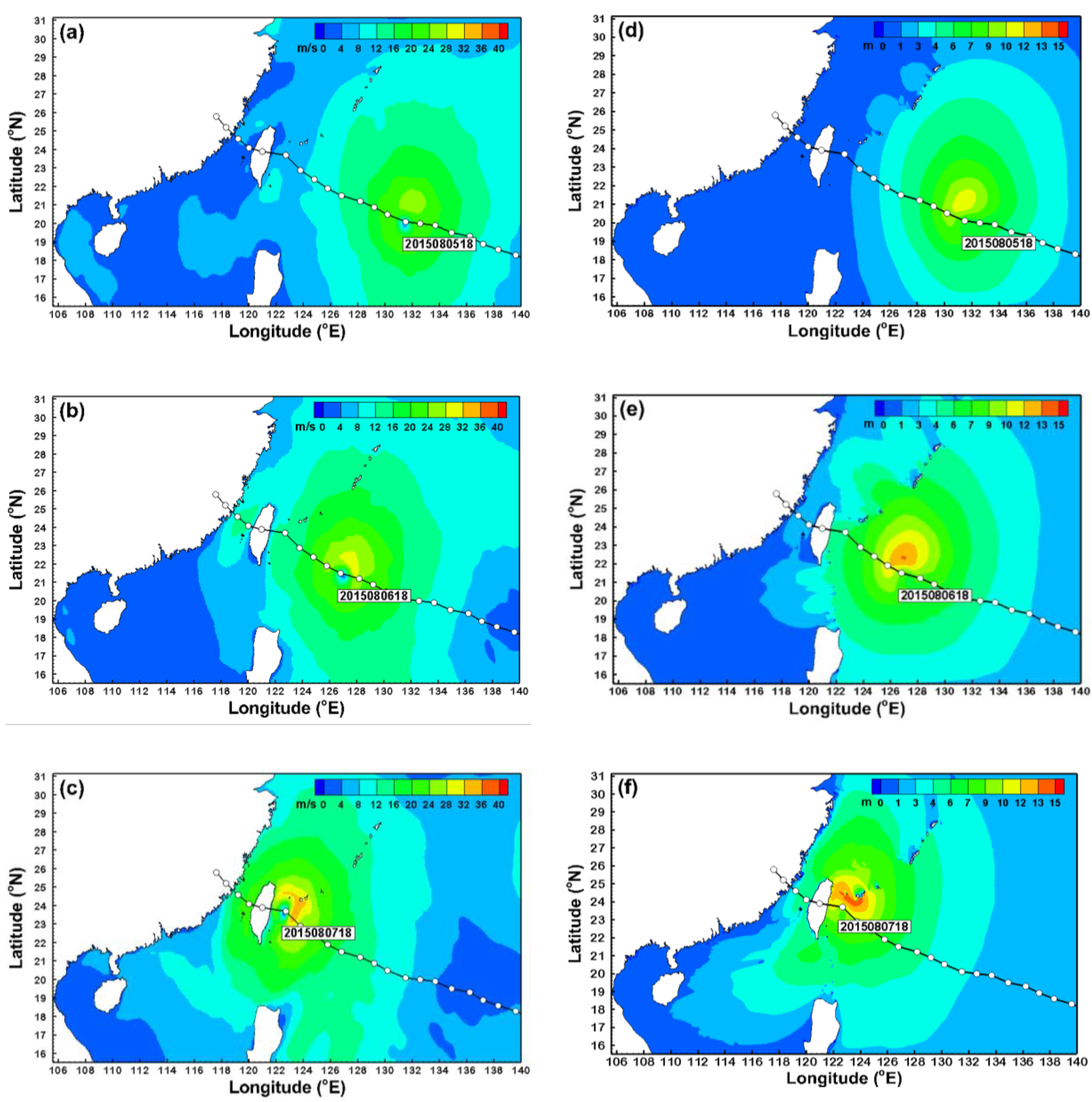
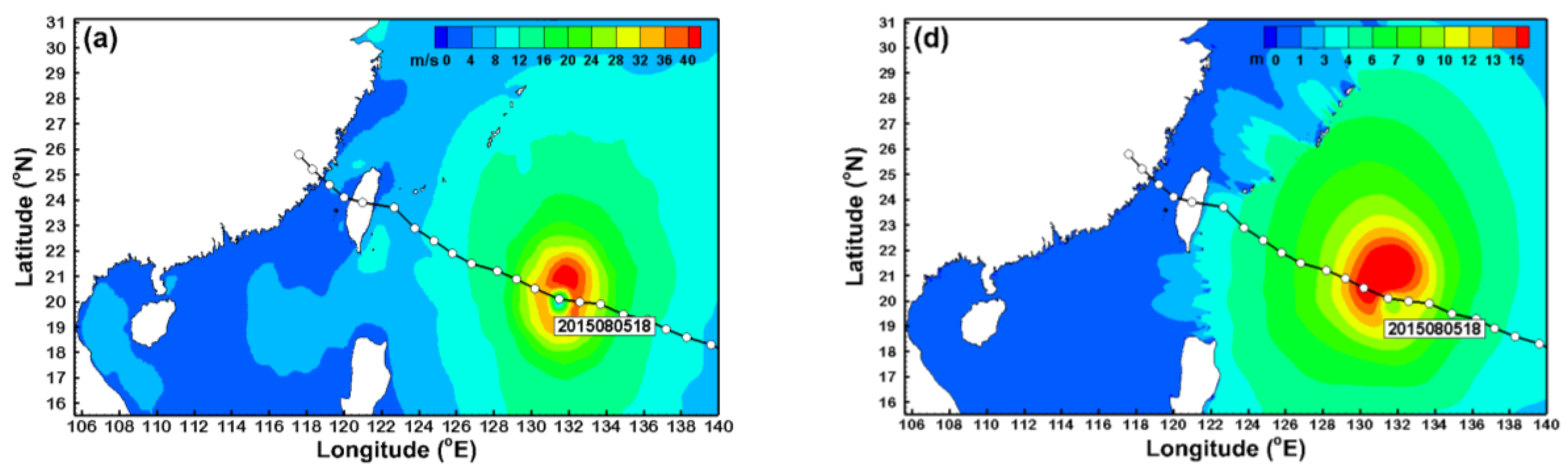
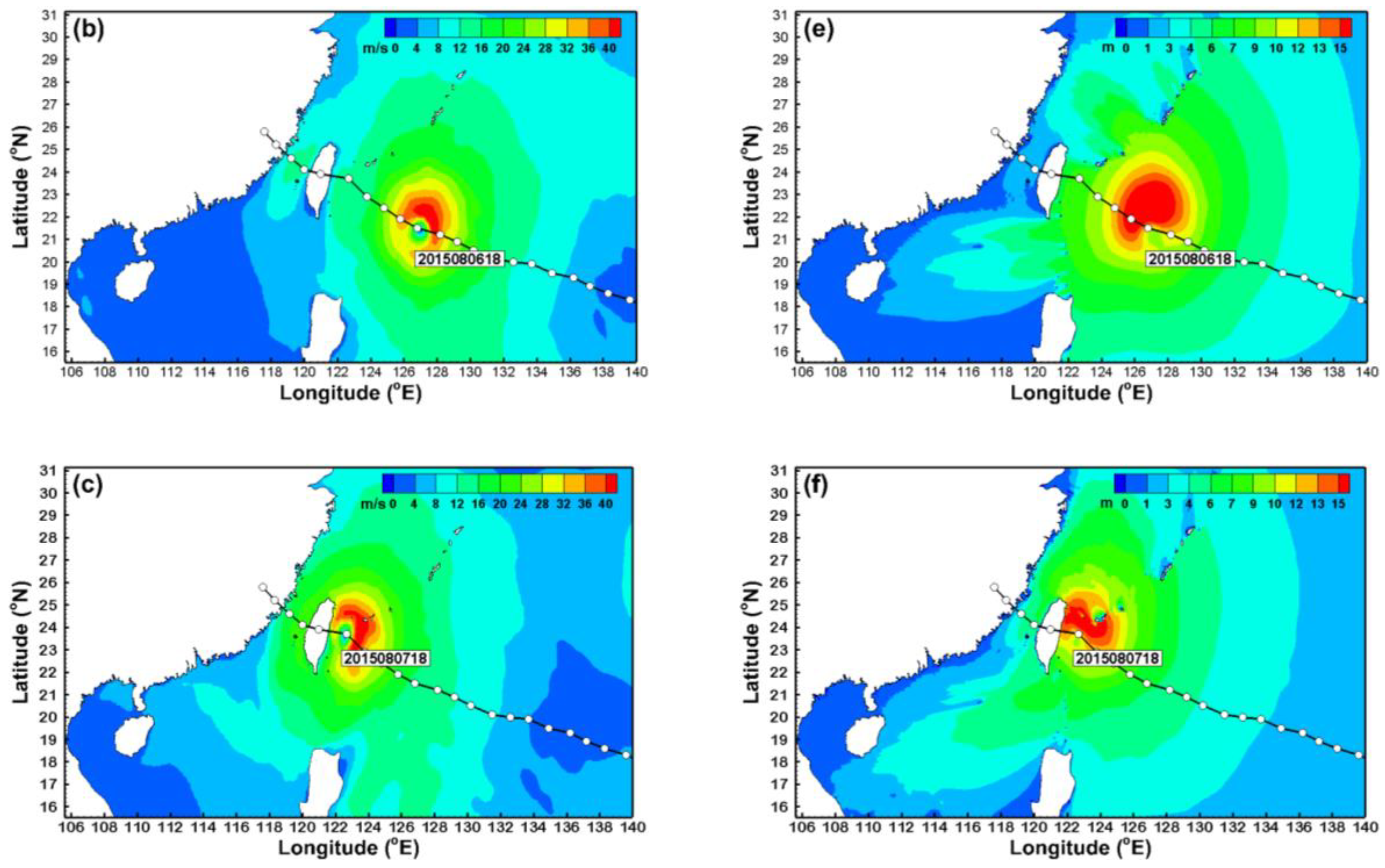
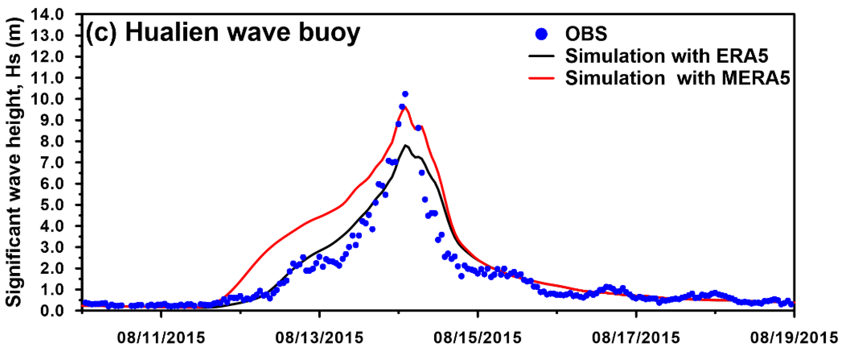
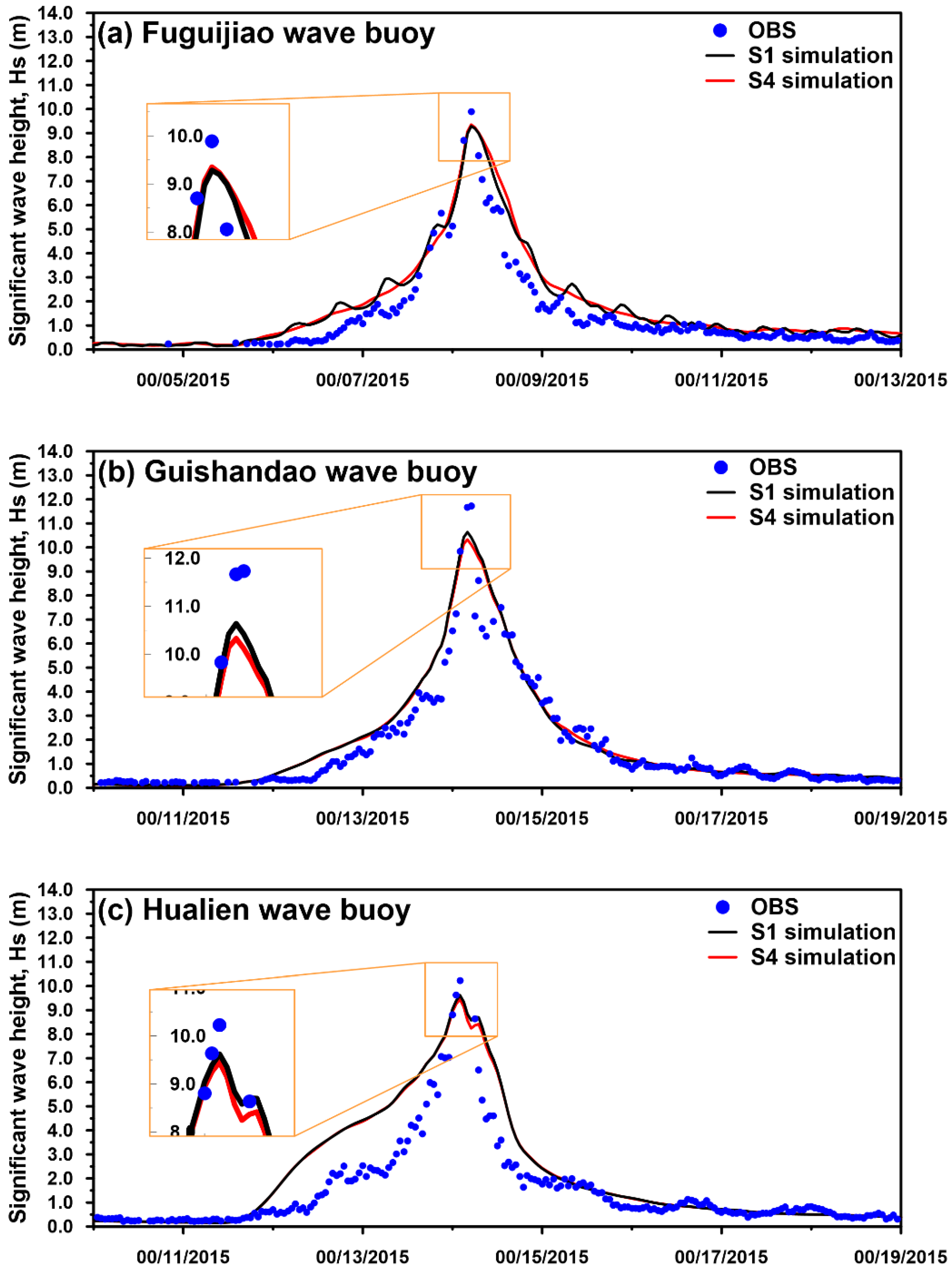
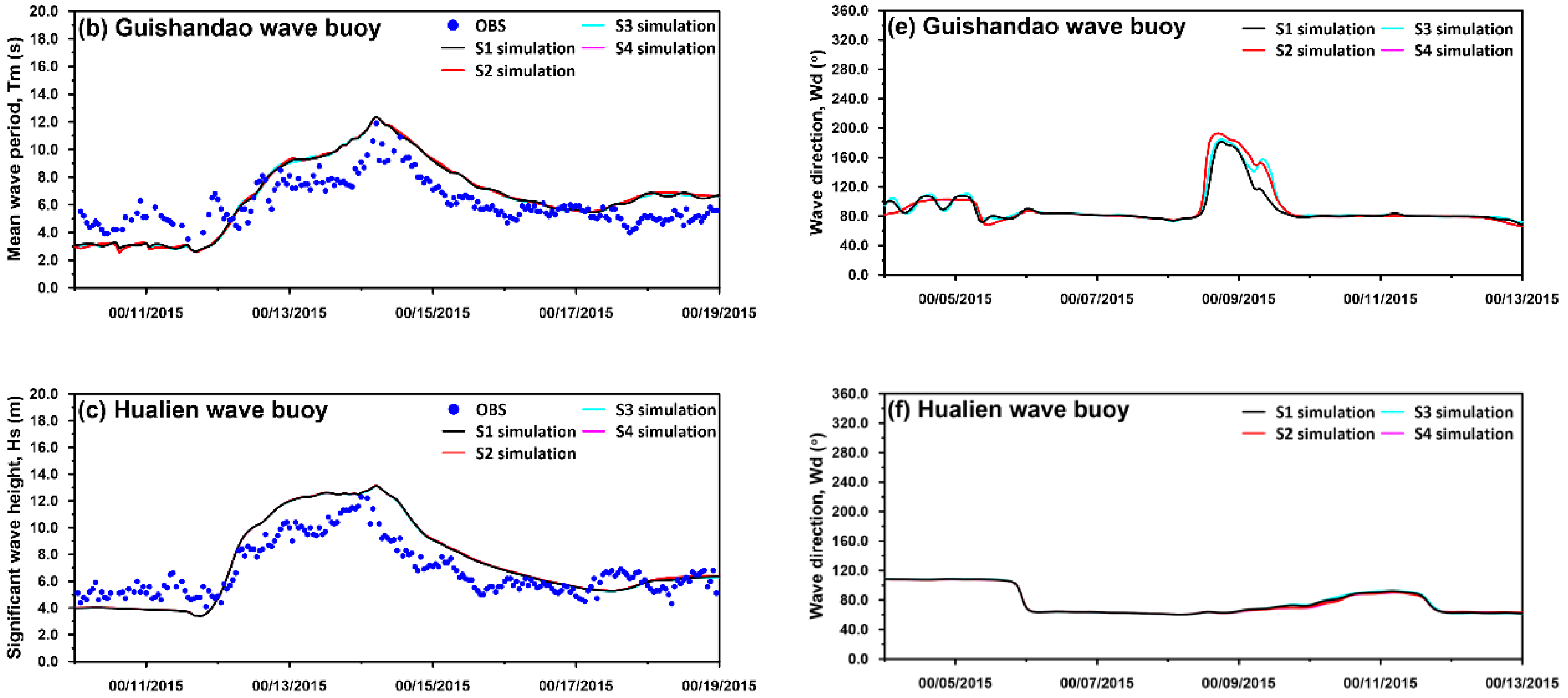
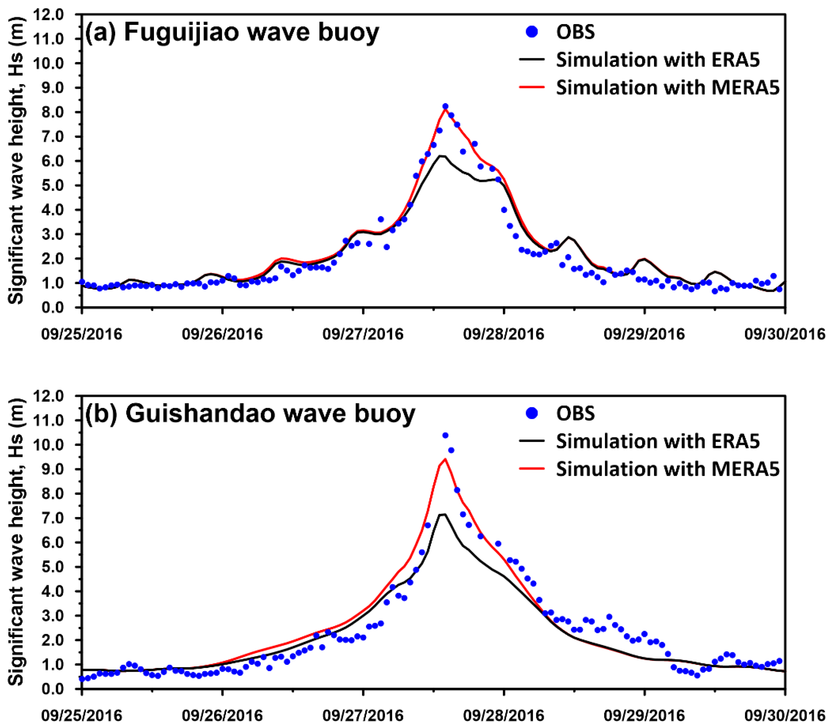
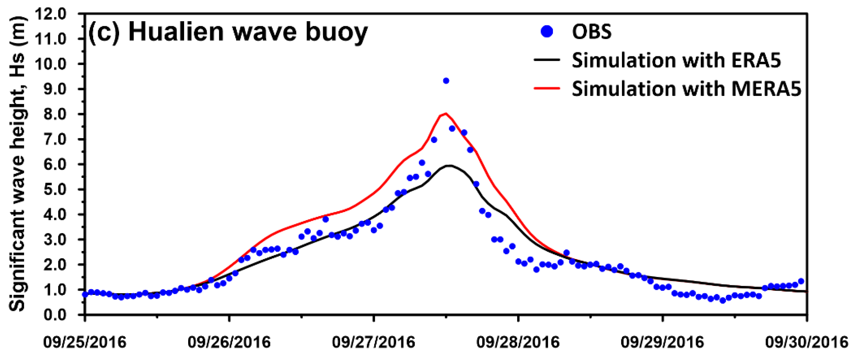
3.1. Effects of Atmospheric Forcing on Typhoon Wave Simulations

The hourly typhoon winds used in SCHISM-WWM-III were acquired from ERA5 at a horizontal resolution of 31 km and were then interpolated from the structured grid to the unstructured grid by means of the inverse distance weighting method. Figure 4a–c illustrate the instantaneous spatial distributions of the wind field during Typhoon Soudelor in 2015. As seen in Figure 4a–c, the wind speeds from the hourly ERA5 product reach only 24–36 m/s in the near-field region of Typhoon Soudelor. The instantaneous distributions of the simulated significant wave height corresponding to the hourly ERA5 winds at the specified times are displayed in Figure 4d–f. The simulated peak significant wave heights are 10–12 m in the deep-water area far from Taiwan (Figure 4d) and gradually increase to 12–13 m (Figure 4e) and 13–15 m (Figure 4f) with the typhoon’s approach to Taiwan. Figure 5a–c present snapshots of the spatial distributions of the typhoon wind field obtained from MERA5 at the same specified times as in Figure 4a–c. Increases in wind speed are obvious near the inner region of the typhoon, and the maximal wind speed reaches 36–40 m/s or even exceeds 40 m/s after modification. Figure 5d–f show that the increases in the significant wave height caused by the use of the MERA5 winds relative to the values induced by the winds from ERA5 are 1–2 m. Additionally, the areas with large significant wave heights (greater than or equal to 15 m) are extended.

Comparisons of the significant wave height time series between model simulations using the different wind forcings and the corresponding measurements are presented in Figure 6a–c for the Fuguijiao (Figure 6a), Guishandao (Figure 6b), and Hualien (Figure 6c) buoys. The peak wave heights are underestimated by 2–2.5 m for all three wave buoys when the ERA5 winds are used in SCHISM-WWM-III. The underestimations between the simulated and measured peak wave heights are reduced to 0.5–1.0 m when the winds from MERA5 are imposed in SCHISM-WWM-III. Significant improvements in the simulated typhoon wave heights are achieved when employing the MERA5 winds; therefore, the SCHISM-WWM-III model combined with the winds from MERA5 was further utilized to investigate the sensitivity of storm wave simulations to the tidal elevation and tidal current for Typhoon Soudelor in 2015.

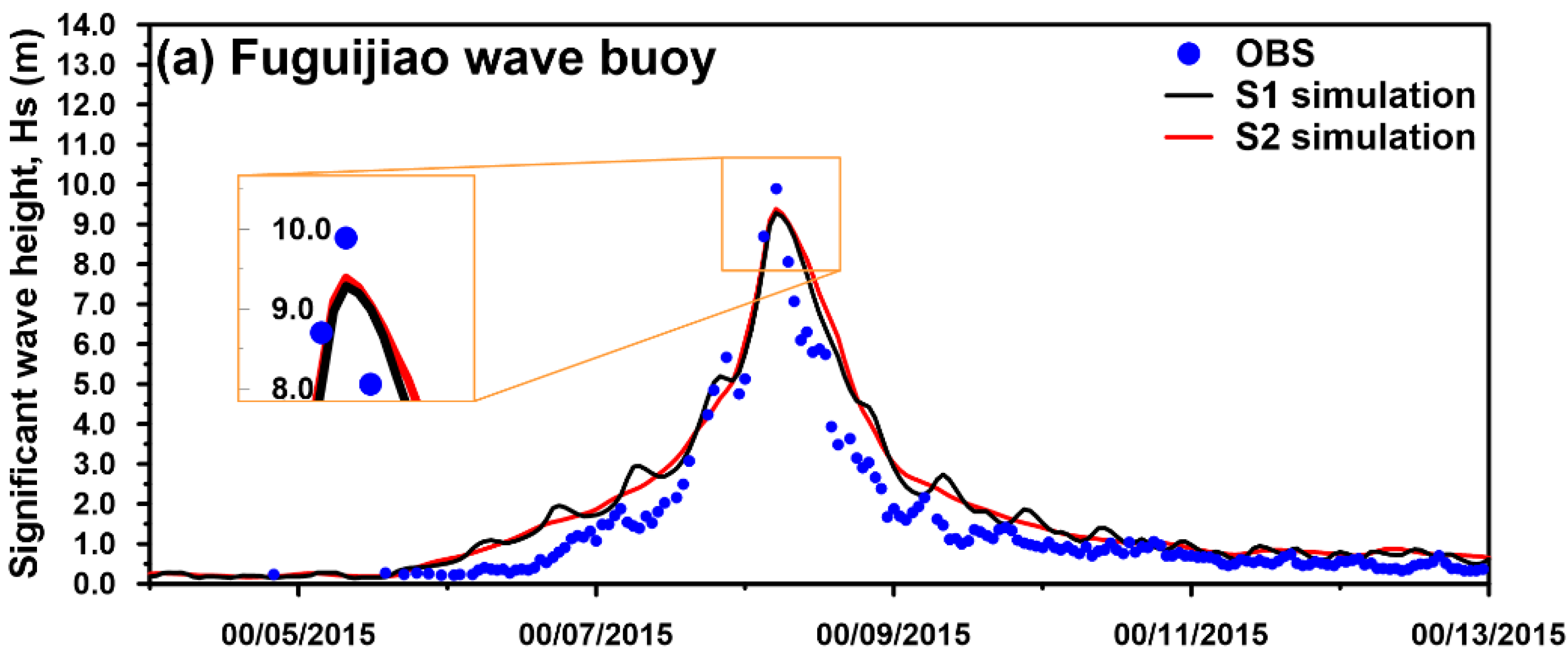
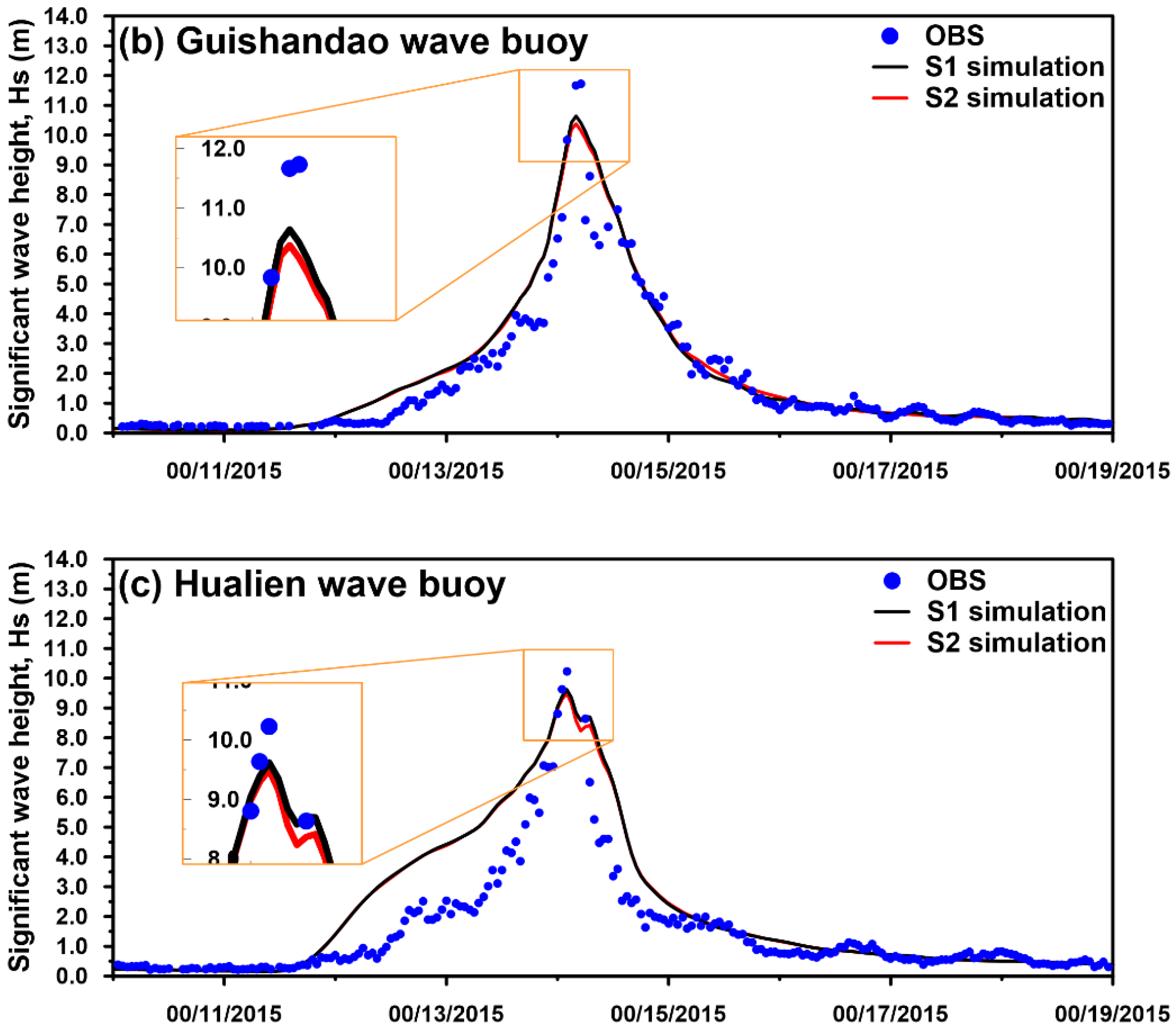
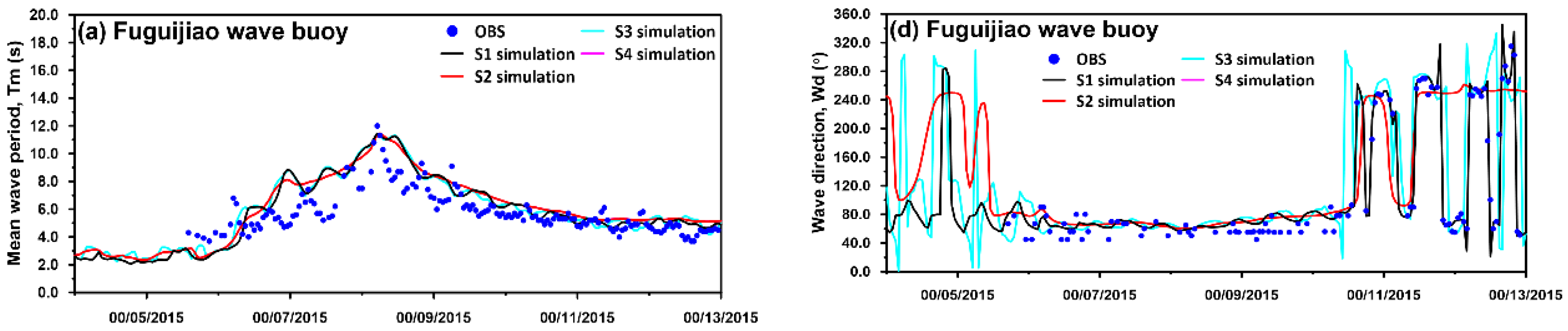
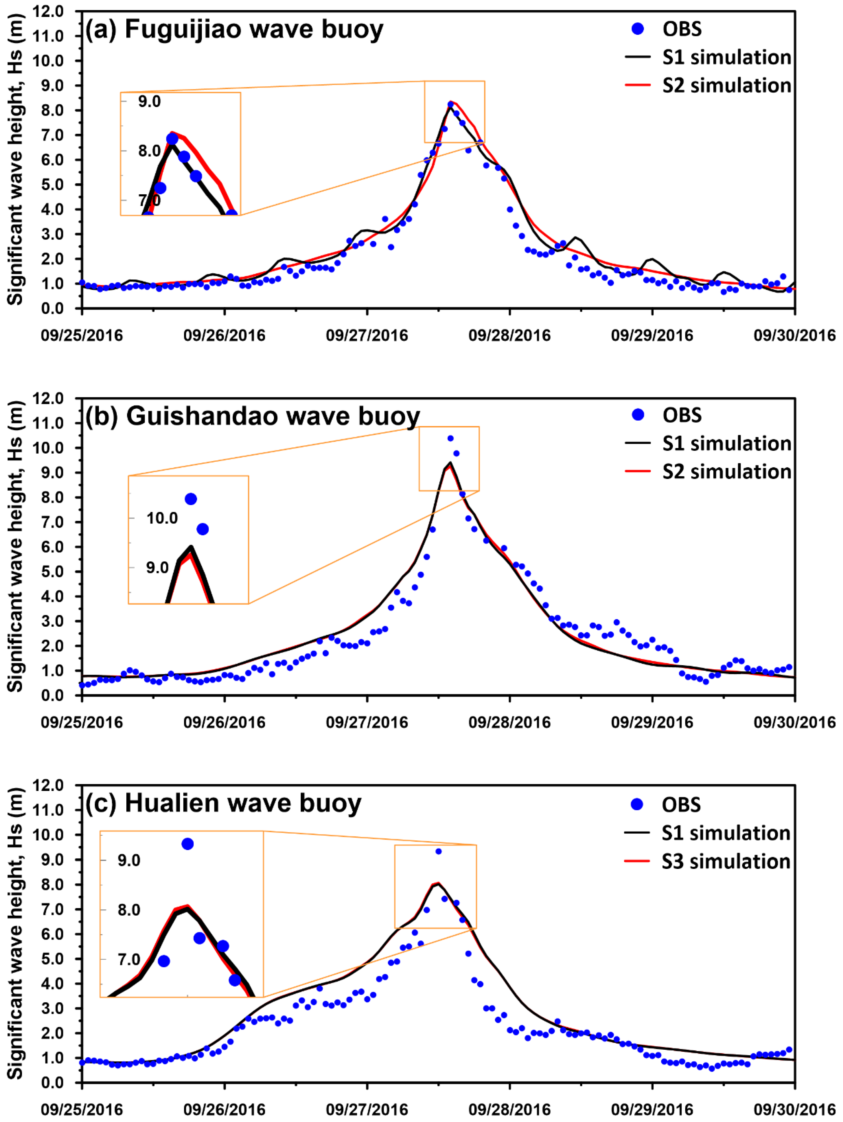
3.2. Typhoon Wave Simulation in the Absence of Tidal Current

The significant wave heights from 1–15 August in 2015 were reproduced using the MERA5-driven SCHISM-WWM-III model. Two scenarios were considered to better understand the effect of the tidal current on the wave modeling performance. One scenario was a wave simulation that included both the tidal elevation and tidal current (hereafter denoted by S1, as shown in Table 2), and the other was a wave simulation that included only the tidal elevation (hereafter denoted by S2, as shown in Table 2). Figure 7 shows comparisons of the significant wave height time series between the modeled and measured values for the Fuguijiao (Figure 7a), Guishandao (Figure 7b), and Hualien (Figure 7c) wave buoys using the winds from MERA5 in these two different scenarios. The S1 simulations show fluctuations in the significant wave height time series during the approach and retreat of the typhoon; by contrast, the S2 simulations, i.e., without the tidal current, are smoother. Notably, however, this phenomenon is only obvious at the Fuguijiao wave buoy (Figure 7a) and thus might be due to the presence of a stronger tidal current in the northern nearshore waters of Taiwan. The simulated peak significant wave heights from the S1 and S2 simulations are also depicted in a magnified form in Figure 7a–c. The peak significant wave height simulated in scenario S2 is slightly higher than that in S1 for the Fuguijiao wave buoy but is slightly lower for the Guishandao and Hualien wave buoys. Overall, the effect of the tidal current on the storm wave simulations during the period of Typhoon Soudelor in 2015 is most evident in the northern waters of Taiwan. The data issued from the industrial technology research institute of Taiwan implies that the averaged tidal current speed could be reached 0.8–1.0 m/s near the Fuguijiao wave buoy where the coastline has a cape shape, but only 0.2–0.3 m/s and 0.6–0.8 m/s in the nearshore waters adjacent to the Guishandao and Hualien wave buoys. For this reason, the typhoon wave simulations are more sensitivity to tidal current for the Fuguijiao buoy than for the others.

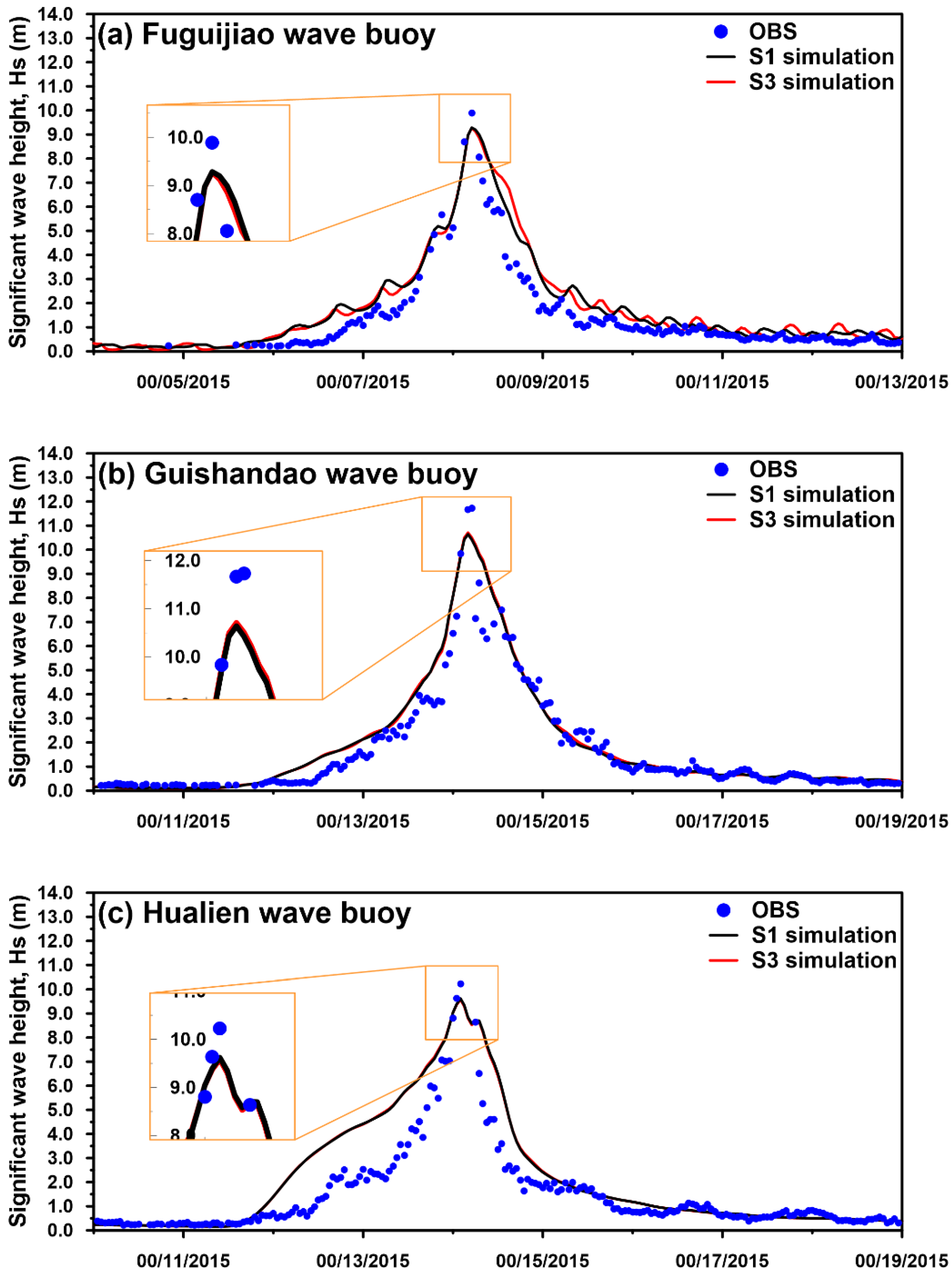
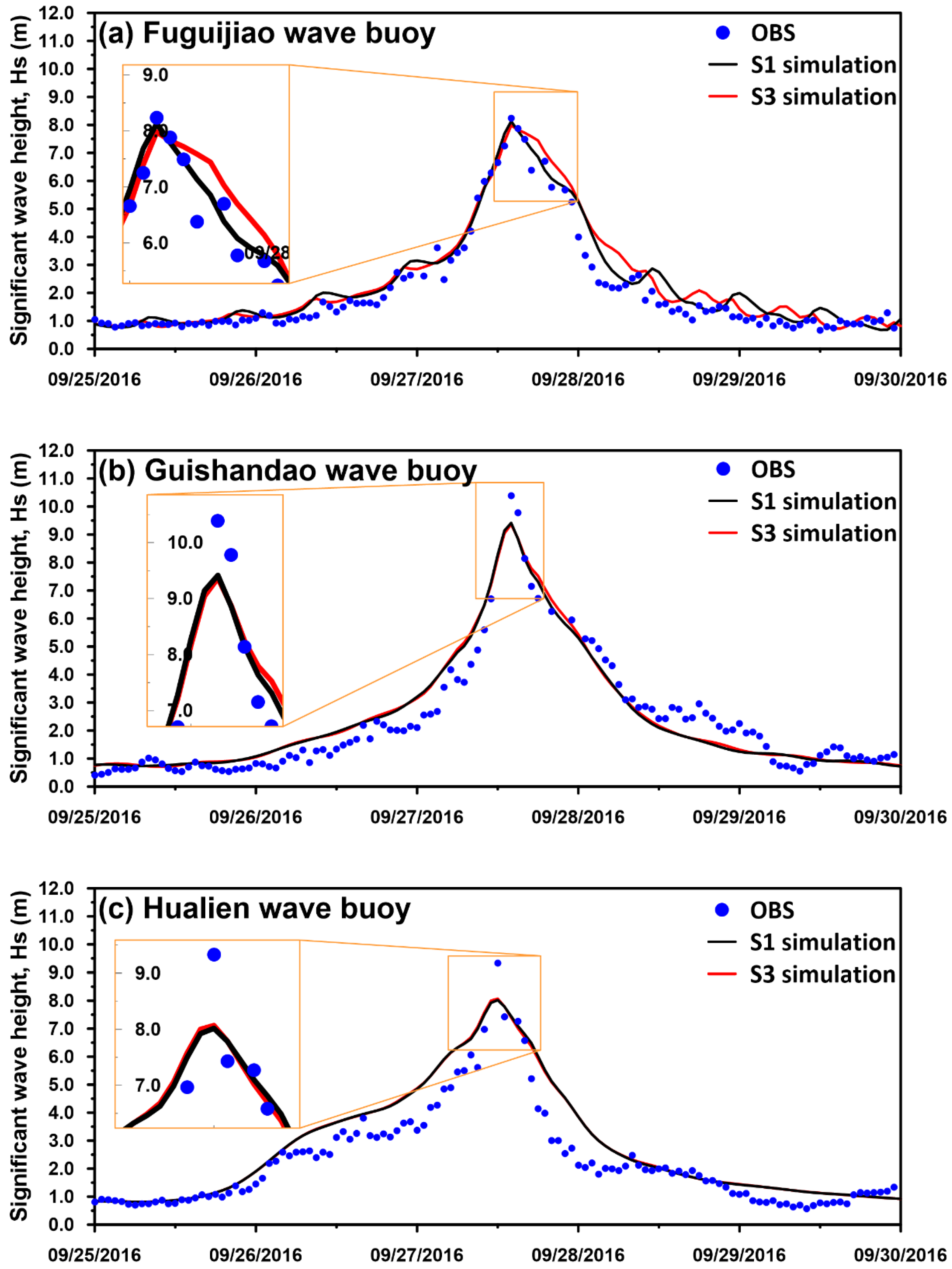
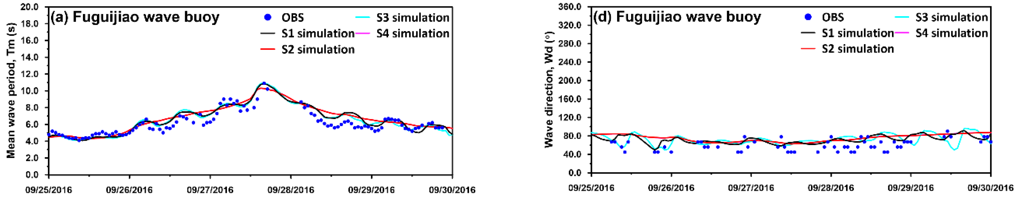
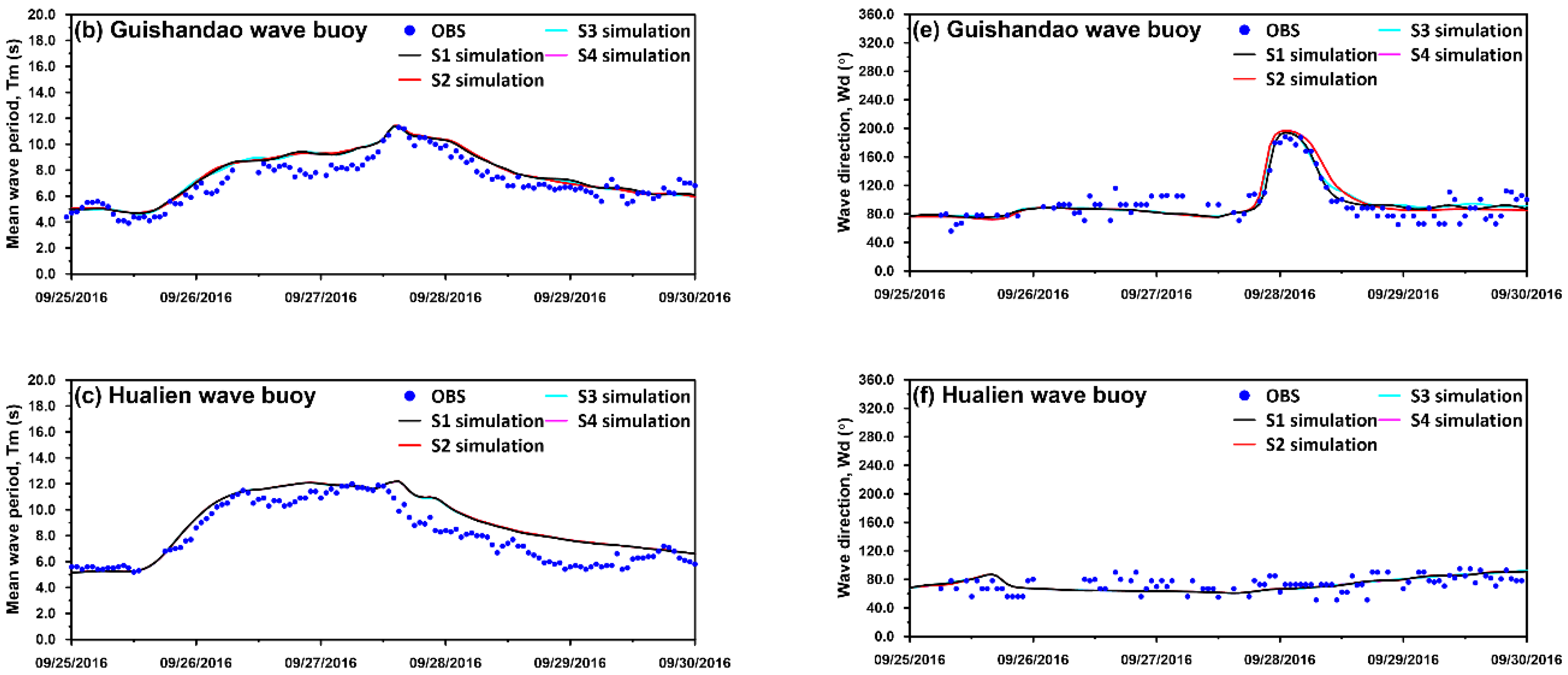
3.3. Typhoon Wave Simulation in the Absence of Tidal Elevation

As shown in Table 2, the storm wave simulation scenario that includes the tidal current but not the tidal elevation is called S3. Comparisons of the significant wave heights between the S1 and S3 simulations and the corresponding measurements for the different wave buoys are illustrated in Figure 8, where Figure 8a–c present the results for the Fuguijiao, Guishandao, and Hualien wave buoys, respectively. Fluctuations are evident in Figure 8a (for the Fuguijiao wave buoy) for the scenario in which the tidal current is included for typhoon wave modeling. Interestingly, the fluctuation amplitudes are smaller than those in the S1 simulations. Additionally, phase shifts between the S1 and S3 simulations can also be seen for the Fuguijiao wave buoy (Figure 8a). For the Guishandao (Figure 8b) and Hualien (Figure 8c) wave buoys, the S1 and S3 simulations are almost identical with regard to the time series of the simulated significant wave heights. The differences in the simulated peak wave heights between the S1 and S3 simulations are also small, as seen from the enlarged views in Figure 8a–c. The observed phenomena may be attributable to the different tidal ranges in the northern, northeastern, and eastern coastal waters of Taiwan. According to the statistics of the long-term tidal monitoring data from the CWB, the average tidal ranges are 1.61, 0.88, and 1.0 m in the northern, northeastern, and eastern coastal waters of Taiwan, respectively. Thus, the tidal range near the Fuguijiao wave buoy (in the northern waters) is approximately twice as large as those near the Guishandao (northeastern) and Hualien (eastern) wave buoys; therefore, the effect of the tidal elevation on the wave simulations is more significant for the Fuguijiao wave buoy than for the Guishandao and Hualien wave buoys.

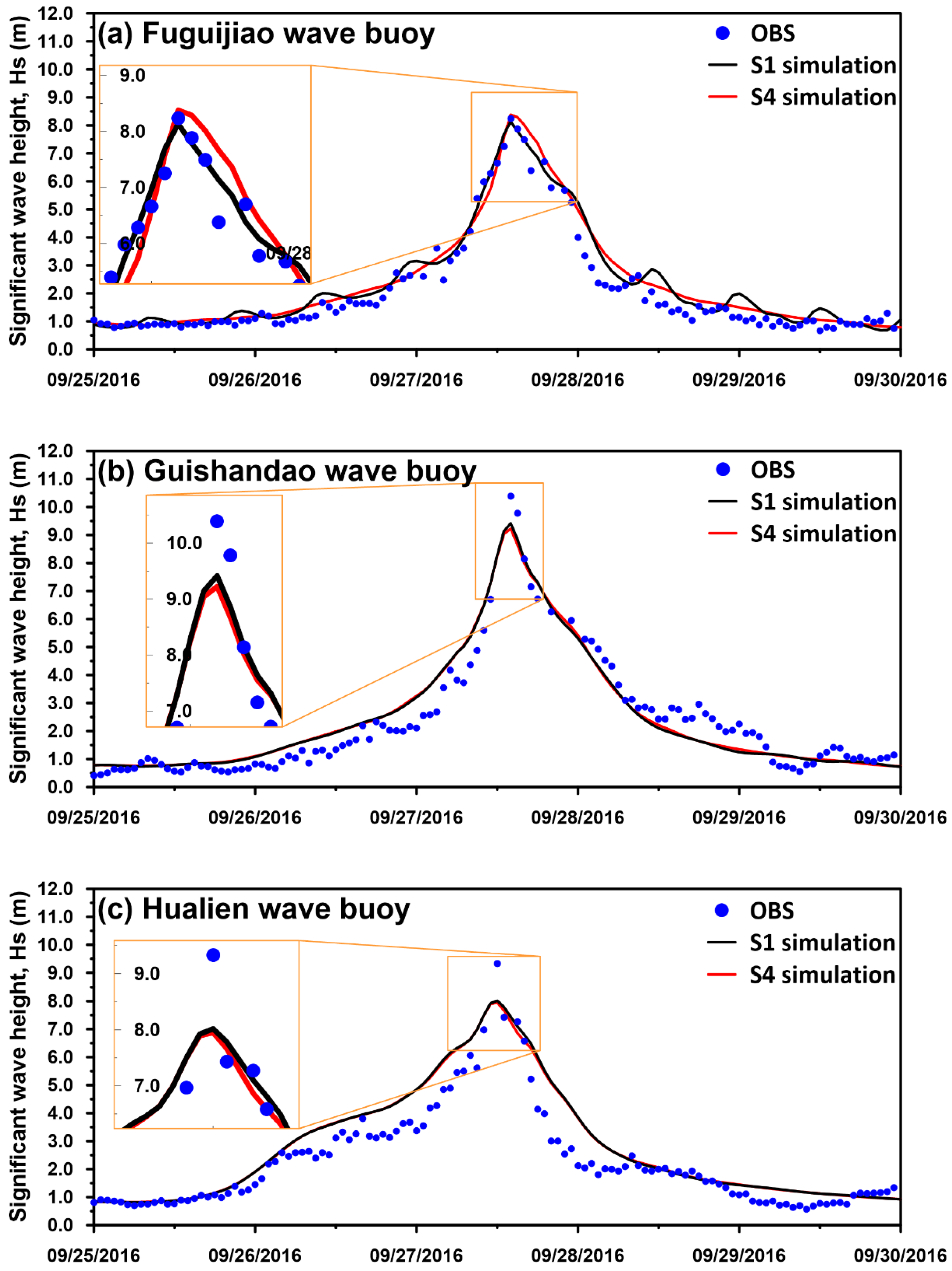
3.4. Typhoon Wave Simulation in the Absence of Both Tidal Elevation and Tidal Current

The S4 simulations can be regarded as stand-alone wave modeling because both tidal current and tidal elevation are neglected in the model (as shown in Table 2). Figure 9a–c present the model-data comparisons between the S1 and S3 simulations and the corresponding observations of the significant wave heights at the Fuguijiao (Figure 9a), Guishandao (Figure 9b), and Hualien (Figure 9c) wave buoys. As seen from Figure 9a, the significant wave height time series again becomes smooth when the tidal current is excluded from the typhoon wave simulation. Compared to the results in Figure 7a–c, no differences in the simulated significant wave height can be easily detected between the S2 (without the tidal current effect) and S4 simulations, even at the peak wave heights, for the three wave buoys. These findings reveal that the storm wave simulations are more sensitive to the absence of the tidal current than to the absence of the tidal elevation.

4. Discussion

The four model experiments conducted in the present study indicate that the simulations of the significant wave heights during Typhoon Soudelor are more sensitive to the tidal current than to the tidal elevation. To understand the effects of the tidal current and tidal elevation on other wave parameters, the sensitivity of the mean wave period and wave direction to the tidal current and tidal elevation was also investigated for the Fuguijiao, Guishandao, and Hualien wave buoys during the period of Typhoon Soudelor in 2015. The simulated results for the mean wave periods and wave directions for the different wave buoys are compared in Figure 10. The greatest inconsistencies among the S1–S4 simulations for the mean wave period (Figure 10a–c) and wave direction (Figure 10d–f, where wave direction measurements for the Guishandao and Hualien wave buoys are unavailable) are observed for the Fuguijiao wave buoy (Figure 10a,b), and the simulations in scenarios S2 and S4 are almost identical. These findings are similar to those for the simulations of the significant wave height. The results of the present study are different from those of Huang et al. [9] because the seabed slope off the eastern coast of Taiwan is very steep.

A typhoon with a very similar track and intensity that struck Taiwan in 2016, namely, Typhoon Megi (as shown in Figure 1b), was adopted to confirm the reliability of the results derived in Section 3. Figure 11a–c compare the significant wave height time series between simulations using wind data from ERA5 and MERA5 and the corresponding measurements during the period of Typhoon Megi in 2016. Although the simulated peak significant wave heights are still underestimated for the Guishandao and Hualien wave buoys (Figure 11b,c), the MERA5-driven peak significant wave heights are increased by 2 m compared to those induced by the ERA5 winds. This observation indicates that the peak storm waves can be accurately simulated under the condition that the reanalysis typhoon winds are suitably modified. Numerical experiments analogous to those conducted in Section 3 for Typhoon Soudelor in 2015 were performed to investigate the sensitivity of the wave simulations to the tidal current and tidal elevation during the period of Typhoon Megi in 2016. The results for the simulated significant wave heights in scenarios S1–S4 are compared in Figure 12, Figure 13 and Figure 14. Wave-like fluctuations are again observed in the significant wave height time series from the S1 and S2 simulations (i.e., wave modeling with and without the tidal current) for the Fuguijiao wave buoy (see the black lines in Figure 12a, Figure 13a, and Figure 14a and the red line in Figure 13a). However, this phenomenon is absent when the tidal current is excluded in the storm wave modeling (i.e., the S2 and S4 simulations; see the red lines in Figure 12a and Figure 14a). Figure 15 presents the effects of the tidal current and tidal elevation on the simulated mean wave periods and wave directions for the different wave buoys during Typhoon Megi. The simulations for the Fuguijiao wave buoy show higher sensitivity to the tidal current (as shown in Figure 15a,d) than those for the Guishandao and Hualien wave buoys do (Figure 15b–f). Thus, it is again evident that the inclusion of the tidal current is more important for typhoon wave simulation for the Fuguijiao buoy than for the others.

Although the employment of the MERA5 typhoon winds improved the peak significant wave height simulations, a rise in the wave heights outside the peak was also evident, especially for the wave buoy at Hualien (as shown in Figure 6c and Figure 11c). The adoption of the typhoon winds from the ERA5 gave better predictions of the significant wave height in the period before the peak. This phenomenon might be due to the overestimation of wind speed in the left side of typhoons by using the direct modification method. Thus, the wind speed comparisons between the ERA5, MERA5, and observation need further analysis in the future.

Saprykina et al. [46] indicated that the local wave field could be changed sharply, and the phenomenon is obvious in the presence of the adverse current. The discrepancy between the modeled and measured wave parameters in the present study could be due to the evolution of nonlinear modulation instability of waves and the increase in wave steepness on a gradually increasing adverse current.

5. Summary and Conclusions

This paper investigated the role of the tidal current and tidal elevation in wave simulations for the nearshore waters of Taiwan during typhoon events. A large computational domain with a high-resolution, unstructured-grid mesh was developed, and a fully coupled circulation-wave model, SCHISM-WWM-III, was applied to simulate the typhoon waves. The hourly typhoon winds from ERA5 and a modification of the original ERA5 product (MERA5) were considered as the atmospheric conditions for SCHISM-WWM-III to determine the optimal wind source for storm wave modeling. The performance achieved when adopting the MERA5 typhoon winds for significant wave height simulation was better than that achieved using the ERA5 winds. The simulated peak significant wave heights could be increased by 1.0–2.0 m through the utilization of the MERA5 winds for Typhoon Soudelor in 2015 and Typhoon Megi in 2016. A series of model experiments was then designed and conducted using SCHISM-WWM-III combined with the MERA5 wind data. The results of the analysis reveal that the tidal current is influential in the simulation of storm waves in the northern nearshore waters of Taiwan, where a stronger tidal current is present. The tidal current affects the simulation of not only the significant wave height but also the mean wave period and wave direction in the same nearshore area for both Typhoon Soudelor in 2015 and Typhoon Megi in 2016. Regarding the effect of the tidal elevation on the simulation of typhoon waves, the sea area in the northern waters of Taiwan is slightly sensitive to whether the tidal elevation is included in the model because the tidal range is larger in this area than in the northeastern and eastern waters. In summary, the inclusion of both the tidal current and tidal elevation is necessary for accurate sea state modeling in typhoon wave simulations, and this is particularly true for nearshore waters with a strong tidal current and a large tidal range. Another important finding is that, even with the imposition of fifth-generation reanalysis typhoon winds on the circulation-wave model, the significant wave heights induced by typhoons are still underestimated. The direct modification method applied in the present study is an alternative approach for improving the simulation of the peak wave heights while maintaining a reliable structure of the entire typhoon wind field. In future research on the sensitivity of storm wave modeling, it will be important to investigate a wider variety of typhoons with different tracks.

References

1. Shao, Z.; Liang, B.; Li, H.; Wu, G.; Wu, Z. Blended wind fields for wave modeling of tropical cyclones in the South China Sea and East China Sea. Appl. Ocean Res. 2018, 71, 20–33. [Google Scholar] [CrossRef]
2. Shih, H.-J.; Chang, C.-H.; Chen, W.-B.; Lin, L.-Y. Identifying the Optimal Offshore Areas for Wave Energy Converter Deployments in Taiwanese Waters Based on 12-Year Model Hindcasts. Energies 2018, 11, 499. [Google Scholar] [CrossRef] [Green Version]
3. Chang, C.-H.; Shih, H.-J.; Chen, W.-B.; Su, W.-R.; Lin, L.-Y.; Yu, Y.-C.; Jang, J.-H. Hazard Assessment of Typhoon-Driven Storm Waves in the Nearshore Waters of Taiwan. Water 2018, 10, 926. [Google Scholar] [CrossRef] [Green Version]
4. Lewis, M.; Bates, P.; Horsburgh, K.; Neal, J.; Schumann, G. A storm surge inundation model of the northern Bay of Bengal using publicly available data. Q. J. R. Meteorol. Soc. 2013, 139, 358–369. [Google Scholar] [CrossRef]
5. Wang, T.; Yang, Z.; Wu, W.-C.; Grear, M. A Sensitivity Analysis of the Wind Forcing Effect on the Accuracy of Large-Wave Hindcasting. J. Mar. Sci. Eng. 2018, 3, 139. [Google Scholar] [CrossRef] [Green Version]
6. Longuet-Higgins, M.S.; Stewart, R.W. Radiation stress in water waves: A physical discussion with applications. Deep Sea Res. 1964, 11, 529–562. [Google Scholar]
7. Phillips, O.M. The Dynamics of Upper Ocean; Cambridge University Press: New York, NY, USA, 1977; 336p. [Google Scholar]
8. Large, W.G.; Pond, S. Open ocean momentum fluxes in moderate to strong winds. J. Phys. Oceanogr. 1981, 11, 324–336. [Google Scholar] [CrossRef] [Green Version]
9. Huang, Y.; Weisberg, R.H.; Zheng, L. Coupling of surge and waves for an Ivan-like hurricane impacting the Tampa Bay, Florida region. J. Geophys. Res. 2010, 115, C12009. [Google Scholar] [CrossRef]
10. Hsiao, S.-C.; Chen, H.; Chen, W.-B.; Chang, C.-H.; Lin, L.-Y. Quantifying the contribution of nonlinear interactions to storm tide simulations during a super typhoon event. Ocean Eng. 2019, 194, 106661. [Google Scholar] [CrossRef]
11. Rusu, L.; Bernardino, M.; Guedes Soares, C. Influence of Wind Resolution on Prediction of Waves Generated in an Estuary. J. Coast. Res. 2009, 56, 1419–1423. [Google Scholar]
12. Van Vledder, G.P.; Akpınar, A. Wave model predictions in the Black Sea: Sensitivity to wind fields. Appl. Ocean Res. 2015, 53, 161–178. [Google Scholar] [CrossRef]
13. Zhang, Y.J.; Ye, F.; Stanev, E.V.; Grashorn, S. Seamless cross-scale modelling with SCHISM. Ocean Modell. 2016, 102, 64–81. [Google Scholar] [CrossRef] [Green Version]
14. Zhang, Y.J.; Baptista, A.M. SELFE: A semi-implicit Eulerian-Lagrangian finite-element model for cross-scale ocean circulation. Ocean Modell. 2008, 21, 71–96. [Google Scholar] [CrossRef]
15. Wang, H.V.; Loftis, J.D.; Liu, Z.; Forrest, D.; Zhang, J. The storm surge and sub-grid inundation modeling in New York City during hurricane Sandy. J. Mar. Sci. Eng. 2014, 2, 226–246. [Google Scholar] [CrossRef] [Green Version]
16. Chen, W.-B.; Liu, W.-C. Modeling flood inundation Induced by river flow and storm surges over a river basin. Water 2014, 6, 3182–3199. [Google Scholar] [CrossRef] [Green Version]
17. Chen, W.-B.; Liu, W.-C. Assessment of storm surge inundation and potential hazard maps for the southern coast of Taiwan. Nat. Hazards 2016, 82, 591–616. [Google Scholar] [CrossRef]
18. Chen, Y.-M.; Liu, C.-H.; Shih, H.-J.; Chang, C.-H.; Chen, W.-B.; Yu, Y.-C.; Su, W.-R.; Lin, L.-Y. An Operational Forecasting System for Flash Floods in Mountainous Areas in Taiwan. Water 2019, 11, 2100. [Google Scholar] [CrossRef] [Green Version]
19. Chen, W.-B.; Chen, H.; Lin, L.-Y.; Yu, Y.-C. Tidal Current Power Resource and Influence of Sea-Level Rise in the Coastal Waters of Kinmen Island, Taiwan. Energies 2017, 10, 652. [Google Scholar] [CrossRef] [Green Version]
20. Chen, W.-B.; Liu, W.-C. Investigating the fate and transport of fecal coliform contamination in a tidal estuarine system using a three-dimensional model. Mar. Pollut. Bull. 2017, 116, 365–384. [Google Scholar] [CrossRef]
21. Powell, M.D.; Vickery, P.J.; Reinhold, T.A. Reduced drag coefficient for high wind speeds in tropical cyclones. Nature 2003, 422, 279–283. [Google Scholar] [CrossRef]
22. Smith, S.D. Wind stress and heat flux over the ocean in gale force winds. J. Phys. Oceanogr. 1980, 10, 709–726. [Google Scholar] [CrossRef]
23. Longuet-Higgins, M.S.; Stewart, R.W. Radiation stress and transport in gravity wave, with application to ‘surf beat’. J. Fluid Mech. 1962, 13, 485–504. [Google Scholar] [CrossRef]
24. Komen, G.J.; Cavaleri, L.; Donelan, M.; Hasselmann, K.; Hasselmann, S.; Janssen, P.A.E.M. Dynamics and Modelling of Ocean Waves; Cambridge University Press: Cambridge, UK, 1994; p. 532. [Google Scholar]
25. Roland, A. Development of WWM II: Spectral Wave Modeling on Unstructured Meshes. Ph.D. Thesis, Institute of Hydraulic and Water Resources Engineering, Technische Universität Darmstadt, Darmstadt, Germany, 2009. [Google Scholar]
26. Hsu, T.-W.; Ou, S.-H.; Liau, J.-M. Hindcasting nearshore wind waves using a FEM code for SWAN. Coastal Eng. 2005, 52, 177–195. [Google Scholar] [CrossRef]
27. Booij, N.; Ris, R.C.; Holthuijsen, L.H. A third-generation wave model for coastal regions. 1. Model description and validation. J. Geophys. Res. 1999, 104, 7649–7666. [Google Scholar] [CrossRef] [Green Version]
28. Su, W.-R.; Chen, H.; Chen, W.-B.; Chang, C.-H.; Lin, L.-Y.; Jang, J.-H.; Yu, Y.-C. Numerical investigation of wave energy resources and hotspots in the surrounding waters of Taiwan. Renew. Energy 2018, 118, 814–824. [Google Scholar] [CrossRef]
29. Hasselmann, K.; Barnett, T.P.; Bouws, E.; Carlson, H.; Cartwright, D.E.; Enke, K. Measurements of Wind-Wave Growth and Swell Decay during the Joint North Sea Wave Project (JONSWAP); Deutsche Hydrographische Institut (DHI): Hamburg, Germany, 1973; Volume 12. [Google Scholar]
30. Hasselmann, S.; Hasselmann, K.; Allender, J.H.; Barnett, T.P. Computations and parameterizations of the non-linear energy transfer in a gravity-wave spectrum, Part 2: Parameterizations of the non-linear energy transfer for application in wave models. J. Phys. Oceanogr. 1985, 15, 1378–1391. [Google Scholar] [CrossRef] [Green Version]
31. Roland, A.; Zhang, Y.J.; Wang, H.V.; Meng, Y.; Teng, Y.-C.; Maderich, V.; Brovchenko, I.; Dutour-Sikiric, M.; Zanke, U. A fully coupled 3D wave-current interaction model on unstructured grids. J. Geophys. Res. 2012, 117, C00J33. [Google Scholar] [CrossRef]
32. Orton, P.; Georgas, N.; Blumberg, A.; Pullen, J. Detailed modeling of recent severe storm tides in estuaries of the New York City region. J. Geophys. Res. 2012, 117, C09030. [Google Scholar] [CrossRef] [Green Version]
33. Zheng, L.; Weisberg, R.H.; Huang, Y.; Luettich, R.A.; Westerink, J.J.; Kerr, P.C.; Donahue, A.S.; Grane, G.; Akli, L. Implications from the comparisons between two- and three-dimensional model simulations of the Hurricane Ike storm surge. J. Geophys. Res. Ocean. 2013, 118, 3350–3369. [Google Scholar] [CrossRef] [Green Version]
34. Zhang, H.; Sheng, J. Estimation of extreme sea levels over the eastern continental shelf of North America. J. Geophys. Res. Ocean. 2013, 118, 6253–6273. [Google Scholar] [CrossRef]
35. Muis, S.; Verlaan, M.; Winsemius, H.C.; Aerts, J.C.J.H.; Ward, P.J. A global reanalysis of storm surges and extreme sea levels. Nat. Commun. 2016, 7, 11969. [Google Scholar] [CrossRef] [PubMed] [Green Version]
36. Marsooli, R.; Lin, N. Numerical modeling of historical storm tides and waves and their interactions along the U.S. East and Gulf Coasts. J. Geophys. Res. Ocean. 2018, 123, 3844–3874. [Google Scholar] [CrossRef] [Green Version]
37. Chen, W.-B.; Chen, H.; Hsiao, S.-C.; Chang, C.-H.; Lin, L.-Y. Wind forcing effect on hindcasting of typhoon-driven extreme waves. Ocean Eng. 2019, 188, 106260. [Google Scholar] [CrossRef]
38. Murty, P.N.L.; Srinivas, K.S.; Rao Rama Pattabhi, E.; Bhaskaran, P.K.; Shenoi, S.S.C.; Padmanabham, J. Improved cyclone wind fields over the Bay of Bengal and their application in storm surge and wave computations. Appl. Ocean Res. 2020, 95, 102048. [Google Scholar] [CrossRef]
39. Pan, Y.; Chen, Y.P.; Li, J.X.; Ding, X.L. Improvement of wind field hindcasts for tropical cyclones. Water Sci. Eng. 2016, 9, 58–66. [Google Scholar] [CrossRef] [Green Version]
40. Li, J.; Pan, S.; Chen, Y.; Fan, Y.M.; Pan, Y. Numerical estimation of extreme waves and surges over the northwest Pacific Ocean. Ocean Eng. 2018, 153, 225–241. [Google Scholar] [CrossRef]
41. Qiao, W.; Song, J.; He, H.; Li, F. Application of different wind filed models and wave boundary layer model to typhoon waves numerical simulation in WAVEWATCH III model. Tellus A 2019, 7, 1657552. [Google Scholar] [CrossRef] [Green Version]
42. Hsiao, S.-C.; Chen, H.; Wu, H.-L.; Chen, W.-B.; Chang, C.-H.; Guo, W.-D.; Chen, Y.-M.; Lin, L.-Y. Numerical Simulation of Large Wave Heights from Super Typhoon Nepartak (2016) in the Eastern Waters of Taiwan. J. Mar. Sci. Eng. 2020, 8, 217. [Google Scholar] [CrossRef] [Green Version]
43. Knaff, J.A.; Sampson, C.R.; Demaria, M.; Marchok, T.P.; Gross, J.M.; Mcadie, C.J. Statistical Tropical Cyclone Wind Radii Prediction Using Climatology and Persistence. Weather Forecast. 2007, 22, 781–791. [Google Scholar] [CrossRef]
44. Zu, T.; Gana, J.; Erofeevac, S.Y. Numerical study of the tide and tidal dynamics in the South China Sea. Deep Sea Res. Part I 2008, 55, 137–154. [Google Scholar] [CrossRef]
45. Liu, Z.; Wang, H.; Zhang, Y.J.; Magnusson, L.; Loftis, J.D. Cross-scale modeling of storm surge, tide and inundation in Mid-Atlantic Bight and New York City during Hurricane Sandy 2012. Estuar. Coast. Shelf Sci. 2020, 233, 106544. [Google Scholar] [CrossRef]
46. Saprykina, Y.V.; Kuznetsov, S.Y.; Shugan, I.V.; Hwung, H.H.; Hsu, W.Y.; Yang, R.Y. Discrete evolution of the surface wave spectrum on a nonuniform adverse current. Dokl. Earth Sci. 2015, 464, 1075–1079. [Google Scholar] [CrossRef]
Figure 1. Tracks, central positions, and arrival times of (a) Typhoon Soudelor in 2015 and (b) Typhoon Megi in 2016. The points marked in cyan are the locations of the wave buoys adopted in the present study (Information of typhoons were provided by the Regional Specialized Meteorological Center (RSMC) Tokyo-Typhoon Center).
Jmse 08 00731 g001
Figure 2. Coverage of the computational domain and its unstructured triangular mesh.
Jmse 08 00731 g002
Figure 3. Distribution of seafloor elevations in the computational domain of Semi-implicit Cross-scale Hydroscience Integrated System Model Wind Wave Model version III (SCHISM-WWM-III).
Jmse 08 00731 g003
Figure 4. Instantaneous distributions of the hourly wind field from the fifth-generation global atmospheric reanalysis (ERA5) product (ac) and the corresponding simulated significant wave heights (df) for Typhoon Soudelor at the specified times in 2015.
Jmse 08 00731 g004
Figure 5. Instantaneous distributions of the hourly wind field from the modified fifth-generation global atmospheric reanalysis (MERA5) product (ac) and the corresponding simulated significant wave heights (df) for Typhoon Soudelor at the specified times in 2015.
Jmse 08 00731 g005aJmse 08 00731 g005b
Figure 6. Comparison of the time series of the significant wave heights between simulations using different wind forcings and the corresponding measurements for the (a) Fuguijiao, (b) Guishandao, and (c) Hualien wave buoys during the period of Typhoon Soudelor in 2015.
Jmse 08 00731 g006aJmse 08 00731 g006b
Figure 7. Comparison of the time series of the significant wave heights between the wave simulation that included both the tidal elevation and tidal current (S1) and the wave simulation that included only the tidal elevation (S2) and the corresponding measurements for the (a) Fuguijiao, (b) Guishandao, and (c) Hualien wave buoys during the period of Typhoon Soudelor in 2015.
Jmse 08 00731 g007aJmse 08 00731 g007b
Figure 8. Comparison of the time series of the significant wave heights between the S1 and the storm wave simulation scenario that includes the tidal current but not the tidal elevation (S3) and the corresponding measurements for the (a) Fuguijiao, (b) Guishandao, and (c) Hualien wave buoys during the period of Typhoon Soudelor in 2015.
Jmse 08 00731 g008
Figure 9. Comparison of the time series of the significant wave heights between the S1 and stand-alone wave modeling (S4) simulations and the corresponding measurements for the (a) Fuguijiao, (b) Guishandao, and (c) Hualien wave buoys during the period of Typhoon Soudelor in 2015.
Jmse 08 00731 g009
Figure 10. Comparison of the time series of the mean wave periods (ac) and wave directions (df)between the S1, S2, S3, and S4 simulations and the corresponding measurements for the Fuguijiao (a,d), Guishandao (b,e), and Hualien (c,f) wave buoys during the period of Typhoon Soudelor in 2015.
Jmse 08 00731 g010aJmse 08 00731 g010b
Figure 11. Comparison of the time series of the significant wave heights between simulations using different wind forcings and the corresponding measurements for the (a) Fuguijiao, (b) Guishandao, and (c) Hualien wave buoys during the period of Typhoon Megi in 2016.
Jmse 08 00731 g011aJmse 08 00731 g011b
Figure 12. Comparison of the time series of the significant wave heights between the S1 and S2 simulations and the corresponding measurements for the (a) Fuguijiao, (b) Guishandao, and (c) Hualien wave buoys during the period of Typhoon Megi in 2016.
Jmse 08 00731 g012
Figure 13. Comparison of the time series of the significant wave heights between the S1 and S3 simulations and the corresponding measurements for the (a) Fuguijiao, (b) Guishandao, and (c) Hualien wave buoys during the period of Typhoon Megi in 2016.
Jmse 08 00731 g013
Figure 14. Comparison of the time series of the significant wave heights between the S1 and S4 simulations and the corresponding measurements for the (a) Fuguijiao, (b) Guishandao, and (c) Hualien wave buoys during the period of Typhoon Megi in 2016.
Jmse 08 00731 g014
Figure 15. Comparison of the time series of the mean wave periods (ac) and wave directions (df) between the S1, S2, S3, and S4 simulations and the corresponding measurements for the Fuguijiao (a,d), Guishandao (b,e), and Hualien (c,f) wave buoys during the period of Typhoon Megi in 2016.
Jmse 08 00731 g015aJmse 08 00731 g015b