Application of the SOSim v2 Model to Spills of Sunken Oil in Rivers

Abstract

Sunken oil transport processes in rivers differ from those in oceans, and currently available models may not be generally applicable to sunken oil in river settings. The open-source Subsurface Oil Simulator (SOSim) model has been expanded to handle spills of sunken oil in navigable rivers, utilizing Bayesian inference to integrate field concentration data with bathymetric data to predict the location and movement of sunken oil. A novel prior likelihood function incorporates bathymetric input, with sampling grid and default parameters adapted appropriately for rivers. SOSim v2 was demonstrated versus field observations taken following the M/T (Motor Tanker) Athos I oil spill. The model was also modified to operate in 1-D, to assess the longitudinal distribution of sunken oil in a non-navigable river using available poling data collected following the Enbridge Kalamazoo River oil spill in 2010. Results of both case studies were consistent with observed data and local bathymetry in 2-D and 1-D, and the model is suggested as a complement to deterministic models for oil spill emergency response in rivers.

1. Introduction

Inland oil spills, such as in rivers and lakes, from rail, pipeline, or nearby storage facilities occur more frequently than oceanic spills, but involve lesser volumes of oil [1]. Further, spills in inland waters are expected to increase due to the rise in rail transport and pipeline routes across rivers [2,3,4]. Trains may derail and pipelines may burst, causing oil to enter the inland waterbody directly, or in runoff from adjacent land. In general, the rise in production and transport of heavy oil [5] and bitumen products by rail, pipeline, and ship may result in more heavy spills in both navigable and non-navigable rivers. Oil spills in inland waterbodies can have significant negative impacts because the oil can contaminate groundwater and surface water supplies to cities, damage the surrounding ecosystem, and affect recreational activities [1,2].

The density of freshwater is less than that of seawater, so a larger proportion of heavy oils will sink in riverine environments [6]. In addition, sunken oil will behave differently in rivers than in oceans because the oil may be quickly transported by downstream currents [4], and will interact with suspended sediments due to increased turbulence, forming oil–sediment mixtures or oil–particle aggregates (OPAs) [7]. Sunken oil can be defined as any oil (including bitumen, coal tar, asphalt) on the bottom of the waterbody, having sunk due to high density, as OPAs, macroscopic oil-sediment mixtures, or burn residue [8,9]. Several previous spills to rivers have resulted in sunken oil, including ship-related accidents such as the M/T (Motor Tanker) Athos I and T/B (Tank Barge) Apex 3508 oil spills [10,11], storage facility-related spills such as the storage tank fuel transfer leak [12], and pipeline-related spills such as the Enbridge Kalamazoo River spill [13].

When oil sinks in a river or lake, the oil may become difficult to find or find quickly, due to lack of visibility from aircraft and vessels, uncertainty in the oil’s movement with the flow, or lack thereof, and other factors. Moreover, many oil spill trajectory models that have been used for open waters are not applicable in river environments [14], because major transport mechanisms are different in rivers than in the open sea [15]. However, a few trajectory and fates models have been used in river scenarios, such as simulated oil exposure in rivers following hypothetical spills [16,17]. There are also a few trajectory models that can forecast the movement of oil on the surface of the river such as OSCAR (Oil Spill Contingency and Response), GNOME (General NOAA Operational Modeling Environment), OILMAP, RiverSpill, and ROSS3 (River Oil Spill Simulation 3) [2,15,18]. Further, after the Enbridge Kalamazoo River spill in 2010, several models were developed to simulate the formation, fate, and transport of OPAs in riverine environments [7,19,20]. However, these models track only sunken and submerged OPAs and not sunken oil in general. Although rivers are not considered marine environments, many rivers ultimately connect to the sea. Hence, as a great deal of oil is transported along rivers, spills in large rivers such as the Mississippi and Delaware may impact estuaries, bays, and coastal regions, and a comprehensive approach to protect these related environmental compartments is needed. In that light, predicting the transport of sunken oil early on after a river spill by a numerical model can mitigate impacts and the required response in marine environments.

To address limitations in the capability of existing models to track sunken oil during emergency response, Subsurface Oil Simulator (SOSim) [21,22] was developed to locate and track sunken oil in marine environments. SOSim v2 is a 2-D generalized multi-modal Gaussian model that accepts field observations on the concentration of sunken oil in space and time, along with bathymetric data, to locate and forecast the movement of sunken oil utilizing Bayesian inference, to support emergency response efforts. As such, the effects of local marine physical transport processes are reflected in the available field observations, which the model uses to infer the uncertain parameters, the need for reliable data on bottom currents is alleviated.

The purpose of this paper is to describe the adaptation of SOSim v2 to the tracking of sunken oil in riverine environments, and demonstrate its ability to locate and track such oil. First, the methods used in development of the sunken oil river module are described, including the Bayesian approach to the use of available field observations and bathymetric data to predict the location of sunken oil in time and space. SOSim is then demonstrated versus field data on the sunken oil concentration collected following the M/T Athos I oil spill in the Delaware River. Lastly, the adaptation of SOSim as a 1-D generalized Gaussian model is described, to address spills where there are no publicly available bathymetric datasets defining the river boundaries, and demonstrated versus field data from the Enbridge Kalamazoo River oil spill. The results from these demonstrations are then discussed.

2. Methods

SOSim v2 is an open-source (Supplementary Materials) 2-D multi-modal inferential Gaussian model, in which the general solution of the advection–diffusion equation is the premise and parameters (sunken oil velocity, dispersion, number of patches) are inferred as maximum likelihood values from available field data, together with default or custom bathymetric data for the waterbody. Modes of the concentration distribution correspond to patches of oil on the bottom. The Gaussian assumption is relaxed in that each sunken oil patch may have a unique velocity vector, diffusion matrix, and orientation and parameters are updated as new field data become available. Uncertainty estimates on the parameters in the model are conducted by a −2 log-likelihood ratio test. Essentially, SOSim v2 uses the same basic approach to forecast the relative concentration of sunken oil in space and time in river settings as described in Jacketti et al. [23] for marine settings, in which the model was previously validated versus data from the ITB (Integrated Tank Barge) DBL-152 oil spill.

SOSim v2 does not incorporate hydrodynamic data as input because field observations on the location and concentration of sunken oil reflect current riverine conditions, and are used in inferring model parameters. Vertical variations in rivers, such as bottom friction and surface stratification, are not calculated in SOSim v2, due to lack of reliable data and the assumption that field data reflect the current conditions. This limitation may influence model output when field data are collected on a single day, because the model may not correctly infer the sunken oil’s characteristics based on these conditions.

Field data comprise any observations taken regarding the location of sunken oil in time, including from Vessel Submerged Oil Recovery Systems (VSORS), visual observations, or subsurface remote sensing techniques such as side-scan sonar. Bathymetric data are considered prior information, and are sampled randomly to create a novel prior likelihood function, adjusted to the scale of the field concentration data, and used to account for gravitational forcing. Sunken oil transport along f/H contours [24] was not considered in the riverine model, due to differing hydrodynamics relative to continental shelf locations. Thus, the algorithms described in Jacketti et al. [23] for marine settings were adapted to more accurately predict the concentration of sunken oil in space and time in a river, considering their generally smaller scale and unique transport mechanisms. Accordingly, the probabilities derived based on gravitational forcing were scaled consistent with the relative probabilities of finding oil calculated based only on the available field concentration data.

Once scaled, the prior and field data are input to their respective likelihood functions and used to infer the model parameters. The likelihood function, L(.), for both the field and prior data in SOSim is based on an exponential distribution of sampling error, the most objective (maximum entropy) distribution over a non-negative range with mean fixed at the inverse of the value of the conditional distribution (relative concentration) at the modeled point in space:

$$L\left({\mathit{C}}_i,\mathit{\mu },\Sigma ,\mathit{\rho },\mathit{\gamma }\right)={{\displaystyle \prod }}_{i=1}^I\lambda \exp \left(-\lambda {\mathit{C}}_i\right)$$

(1)

in which $\mathit{C}$ represents the vector of relative concentration data for either the field or bathymetric data, and:

$$1/\lambda ={{\displaystyle \sum }}_{j=1}^J{\gamma }_j{f}_j({\mathit{X}}_i,t_i|{\mathit{\mu }}_j,{\Sigma }_j,{\rho }_j)$$

(2)

in which $f_j$ represents the Gaussian conditional sampling distribution for the j-th patch, ${\gamma }_j$ is the mass fraction of total oil in the j-th patch, $t$ is the time since the oil release, ${\mathit{\mu }}_j$ and ${\Sigma }_j$ represent the two dimensional means and covariance matrices for each patch, respectively, ${\rho }_j$ is the correlation coefficient for each patch, and $\mathit{X}$ is the coordinates of points to be modeled. These methods, and those for defining river boundaries and accounting for flow along streamlines, as well as the incorporation of a 1-D model in SOSim v2, are described in the next sections.

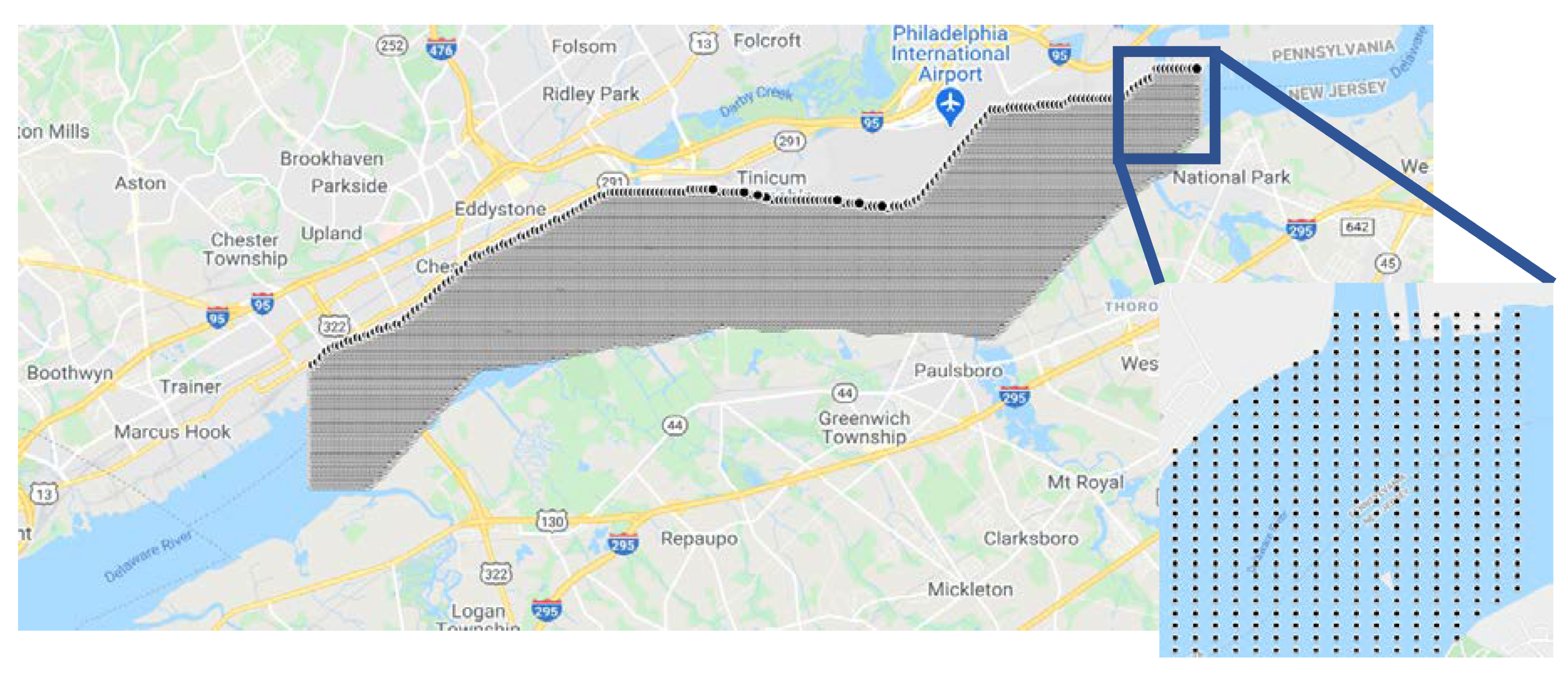
2.1. Definition of the Sampling Grid

While SOSim is a Lagrangian model, fixed on moving patches of sunken oil, a sampling grid is nevertheless imposed on the study area to define points at which bathymetric data are sampled as input to SOSim v2. For an oil spill in an ocean environment, a rectangular sampling grid around the spill location is used. However, considering the complex changes in river shoreline orientation and the small transverse scale of many river environments, a rectangular modeling grid may result in sampling points being defined outside of the river boundary. Therefore, to increase the accuracy of SOSim for use in many navigable rivers, the global Earth topography 5 arc minute (ETOPO5) database of land and seafloor elevations with 1-m resolution is used to create a modeling grid that is representative of the shape of the river. Thus, SOSim is applicable in navigable rivers that flow into oceans, for which the ETOPO5 database has readily available bathymetric information. If there are no bathymetric data in the database for a particular river, such as some areas of the Mississippi River, and the user has access to a bathymetric file or a list of soundings taken with coordinates for the area of interest, SOSim will use the coordinates in the uploaded file as the modeling grid.

To create the new modeling grid using the global database, SOSim first creates a rectangular modeling grid based on the scale defined by the user in the area of interest, consisting of 2000 grid nodes in each direction. SOSim then uses the ETOPO5 database to determine which of those modeling points are bathymetric rather than topographic (e.g., depth below the surface rather than height above surface). All points that are located in the river are kept and used, and all other points are discarded. Figure 1 represents an example of SOSim’s river boundary modeling grid in the Delaware River. Here, a portion of the grid is enlarged to show the grid points (black dots). These dots represent the location of bathymetric data points that are input to the generalized Gaussian conditional sampling distribution for computing the relative oil concentration of the sunken oil. The grid is orthogonal, except along the boundaries of the river. Hence, the grid follows the shape of the Delaware River, closely. Note that the generated boundaries are approximate due to the vertical resolution of the bathymetric database.

The bathymetric sampling grid is defined to ensure that bathymetric data points are not sampled outside of the river boundaries when the user does not have access to a bathymetry file and data are available in the ETOPO5 database. To avoid biasing the model results more heavily on the field observations or prior information, the number of bathymetric data points were originally sampled the same number of times as the field data. However, as the number of field data points are often limited, sampling bathymetry to that degree may not provide a representative sample of the local bathymetry. Therefore, the bathymetric data are sampled ten times more frequently than the field data, and input to ten prior likelihood functions. The tenth root of the product of these likelihood functions is then taken to obtain one representative prior likelihood function.

2.2. Uncertain Parameter Ranges

The default ranges considered in the estimation of model parameters for river spills differ from the default ranges for ocean spills because the transport mechanisms are different. In particular, downstream currents and longitudinal dispersion in rivers are much greater than the transverse currents and dispersion. Typical flow velocities in rivers and streams range from approximately 0.2 to 2.9 knots (8.89 to 128.9 km/d) [25]. Flow velocities are highest at the surface and lowest near the channel bed. In addition, bottom currents may not be able to move the sunken oil in a continuous manner [26,27], due, for example, to the formation of a tar mat on the bottom, as was observed following the storage tank fuel transfer leak in the Detroit River [12] or scoured areas behind objects. Therefore, a common velocity profile and professional judgement were used to estimate default ranges of physically possible values of the sunken oil velocity parameters. Possible ranges of diffusion coefficients for sunken oil were estimated similarly, using well-known longitudinal and transverse diffusion coefficient relationships to estimate bottom diffusion in rivers [25].

Default parameter ranges are shown in

Table 1. Default parameter ranges of the Subsurface Oil Simulator (SOSim) for use in rivers.

Parameter	Units	Minimum	Maximum
$v_x$	km/d	−67.1	67.1
$v_y$	km/d	−2.4	2.4
$D_x$	km2/d	0.01	0.6
$D_y$	km2/d	0.01	0.2
$\rho$	[-]	−0.999	0.999
$\gamma$	[-]	0	1

. These ranges worked well over the course of model development, and can be otherwise specified as needed by the user. Flow velocities in rivers are highly variable. For example, currents in the Mississippi River following the T/B Apex 3508 spill were 1.8 knots (80.01 km/d), but were as high as 8 knots (355.6 km/d) in the river following the Apex Towing spill [9]. In addition, currents in the Detroit River during the storage tank fuel transfer leak were roughly 3 to 4 knots (133.3 to 177.8 km/d), though the bottom currents were not great enough to significantly transport the viscous coal tar [12]. Hence, the user can edit velocity and diffusion parameter ranges to reflect local conditions, based on site-specific data on subsurface currents, turbulence, or forces required to move sunken oil, if available.

2.3. Accounting for Flow along Streamlines

River flow moves along streamlines (constant velocity contours) [28,29], rarely crossing them [29]. Further, because sediment transport is largely controlled by river flow, sunken oil transport can be expected to be influenced by river flow as well, and hence sunken oil droplets or patches are not expected to cross streamlines other than through diffusion, which is expected to be low (Table 1).

To incorporate sunken oil transport along streamlines, a local velocity vector would need to be calculated at each sampling grid point, requiring users to input river velocity data, which may be difficult to obtain during emergency response. Such hydrodynamic data are not accepted as an input to SOSim, and hence streamlines are not directly calculated in the model. Instead, when data are available only on a single date, the inferred diffusion coefficient is fixed at the maximum likelihood value for purposes of forecasting transport with minimal movement across streamlines. When data are available on multiple days, the diffusion coefficient is allowed to change with time based on the data.

2.4. Development of a 1-D Model

For demonstration purposes, SOSim was re-written as a 1-D model and demonstrated versus data collected from a non-navigable area of the Kalamazoo River. This procedure allowed modeling of the spill, because generally tracing the movement of the sunken oil downstream was the key issue. There were also no publicly available bathymetric databases for the Kalamazoo River to utilize in defining the river boundaries, and the limited bathymetric data received from US EPA were insufficient for this purpose. The updated model produced one dimensional distributions of the probability of finding sunken oil along the length of the river. Latitudinal and longitudinal coordinates of the river were then extracted from ArcGIS and used to create the 2-D map of relative oil concentrations. Then, the 1-D probability distribution was plotted as bands of relative oil concentrations along the length of the river. However, this procedure cannot be automated given currently available data.

3. Model Demonstration

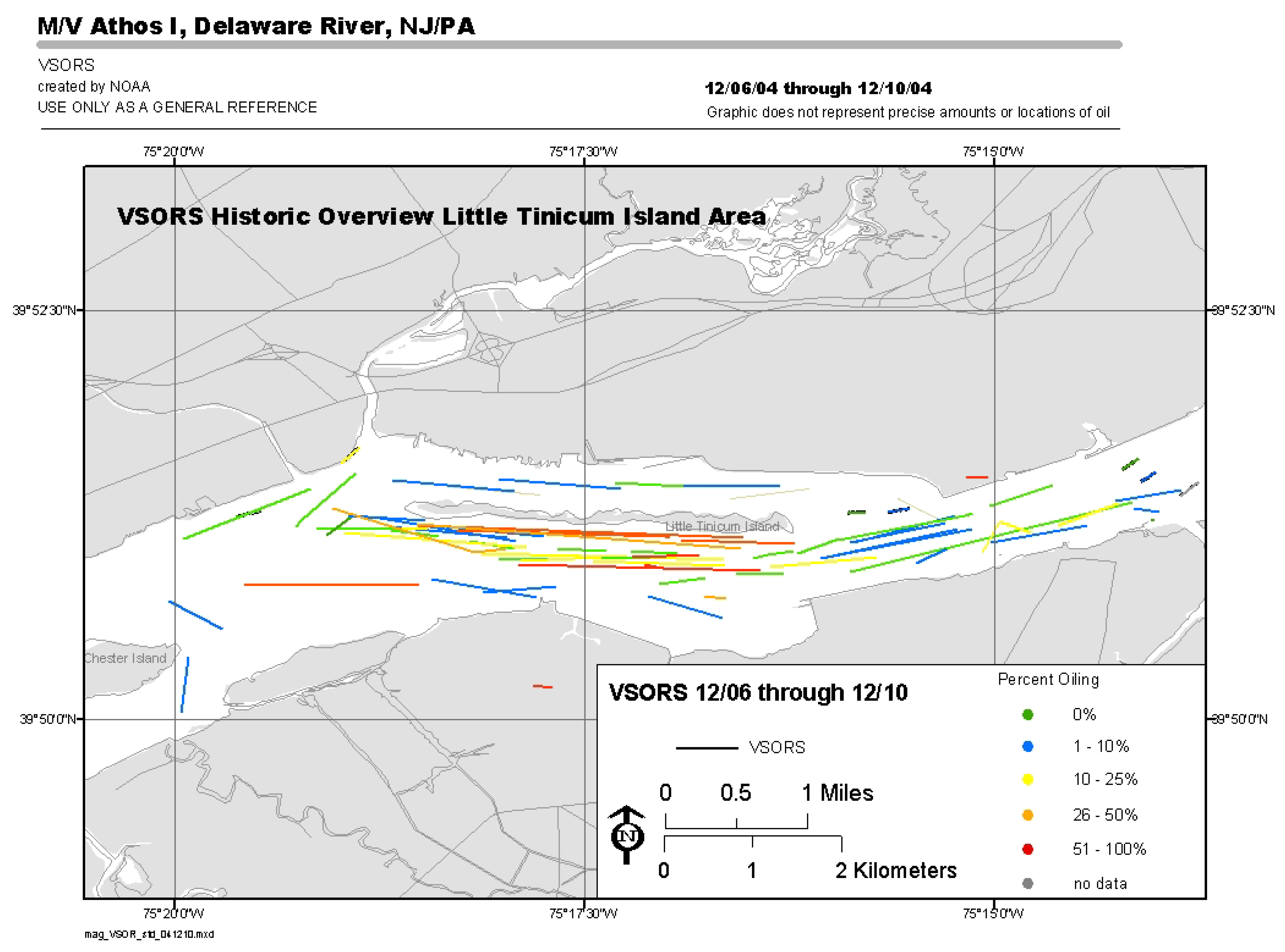
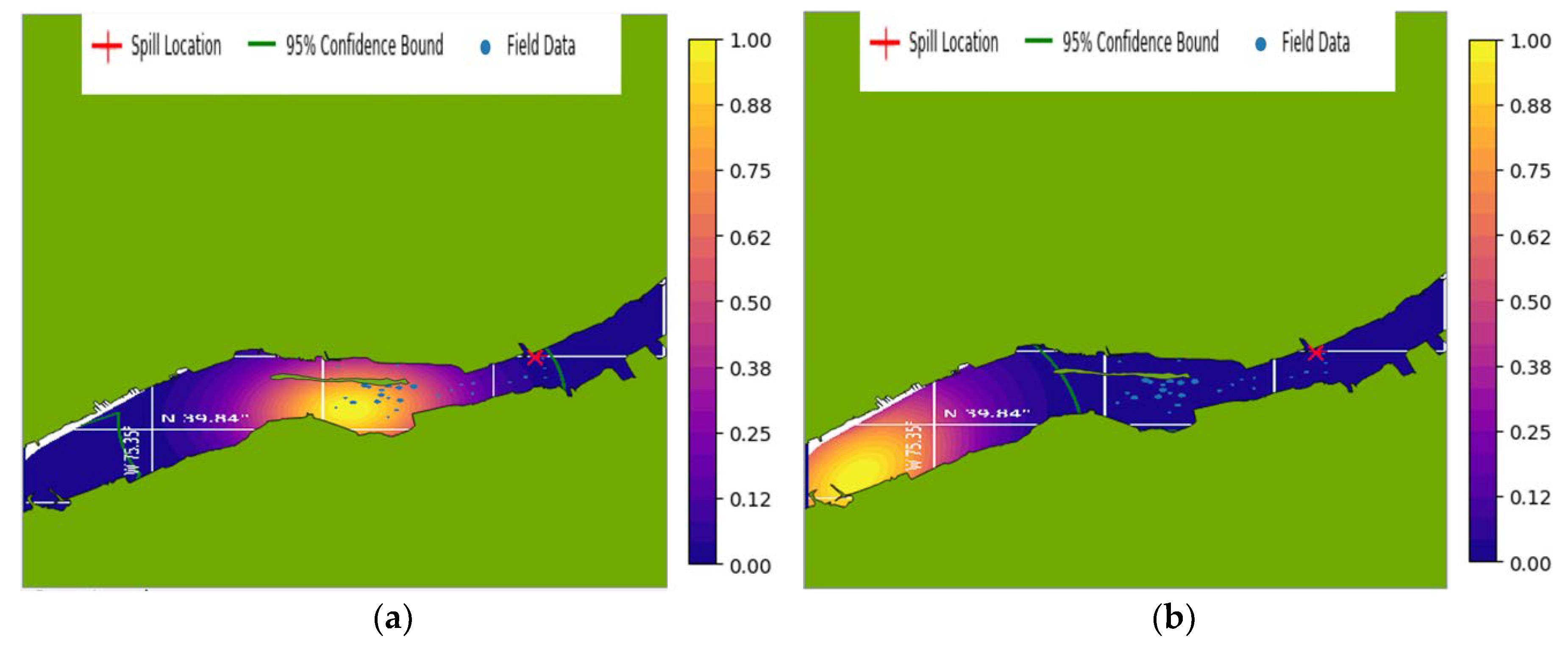
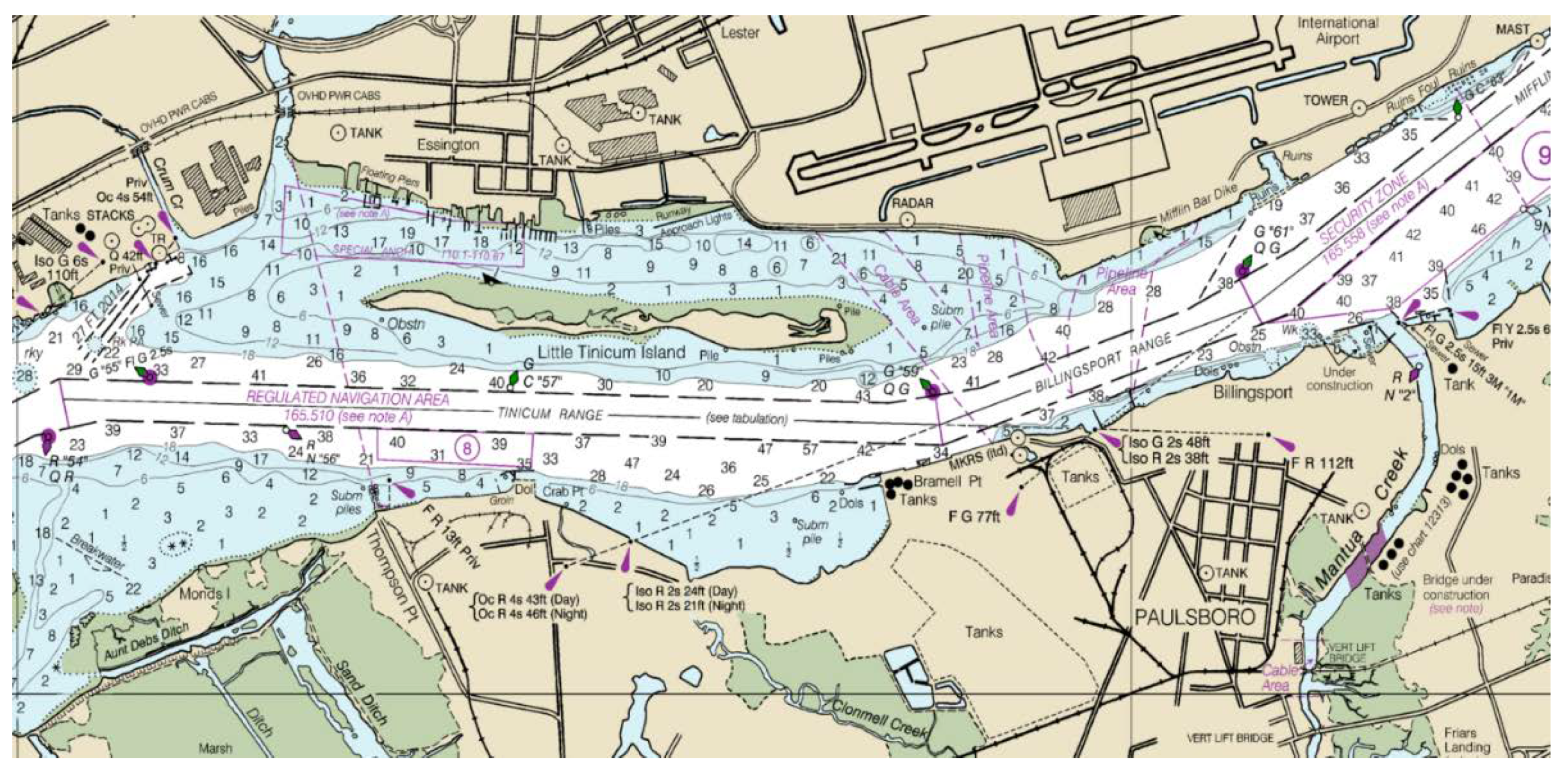
3.1. M/T Athos I Oil Spill

The SOSim v2 sunken oil module was first demonstrated using field data collected after the M/T Athos I oil spill. This spill occurred on 26 November 2004 in the Delaware River near Paulsboro, NJ, USA when the M/T Athos I tanker struck an uncharted submerged object. The collision resulted in a perforation of a ballast tank, causing ~978 metric tons of Bachaquero Venezuelan crude oil with an API gravity of 13.2–13.9 to be released to the river [10]. A small amount of the spilled oil sank due to sediment entrainment. Sunken oil was located in depressions under the collision site and was immobile due to the highly cohesive nature of the oil [10]. In addition, stranded oil in the intertidal zone picked up sediment and sank in the river, and this oil was transported by riverine and tidal currents. Recovery was especially important because the mobile sunken oil threatened intakes to a nearby nuclear power plant and benthic organisms in the area [10].

Vessel Submerged Oil Recovery System (VSORS) field data, collected after the spill, were used as input into SOSim in the form of latitude/longitude coordinates and the respective concentration of oil on the bottom. The field observations were collected from 6 December to 10 December 2004 (Figure 2). The VSORS’ oil sorbent “pom-poms” were dragged along the bottom and recovered to assess the amount of oiling [9]. The resulting field data are shown in Figure 2. Only a portion of these data, representing roughly one half of the study area, were used as input to SOSim to allow demonstration of the model’s ability to locate sunken oil across the entire study area, similar to previous work [21,23]. Several assumptions were made when extracting the data from Figure 2 as input. First, because no specific sampling dates were assigned to each VSORS drag, we assumed that all data were collected on 8 December 2004, the midpoint of the 5-day sampling period, 12 days after the spill. Second, because VSORS data depict only a drag line rather than an exact location of oil on the bottom, the midpoint of each drag was assumed as the sunken oil location for input into SOSim. Lastly, each drag was given a range of percent oiling, so the midpoint of each range for each drag was used as the concentration of sunken oil in the model. These assumptions created significant uncertainty in the model and hence in SOSim’s output. Note also that the data points indicating 0% concentration were also input to SOSim, as inclusion of data points representing no sunken oil will allow SOSim to better infer the location of sunken oil.

Bathymetric data were downloaded from NOAA’s Bathymetric Data Viewer for the area of interest and input to SOSim as one data file. In this demonstration, ten times more bathymetric data points were sampled than the number of available field data points, to obtain a representative sample of the local bathymetry. The tenth root of the product of the prior likelihood functions was then taken to obtain one prior likelihood function, as described in Jacketti et al. [23], to avoid weighting the evidence towards bathymetry and away from field data. The optional inputs and outputs for the M/T Athos I case study are described in

Table 2. Inputs and outputs for demonstration of M/T Athos I oil spill.

Required Input	Output
Spill coordinates and time: 39.86° N, 075.23694° W on 26 November 2004 at 00:00 Field observations: VSORS concentration data Figure 2 (lat/lon, concentration) and Sampling Date (8 December 2004) at 00:00 Desired prediction dates: 8 December 2004 and 20 December 2004	Maps of relative oil concentration (conditional probability)
Optional Input	Optional Output
Bathymetry Data Defined Modeling Area: 0.3° lon × 0.1° lat around the spill Interactive spatial scale and resolution: 2000 grid nodes in each direction	Location of VSORS concentration data 95% confidence bounds

. The scale and resolution were chosen (Table 2), and the default river parameters were used (Table 1). A 95% confidence bound was chosen for display with the field data on a map of the spill site in the Delaware River.

The first SOSim assessment was conducted to locate the full extent of the oil in space on the assumed sampling date. In addition, although forecasts may be less reliable when data are available from only one sampling date, due to uncertainties in the inferred velocity and diffusion coefficients, a second prediction was made 24 days after the spill (12 days after the sampling campaign). This forecast was based on default parameters for the initial advection and dispersion of the oil during settling [23], to test the model’s ability to forecast the movement of sunken oil in a river setting based on limited data. Figure 3a,b represent assessments of the location of sunken oil 12 and 24 days after the initial spill, respectively. The red cross represents the spill location and the green line represents the 95% confidence bound on a 4% concentration of oil. The blue dots represent the field data, with the size of the dot corresponding to the recorded concentration in percent. The assessed relative oil concentrations are normalized from 0 to 1 and are analogous to the relative probability of finding sunken oil at specific locations.

The model results in Figure 3a are realistic in that the initial prediction covers the area for which data indicate the presence of oil were input to the model, as well as the area further to the West, covering all of Tinicum Island, also found to be oiled but for which data were not input to SOSim. The sunken oil patch in Figure 3a is wide and significantly dispersed due to the uncertainties and assumptions in the field data that were input. In addition, the three low-concentration field data points just to the East of the initial spill location are encompassed by the confidence bound. Further, the most concentrated area of the sunken oil patch is located just South of Tinicum Island, within the deepest channel of the river. Figure 4 represents a bathymetric chart for the Delaware River near Tinicum Island. When comparing the most concentrated area in the sunken oil patch in Figure 3a and the bathymetric chart, the most heavily oiled area is located within the channel at roughly 47 feet. Thus, model output based on bathymetric data and field observations were consistent with the observed and expected locations of sunken oil in the Delaware River.

The forecast in Figure 3b is consistent with the downstream currents in the Delaware River. Within three days of the VSORS tows in Figure 2, the amount of sunken oil surrounding Tinicum Island steadily declined [30]. Thus, SOSim’s assessment of the location of sunken oil 12 days after the sampling campaign corresponds with observations after the spill. The sunken oil may have been thought to travel further in 12 days due to the swift river currents, which were roughly 2 knots (88.9 km/d) at the time of the spill [30]. However, the sampled field data were taken 12 days after the initial spill and the majority of the sunken oil was in close proximity to the spill location. In addition, sunken oil will generally move slower than river currents and currents are slower at the bottom due to bottom boundary friction. Overall, SOSim was able to provide realistic 2-D predictions for the movement of sunken oil in the Delaware River. However, more high quality and quantitative field data will allow the model to generate more accurate results that reflect both the observations in the field and the local bathymetry.

The velocity and diffusion parameters inferred by SOSim for the ‘Best Guess’ sunken oil patch (Figure 3a), and the parameters inferred for the confidence bound are shown in

Table 3. SOSim’s inferred velocity and diffusion parameters for M/T Athos I case.

Parameter	Best Guess Patch	Conf. Bound Patch
$v_x$ (km/d)	−0.396	−0.414
$v_y$ (km/d)	−0.136	−0.136
$D_x$ (km2/d)	0.152	0.152
$D_y$ (km2/d)	0.0527	0.0702

. The inferred parameters are well within the range of the default parameter values and suggest the parameter ranges are appropriate.

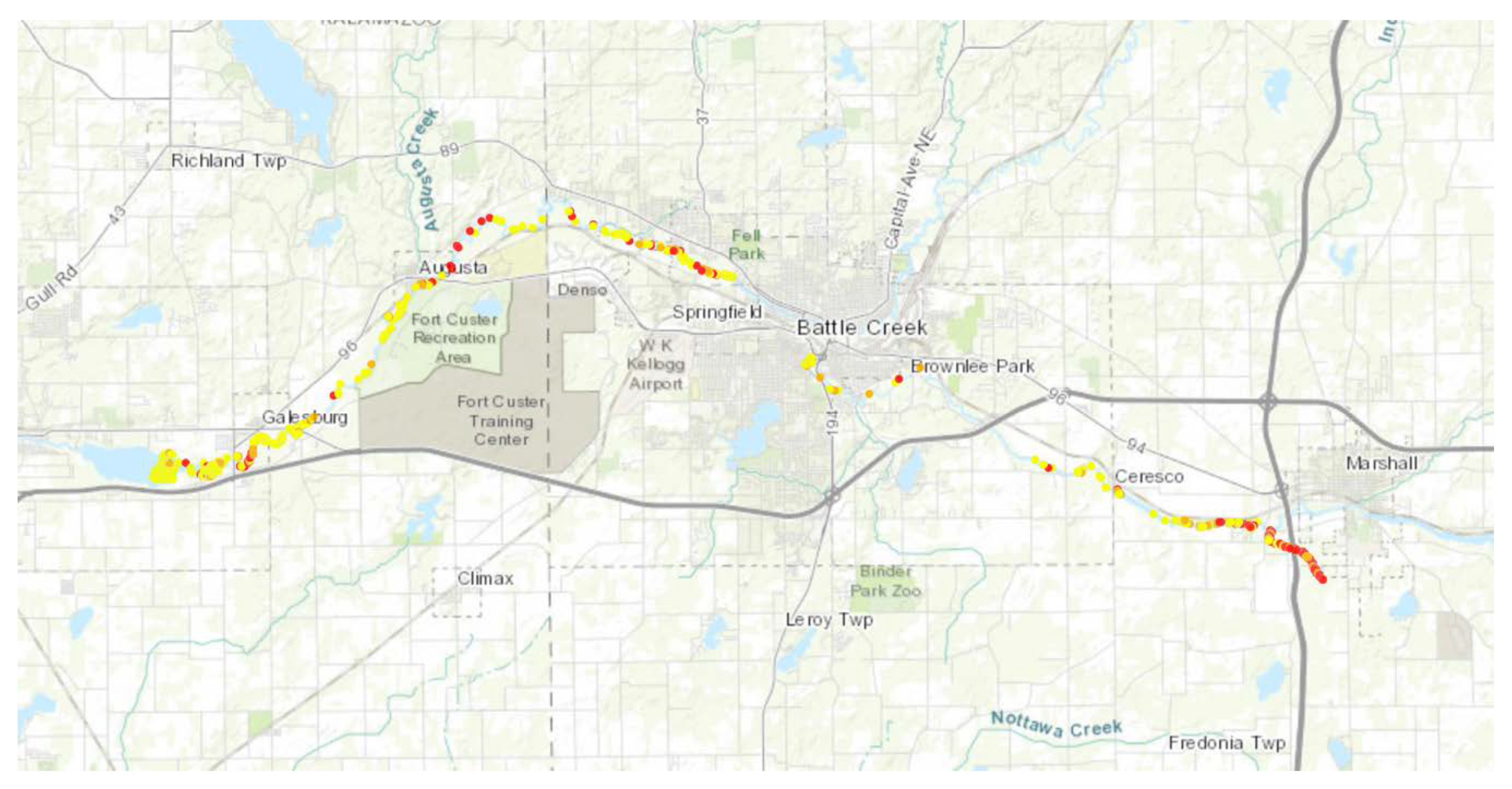
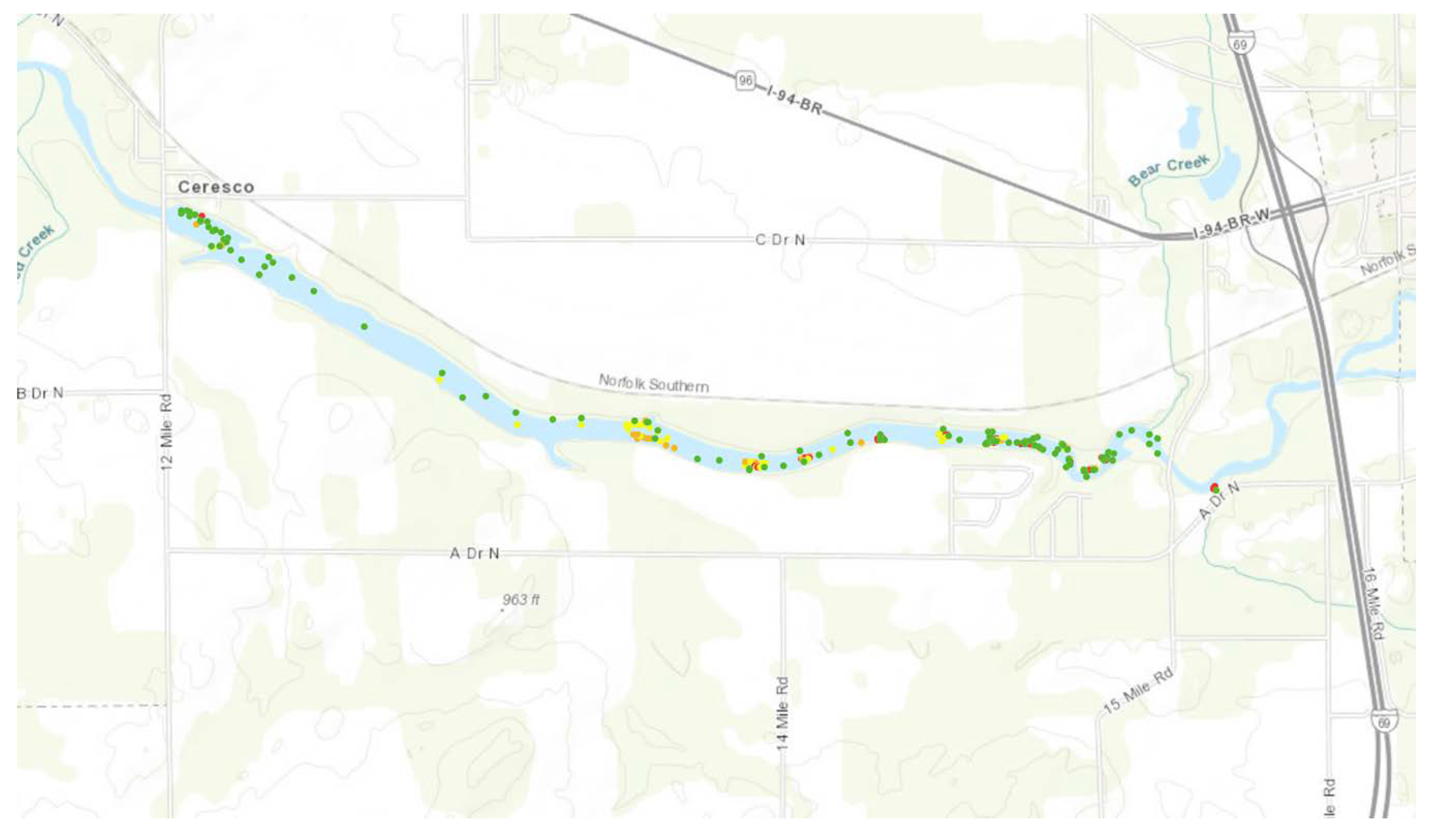
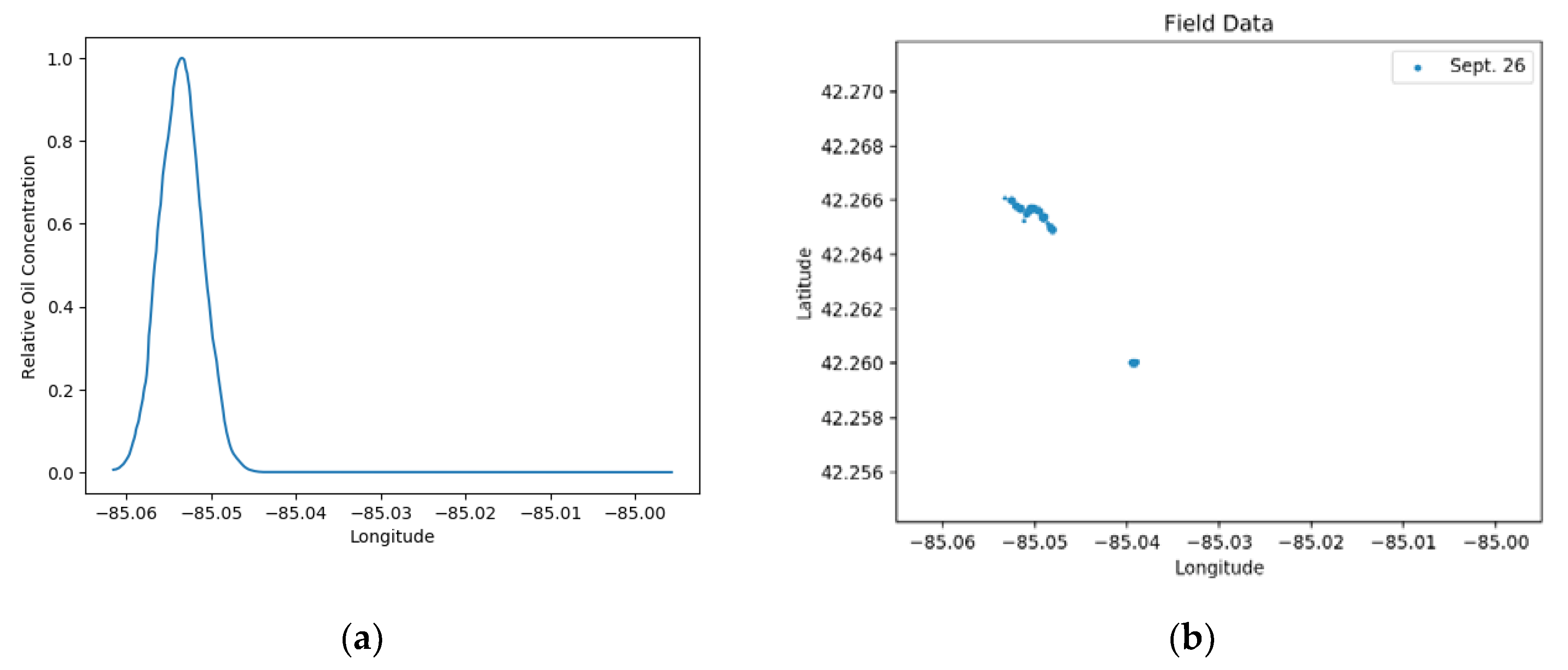
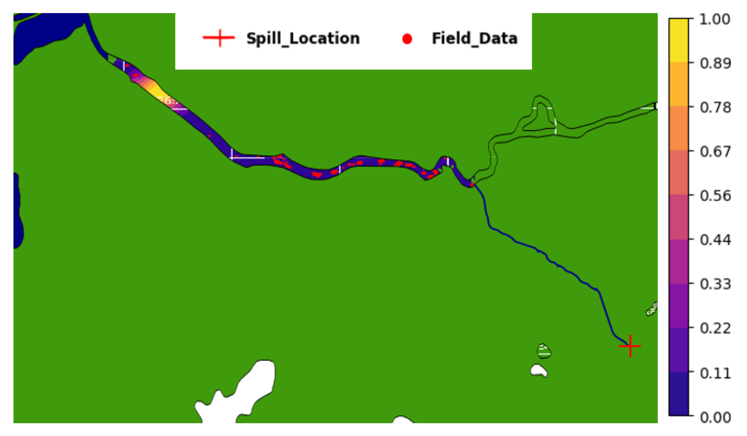
3.2. Enbridge Kalamazoo River Oil Spill

The Enbridge Kalamazoo River oil spill occurred on 26 July 2010 when an Enbridge operated pipeline burst and oil flowed into Talmadge Creek, which feeds into the Kalamazoo River near Marshall, Michigan, U.S.A. The 76 cm ruptured pipeline initially spilled ~3000 metric tons of diluted bitumen (DilBit) [31], resulting in the largest inland river spill in Midwestern U.S. history [13,32]. In this case, the DilBit was floating initially, and once the volatile hydrocarbons evaporated, a portion of the heavier bitumen became submerged in the water column [13]. OPAs were then formed from the submerged bitumen and sank, settled, and re-suspended in different areas along the river [19,33]. Some factors that enhanced the formation of OPAs were the warm water temperatures and increased turbulence and suspended sediments due to floodwater [33]. According to Dollhopf and Durno [13], sunken OPAs were most prevalent in areas where the velocity of the surface water was less.

Following the Enbridge Kalamazoo River oil spill, a poling was used to detect the sunken OPAs [33]. That is, response teams used poles to stir up the sediment on the bottom of the river, recording the presence of sunken oil if a sheen or tar ball floated to the surface or oil adhering to the pole [32]. Poling data throughout the Kalamazoo River from 2010 to 2014 were obtained from the US EPA, starting from 29 August 2010. Poling data are more quantitative than VSORS data, because exact locations with associated sunken oil concentrations are recorded. However, the assessed concentrations are qualitative, listed as “heavy”, “moderate”, “slight”, or no oiling [34]. Therefore, the qualitative concentrations were converted to numerical oil concentrations, ranging from 0–100%.

SOSim was designed first for emergency response, so data from 29 August to 21 September 2010 were extracted and used as input for the initial model run. Figure 5 shows the entirety of the Kalamazoo River that was sampled from 29 August to 21 September and includes the points where sunken oil was observed. Rather than using data along the entire river up to Morrow Lake (roughly 1800 data points), data only from the approximate spill site to the sixth transect were input to the model, to assess impacts to the most heavily oiled section of river (Figure 6). In fact, significant sunken oil was identified in the first 3-km stretch downstream of the spill site by the end of the 3 month pre-recovery poling assessment [20]. All data points along this river segment, including at locations with zero concentration, were input to SOSim.

As a result of no publicly available bathymetric datasets in this area of the Kalamazoo River, the depths of the river were extracted from all of these data points provided by the US EPA and input to SOSim. In addition, SOSim was run in 1-D in space, so the coordinates that were extracted from ArcGIS Pro to create a 2-D output following the river were used as the locations of SOSim model output. Further, the velocity and diffusion parameter ranges were adjusted based on the available field data on subsequent days and the small scale of the area of interest (~7 km). SOSim’s output is a 1-D probability distribution for locating sunken oil in the longitudinal direction. This output is then converted to a 2-D map of relative oil concentrations along the Kalamazoo River to visually assess the highest probability of finding sunken oil in the river. The required and optional inputs and outputs to SOSim are described in

Table 4. Inputs and outputs for demonstration of Enbridge Kalamazoo River oil spill.

Required Input	Output
Spill coordinates and time: 42.2395° N, 084.9662° W on 26 July 2010 at 00:00 Field observations: Poling concentration data Figure 6 (lat/lon, concentration) and Sampling Date (29 August–21 September 2010) at 00:00 Desired prediction date: 26 September 2010	1-D probability distribution of sunken oil location in the x-direction Bands of relative oil concentration (conditional probability)
Optional Input	Optional Output
Bathymetry Data Defined Modeling Area: 0.1° lon around the spill Interactive spatial scale and resolution: 450 grid points	Location of VSORS concentration data

.

SOSim predicted the location of sunken oil along the river 5 days after the last sampling campaign (2 months after the initial spill) to compare the model result with observed data in the area of interest on the same day and demonstrate the model’s ability to predict the movement of sunken oil into the future. Figure 7a represents SOSim’s prediction for the location of sunken oil in 1-D on 26 September 2010. In Figure 7a the forecasted location of sunken oil on 26 September 2010 can be seen. In Figure 7b, the observed sunken oil locations on the same day as the forecast are shown, with the size of the dot corresponding to the concentration of sunken oil. When comparing Figure 7a,b, SOSim was able to predict the longitudinal location of the sunken oil as the same location as the majority of the field observations at roughly 85.05° W. The 1-D result produced by SOSim was then plotted as bands along the Kalamazoo River to give users a visual idea of the location of sunken oil in the river, as shown in Figure 8. The red dots represent the non-zero field data points that were input to SOSim (Figure 6).

4. Discussion and Conclusions

Results presented in this paper indicate that the adaptation of SOSim to also model of spills into rivers, based on Bayesian inference from available field concentration data and bathymetric data, was successful in reflecting the riverine transport mechanisms and scale to delineate areas of higher priority in the search for sunken oil. In particular, results for the M/T Athos I oil spill were consistent with responders’ assessments of the location of sunken oil, using available field observations. According to the Submerged Oil Assessment Unit [30], the greatest concentrations of sunken oil were detected around Tinicum Island soon after the spill, consistent with the patch in Figure 3a. Modeling of the subsurface oil directly after the M/T Athos I spill occurred was used to determine when to safely reopen the water intakes of the Salem Nuclear Power Plant and thus restart power production. Model predictions, however, were based on estimated bottom transport speeds and were later calibrated with observations of sunken oil concentrations [28]. While the modeling results assisted in decision making after the spill, bottom currents are generally not measured and there may be uncertainties in estimating these velocities. The nuclear power plant at the time of the spill was shut down for several days to prevent oil contamination of the circulation and service water intake systems [30], at a total cost of roughly $33.1 million [18], paid for by the Responsible Parties. Hence, a probabilistic model such as SOSim could have been a complement to other model predictions; useful in (1) identifying key sampling locations and (2) predicting when sunken oil would no longer be a threat to the water intake systems, by exploiting field concentration data reflecting system hydrodynamics to estimate oil transport rates and reduce losses.

Smaller, non-navigable rivers pose somewhat different challenges in terms of modeling and response. In that regard, results of the 1-D model adaptation demonstrated versus poling observations following the Enbridge Kalamazoo River oil spill indicate that SOSim is capable of providing forecasts on a small scale utilizing limited available field observations and bathymetric data. Following this spill, a few OPA models were developed and used to hindcast the submerged and sunken OPAs in the Kalamazoo River [19,20,35]. The 1-D model developed by Jones and Garcia [20] simulated the longitudinal distribution of settled particles in the Kalamazoo River and found that almost all of the settled oil was located in the first 1-km stretch downstream of the spill site. Inputs to this model include average river longitudinal, lateral, and vertical velocity components, flowrate, flow depth, and slope, diameter of the river sediments, distribution of oil droplet sizes, and oil density. These input parameters may be difficult to obtain during emergency response compared with field observations and bathymetric data, and thus can influence applicability and accuracy of their model. Both the model by Jones and Garcia [20] and SOSim were able to assess sunken oil concentrations in 1-D within 10 km of the spill site. However, the model by Jones and Garcia [20] does not track an OPA once settled on the bottom.

Overall, the Bayesian SOSim v2 model appears to be an effective tool for tracking slow-moving contaminants such as oil on the bottom of a waterbody, which is growing in importance as heavy oils are being increasingly transported. We can conclude the following based on the results presented in this work:

• Inference based on available field data, and constraints on gravitational deposition, can be an effective approach to forecasting the trajectory of relatively slow-moving pollutant masses, particularly when reliable flow field data are not available;
• even qualitative data on pollutant concentration, such as poling data, are sufficiently informative inputs to an inferential assessment such as implemented in SOSim v2;
• SOSim v2 is applicable for locating and tracking sunken oil in navigable rivers following releases, as long as field observations on sunken oil concentrations and bathymetric data are available; and
• as an open source application, SOSim v2 can be modified to operate in 1-D for non-navigable rivers, at such time as bathymetric data become more widely available, e.g., for definition of river boundaries.

References

1. NOAA; API. Options for Minimizing Environmental Impacts of Freshwater Spill Response; Inland Oil Spills; API Publishing Services: Washington DC, USA, 1994. [Google Scholar]
2. Yapa, P.D.; Tao Shen, H. Modelling river oil spills: A review: Modélisation de déversements de pétrole en rivière: Étatde l’art. J. Hydraul. Res. 1994, 32, 765–782. [Google Scholar] [CrossRef]
3. Hansen, M.E.; Dursteler, E. Pipelines, Rail & Trucks—Cost Benefit Analysis; Strata, 2017; Available online: https://www.strata.org/pdf/2017/pipelines.pdf (accessed on 25 May 2020).
4. National Acadamies of Sciences Engineering Medicine. Spills of Diluted Bitumen from Pipelines: A Comparative Study of Environmental Fate, Effects, and Response; National Acadamies Press: Washington, DC, USA, 2016; ISBN 0309380103. [Google Scholar]
5. Santos, R.G.; Loh, W.; Bannwart, A.C.; Trevisan, O.V. An overview of heavy oil properties and its recovery and transportation methods. Braz. J. Chem. Eng. 2014, 31, 571–590. [Google Scholar] [CrossRef] [Green Version]
6. NOAA. Oil Spills in Rivers. Available online: https://response.restoration.noaa.gov/oil-and-chemical-spills/oil-spills/resources/oil-spills-rivers.html (accessed on 25 May 2020).
7. Fitzpatrick, F.A.; Johnson, R.; Zhu, Z.; Waterman, D.; McCulloch, R.D.; Hayter, E.J.; Garcia, M.H.; Boufadel, M.; Dekker, T.; Soong, D.T.; et al. Integrated Modeling Approach for Fate and Transport of Submerged Oil and Oil-Particle Aggregates in a Freshwater Riverine Environment. In Proceedings of the Joint Federal Interagency Conference, Reno, NV, USA, 19–23 April 2015; pp. 1–12. [Google Scholar]
8. Harper, J.R.; Sergy, G.; Britton, L. uSCAT Technical Reference Manual: Underwater Seabed Cleanup Assessment Technique for Sunken Oil; Coastal and Ocean Resources: Victoria, BC, Canada, 2018. [Google Scholar]
9. API. Sunken Oil Detection and Recovery; API Publishing Services: Washington, DC, USA, 2016. [Google Scholar]
10. Michel, J.; Hansen, K.A. Chapter 13. Sunken and Submerged Oil. In Oil Spill Science and Technology; Gulf Professional Publishing: Houston, TX, USA, 2017; pp. 731–757. ISBN 9780128094136. [Google Scholar]
11. Sawyer, M.; Schweitzer, G.; Davis, A.; Elliott, J.; Mauseth, G.; Scott, T.M. T/B APEX 3508: Best Practices for Detection and Recovery of Sunken Oil. In Proceedings of the International Oil Spill Conference, Long Beach, CA, USA, 15–18 May 2017; pp. 134–155. [Google Scholar]
12. Heiland, R.C.; Smith, B.L.; Hazel, W.E.; Popa, M.; McCarthy, D.J. Underwater recovery of submerged oil during a cold weather response. In Proceedings of the International Oil Spill Conference, Washington, DC, USA, 7–10 April 1997; pp. 765–772. [Google Scholar]
13. Dollhopf, R.; Durno, M. Kalamazoo River\Enbridge Pipeline Spill 2010. In Proceedings of the International Oil Spill Conference, Washington, DC, USA, 23–26 May 2011; p. 422. [Google Scholar]
14. IPIECA. Oil Spills: Inland Response; IOGP Report 514; IPIECA-IOGP: London, UK, 2015. [Google Scholar]
15. NRC. Chapter: 4 Transport and Fate. In Oil Spill Dispersants: Efficacy and Effects; National Academies Press: Washington, DC, USA, 2005; ISBN 030909562X. [Google Scholar]
16. Horn, M.; French McCay, D. Consequence Analysis for Crude-by-Rail Releases into Freshwater Environments. In Proceedings of the 39th AMOP Technical Seminar on Environmental Contaminant and Response, Environment Canada, Ottawa, ON, Canada, 7–9 June 2016; pp. 1–28. [Google Scholar]
17. French McCay, D.P.; Rowe, J.; Crowley, D.; Ducharme, J.; Frediani, M.; Bernardo, M.; Etkin, D.S. Potential Oil Trajectories and Oil Exposure from Hypothetical Spills in the Hudson River. In Proceedings of the 41st AMOP Technical Seminar, Environment and Climate Change Canada, Ottawa, ON, Canada, 2–4 October 2018; pp. 1163–1193. [Google Scholar]
18. NOAA. When the Dynamics of an Oil Spill Shut Down a Nuclear Power Plant. Available online: https://response.restoration.noaa.gov/about/media/when-dynamics-oil-spill-shut-down-nuclear-power-plant.html (accessed on 19 August 2020).
19. Zhu, Z.; Waterman, D.M.; Garcia, M.H. Modeling the transport of oil–particle aggregates resulting from an oil spill in a freshwater environment. Environ. Fluid Mech. 2018, 18, 967–984. [Google Scholar] [CrossRef]
20. Jones, L.; Garcia, M.H. Development of a Rapid Response Riverine Oil-Particle Aggregate Formation, Transport, and Fate Model. J. Environ. Eng. 2018, 144, 1–16. [Google Scholar] [CrossRef]
21. Echavarria-Gregory, M.A.; Englehardt, J.D. A predictive Bayesian data-derived multi-modal Gaussian model ofsunken oil mass. Environ. Model. Softw. 2015, 69, 1–13. [Google Scholar] [CrossRef]
22. Jacketti, M.; Ji, C.; Englehardt, J.D.; Beegle-Krause, C.J. Development of the SOSim Model for Inferential Tracking of Subsurface Oil. In Proceedings of the 42nd (AMOP) Technical Seminar, Environment and Climate Change Canada, Ottowa, ON, Canada, 4–6 June 2019; pp. 485–501. [Google Scholar]
23. Jacketti, M.; Englehardt, J.D.; Beegle-Krause, C.J. Bayesian Sunken Oil Tracking with SOSim v2: Inference from Field and Bathymetric Data. Mar. Pollut. Bull. 2020. under review. [Google Scholar]
24. Broomé, S.; Nilsson, J. Stationary sea surface height anomalies in cyclonic boundary currents: Conservation of potential vorticity and deviations from strict topographic steering. J. Phys. Oceanogr. 2016, 46, 2437–2456. [Google Scholar] [CrossRef]
25. Chin, D.A. Chapter 4: Rivers and Streams. In Water-Quality Engineering in Natural Systems; John Wiley & Sons, Inc.: Hoboken, NJ, USA, 2013; pp. 78–134. [Google Scholar]
26. Beegle-Krause, C.J.; Barker, C.H.; Watabayashi, G.; Lehr, W. Long-Term Transport of Oil from T/B DBL-152: Lessons Learned for Oils Heavier than Seawater. In Proceedings of the Arctic and Marine Oil Pollution Conference 2006, Vancouver, BC, Canada, 6–8 June 2006. [Google Scholar]
27. Boehm, P.D.; Barak, J.E.; Fiest, D.L.; Elskus, A.A. A chemical investigation of the transport and fate of petroleum hydrocarbons in littoral and benthic environments: The Tsesis oil spill. Mar. Environ. Res. 1982, 6, 157–188. [Google Scholar] [CrossRef]
28. Beegle-Krause, C.J. Challenges and Mysteries in Oil Spill Fate and Transport Modeling. In Oil Spill Environmental Forensics Case Studies; Elsevier: Amsterdam, The Netherlands, 2018; pp. 187–199. [Google Scholar]
29. Kindsvater, C.E. Selected Topics of Fluid Mechanics; Geological Survey Water-Supply Paper 1369-A, River Hydraulics; US GPO: Washington, DC, USA, 1958.
30. Submerged Oil Assessment Unit. Submerged Oil Assessment—Athos I Oil Spill; NOAA: Washington, DC, USA, 2004.
31. US EPA Enbridge Spill Response Timeline. Available online: https://www.epa.gov/enbridge-spill-michigan/enbridge-spill-response-timeline (accessed on 27 August 2020).
32. Michigan Department of Community Health. Kalamazoo River/Enbridge Spill: Evaluation of People’s Risk for Health Effects from Contact with the Submerged Oil in the Sediment of the Kalamazoo River; U.S. Department of Health and Human Services: Atlanta, GA, USA, 2012.
33. Fitzpatrick, F.A.; Boufadel, M.C.; Johnson, R.; Lee, K.W.; Graan, T.P.; Bejarano, A.C.; Zhu, Z.; Waterman, D.; Capone, D.M.; Hayter, E.; et al. Oil-Particle Interactions and Submergence from Crude Oil Spills in Marine and Freshwater Environments: Review of the Science and Future Science Needs; U.S. Geological Survey: Reston, VA, USA, 2015.
34. US EPA. FOSC Desk Report for the Enbridge Line 6b Oil Spill in Marshall, Michigan; US EPA: Washington, DC, USA, 2016.
35. Hayter, E.; Mcculloch, R.; Redder, T.; Boufadel, M.; Johnson, R.; Fitzpatrick, F. Modeling the Transport of Oil Particle Aggregates and Mixed Sediment in Surface Waters Environmental Laboratory, ERDC Technical Report; US Army Corps of Engineers: Vicksburg, MS, USA, 2015.
Figure 1. Definition of a grid consistent with river boundaries using the Earth topography 5 arc minute (ETOPO5) database in the Delaware River. The grid is a standard orthogonal grid, except along the boundaries. Map created with Google MyMaps.
Jmse 08 00729 g001
Figure 2. Available Vessel Submerged Oil Recovery System (VSORS) field data collected after the M/T Athos I oil spill. Map created by NOAA [30].
Jmse 08 00729 g002
Figure 3. (a) SOSim’s relative probability of finding sunken oil on 8 December 2004, 12 days after the M/T Athos I spill; (b) SOSim’s relative probability of finding sunken oil on 20 December 2004, 24 days after the M/T Athos I spill. (Cardinal directions in image: North = top, South = bottom, East = right, West = left).
Jmse 08 00729 g003
Figure 4. Bathymetric chart in the Delaware River (NOAA Chart 12312). (Cardinal directions in image: North = top, South = bottom, East = right, West = left).
Jmse 08 00729 g004
Figure 5. Poling data with sunken oil from 29 August–21 September 2010. Created using ArcGIS Pro. The yellow dots correspond to slight oiling, the orange to moderate oiling, and the red to heavy oiling.
Jmse 08 00729 g005
Figure 6. Poling data from 29 August–21 September 2010 input to SOSim. Created using ArcGIS Pro. The green dots correspond to no oiling, the yellow correspond to slight oiling, the orange to moderate oiling, and the red to heavy oiling.
Jmse 08 00729 g006
Figure 7. (a) SOSim’s relative probability of finding sunken oil on 26 September 2010, 2 months after the Enbridge Kalamazoo River spill; (b) location of field observations on 26 September 2010, 2 months after the Enbridge Kalamazoo River spill.
Jmse 08 00729 g007
Figure 8. SOSim’s 1-D model result on 26 September 2010 shown in 2-D along Kalamazoo River. Field data from 29 August to 21 September 2010 that were input to SOSim are shown as red dots.
Jmse 08 00729 g008