Three-Dimensional Fluid–Structure Interaction Case Study on Elastic Beam

Abstract

A three-dimensional T-shaped flexible beam deformation was investigated using model experiments and numerical simulations. In the experiment, a beam was placed in a recirculating water channel with a steady uniform flow in the inlet. A high-speed camera system (HSC) was utilized to record the T-shaped flexible beam deformation in the cross-flow direction. In addition, a two-way fluid-structure interaction (FSI) numerical method was employed to simulate the deformation of the T-shaped flexible beam. A system coupling was used for conjoining the fluid and solid domain. The dynamic mesh method was used for recreating the mesh. After the validation of the three-dimensional numerical T-shaped flexible solid beam with the HSC results, deformation and stress were calculated for different Reynolds numbers. This study exhibited that the deformation of the T-shaped flexible beam increases by nearly 90% when the velocity is changed from 0.25 to 0.35 m/s, whereas deformation of the T-shaped flexible beam decreases by nearly 63% when the velocity is varied from 0.25 to 0.15 m/s.

1. Introduction

Deformation of structures has been an area of interest for engineering. Because the coupling process between fluid and structure plays an important role in many engineering fields. Interaction of fluid and structures in underwater flexible beams is a complex problem in industrial applications. Experimental and numerical research has been conducted to examine fluid–structure interaction (FSI). A number of previous studies are summarized in this section.

Important FSI problems were simulated numerically by Chimakurthi et al. [1]. The authors applied Ansys workbench system coupling and two-way fluid–structure interaction to various multiphysics coupled problems, such as FSI in an oscillating solid structure and sub-sea pipeline vibrations. This study is important, because it shows that Ansys workbench system coupling is highly suited to multiphysics coupled problems. Furthermore, the study results were also validated with other experimental and numerical studies. Gluck et al. [2] studied fluid–structure interaction numerically in different plate forms, such as vertical and L-shaped plates. The authors used two code samples for simulation flow and structure, one using the finite volume method for the flow side and the other using the finite element method for the solid side. The one-way fluid–structure interaction method was employed for the simulation effect of waves on a ship’s hull by Dhavalikar et al. [3]. It was assumed that the ship’s hull was a rigid body and wave loads were then simulated on a rigid body. Narayanan et al. [4] numerically investigated flow behavior past a cylinder with a flexible filament. The commercial software STAR-CCM+ was used for solving the governing equations. Large deformation of a flexible rod in fluid flow was studied numerically and experimentally by Hassani et al. [5]. The authors applied a wind tunnel for testing a flexible rod and a mathematical model was developed by coupling with the Kirchhoff rod theory. The deformation of plants under different combinations of wave periods was examined experimentally by Juan et al. [6]. An oscillatory tunnel and volumetric particle image velocimetry system were used in this study. Results showed the velocity distribution around plants. Mantecon et al. [7] numerically investigated the fluid–structure interaction of nuclear fuel plates under axial flow conditions. The authors employed the commercial software Ansys CFX for modeling the fluid flow and Ansys Mechanical for modeling solid plates. Results showed the maximum deflection of the plates happened at the leading edge. The fluid–structure interaction of a square sail was investigated experimentally and numerically by Ghelardi et al. [8]. Initially, the square sail was tested in a wind tunnel at various velocities and then the ADINA commercial program was applied for numerical simulation under the same conditions. The authors obtained a good overall agreement between experimental and numerical results. Liu et al. [9] studied the FSI of a single flexible cylinder in an axial flow at different inlet velocities. Ansys Fluent commercial software was applied to the flow field. They used a user-defined function (UDF) code sample for the deformation of the cylinder. Results showed that increasing or decreasing vibration depends on flow velocity. Xu et al. [10] applied a new method for solving fluid–structure interaction. The lattice Boltzmann method (LBM) and immersed boundary method (IBM) were combined in this method. The authors used a large-eddy turbulence model (LEM) for high Reynolds numbers. This new method was tested with different benchmarks. The results proved that it has good accuracy. Wang et al. [11] studied three different risers (one steel riser and two composite risers) for their Vortex Induced Vibration (VIV) characteristics using the fluid–structure interaction method. They simulated 2D and 3D models using the Ansys Fluent commercial software. Deformations of the models were obtained. The results show that the displacements of the Fiber Reinforced Polymer (FRP) composite risers are significantly larger than those of other models. The fluid–structure interaction problems of two side-by-side flexible plates were also numerically investigated by Dong et al. [12]. The authors presented results of drag force and energy capture performance in a three-dimensional model. A two-dimensional immersed boundary method was used for simulation fluid–structure interaction of a large structure by Wang et al. [13]. A finite difference method was applied to solve compressible Navier–Stokes equations. The authors validated the results using a flexible plate in a hypersonic flow. Good agreement was found between experimental and numerical data. Turek et al. [14] defined a new benchmark for comparing various methods in fluid–structure interaction problems. They located an elastic object in a laminar incompressible channel flow. A good comparison was obtained in this new benchmark study. Wang et al. [15] investigated the flow past a circular cylinder with a flexible splitter plate. A two-dimensional model was used for simulation of the fluid–structure interaction using two different Reynolds numbers. The authors also studied a circular cylinder with a plate, with a gap between the cylinder and the plate. Zheng et al. [16] used a new fluid–structure interaction method that coupled a finite-element method and immersed boundary method (IBM) to study the flow-induced vibrations of the vocal folds during phonation. Wang et al. [17] presented a fluid–structure interaction (FSI) methodology to simulate flexible submerged vegetation stems and kinetic turbine blades. The structural dynamic solver was based on the combined finite element method–discrete element method (FEM-DEM), and solid and fluid solvers were coupled using an immersed boundary method (IBM) iterative algorithm. The flow solver was a ghost-cell-based sharp-interface immersed boundary method (IBM) described by Mittal et al. [18]. The unsteady, incompressible Navier–Stokes equations were solved and a second-order, central-difference scheme was used for all spatial derivatives. The fluid–structure interaction of a three-dimensional flexible membrane was studied by Nestola et al. [19]. The authors used the immersed boundary method for solving complex structures immersed in laminar, transitional, and turbulent flows. Peskin [20] applied the immersed boundary method to computer simulation of fluid–structure interaction. Eulerian and Lagrangian variables were coupled in this method. A fixed Cartesian mesh for the Eulerian variables and a moving curvilinear mesh for the Lagrangian variables have been used in the immersed boundary (IB) method, particularly in biological fluid dynamics. A monolithic FEM/Multigrid method for the fluid–structure interaction of an incompressible elastic object in laminar incompressible viscous flow was presented by Hron and Turek [21]. Griffith and Luo [22] studied a coupling scheme for the immersed boundary method to link the Lagrangian and Eulerian variables. They used this method for solving FSI problems. The left ventricle of the heart was stimulated by this method. The arbitrary Lagrangian-Eulerian finite element method was applied by Nassiri [23]. They used this method for numerical simulation and experimental investigation of wavy interfacial morphology during high velocity impact welding. Tabatabaei et al. [24] studied the hydrodynamics behavior of an axisymmetric squid model numerically. They applied SST k-w turbulence model for simulation. Various fineness ratios, jet propulsion, and drag force were investigated for different swimming velocities. Squid’s flow characteristics were studied numerically and experimentally by Olcay et al. [25]. Digital particle image velocimetry (DPIV) was used for obtaining velocity contours in the experimental region. Ansys Fluent commercial software was applied for solving governing equations in the flow field. They showed that numerical results were so close to the experimental data. Hydrodynamic forces of a moving cylinder and fixed cylinder were investigated numerically by Eren et al. [26]. They used the dynamic mesh method for recreating mesh and moving a cylinder in the incompressible flow.

To improve our understanding of fluid–structure interaction methodology for flow past a flexible beam, we studied the fluid–structure interaction experimentally and numerically for a single flexible beam. We use a high-speed camera system (HSC) for obtaining the deformation of the beam. The three-dimensional flexible beam model was then investigated numerically at three different velocities. Two-way FSI method was applied for numerical simulation, and also, a validation test was carried out. All in all, this study helps to improve our understanding of flexible beams deformations. The paper was organized as follows: Section 2 defines experimental setup, computational domain governing equations, and numerical methods. Section 3 presents validation of deformation T-shaped flexible beam, numerical results, and discussions. Section 4 contains the conclusions.

2. Materials and Methods

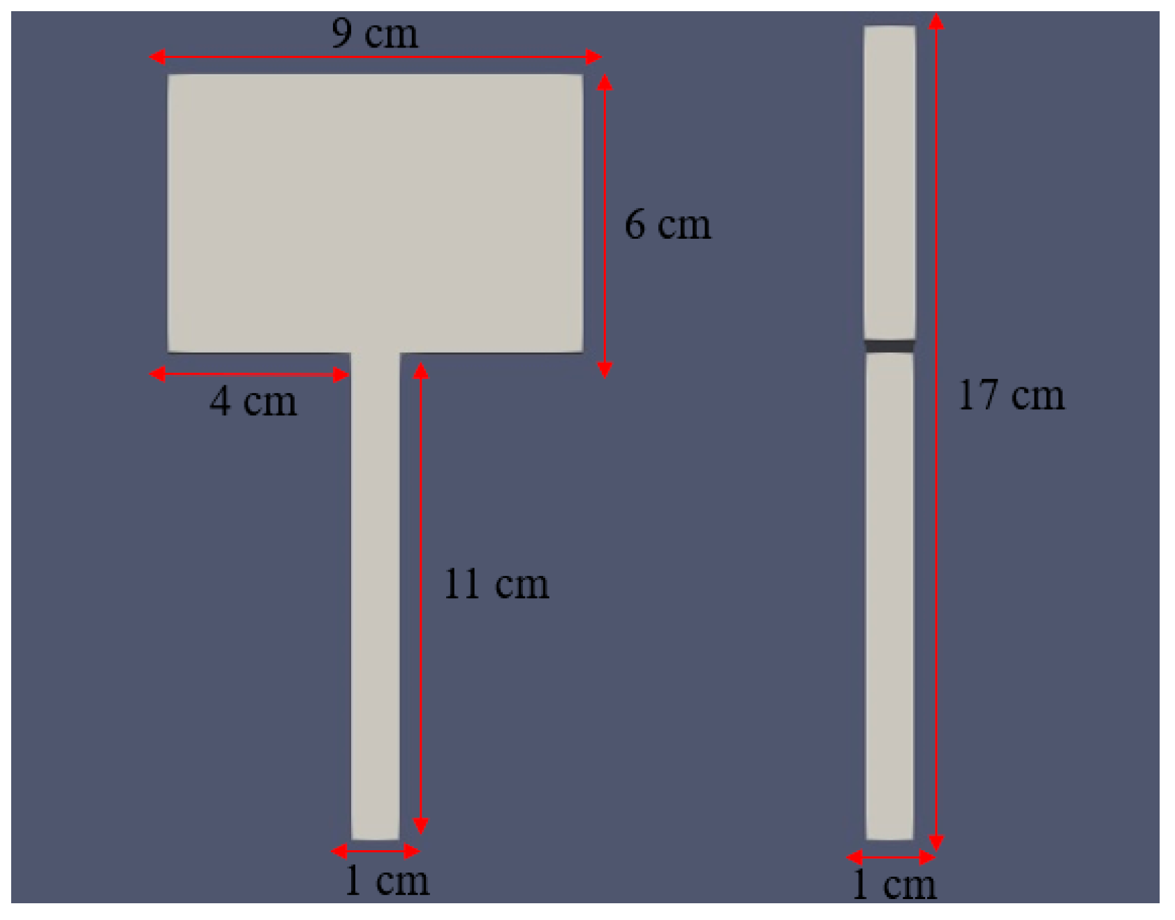
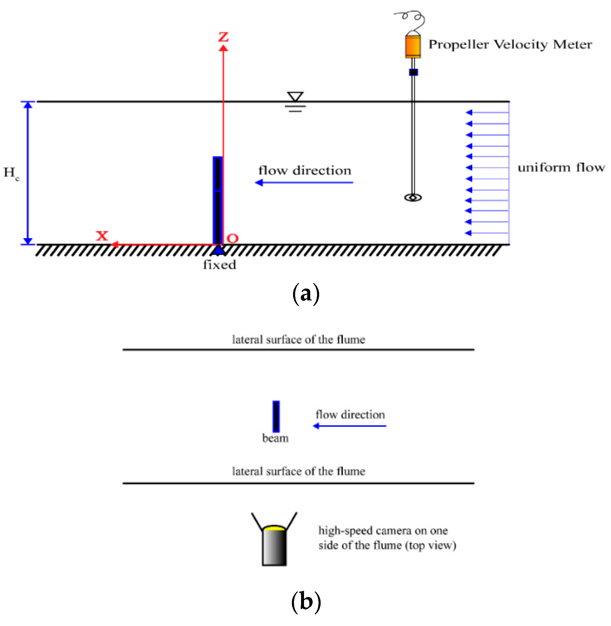
2.1. Experimental Arrangement and Analysis Methodology

Details of the experimental setup are explained in Section 2.2 and Section 2.3. Section 2.2 presents the water channel, the high-speed camera, and the technique of high-speed imaging method. Section 2.3 describes the data analysis of the experiment results.

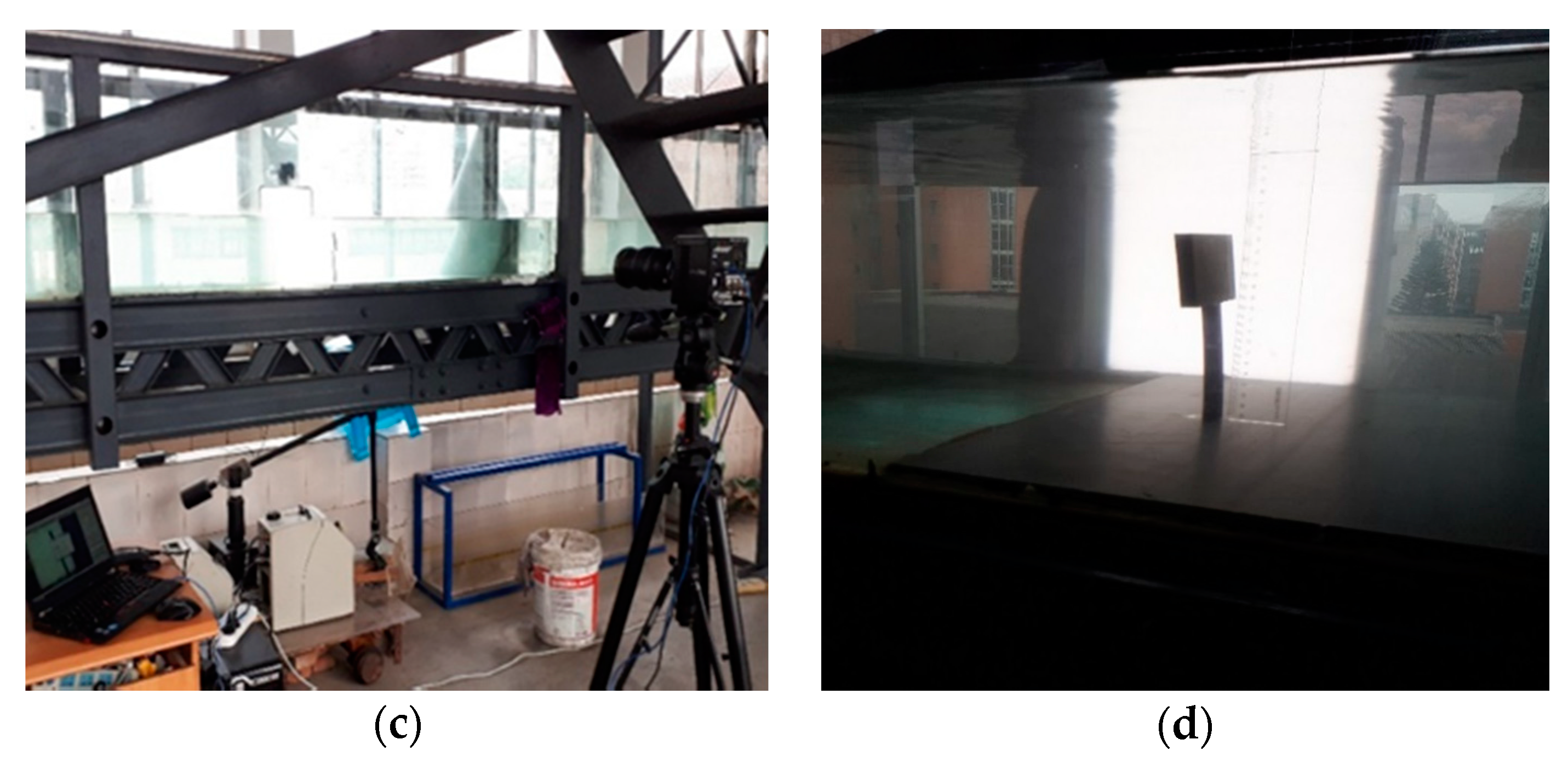
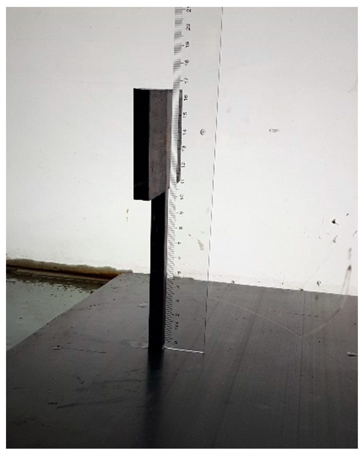
2.2. Experimental Setup

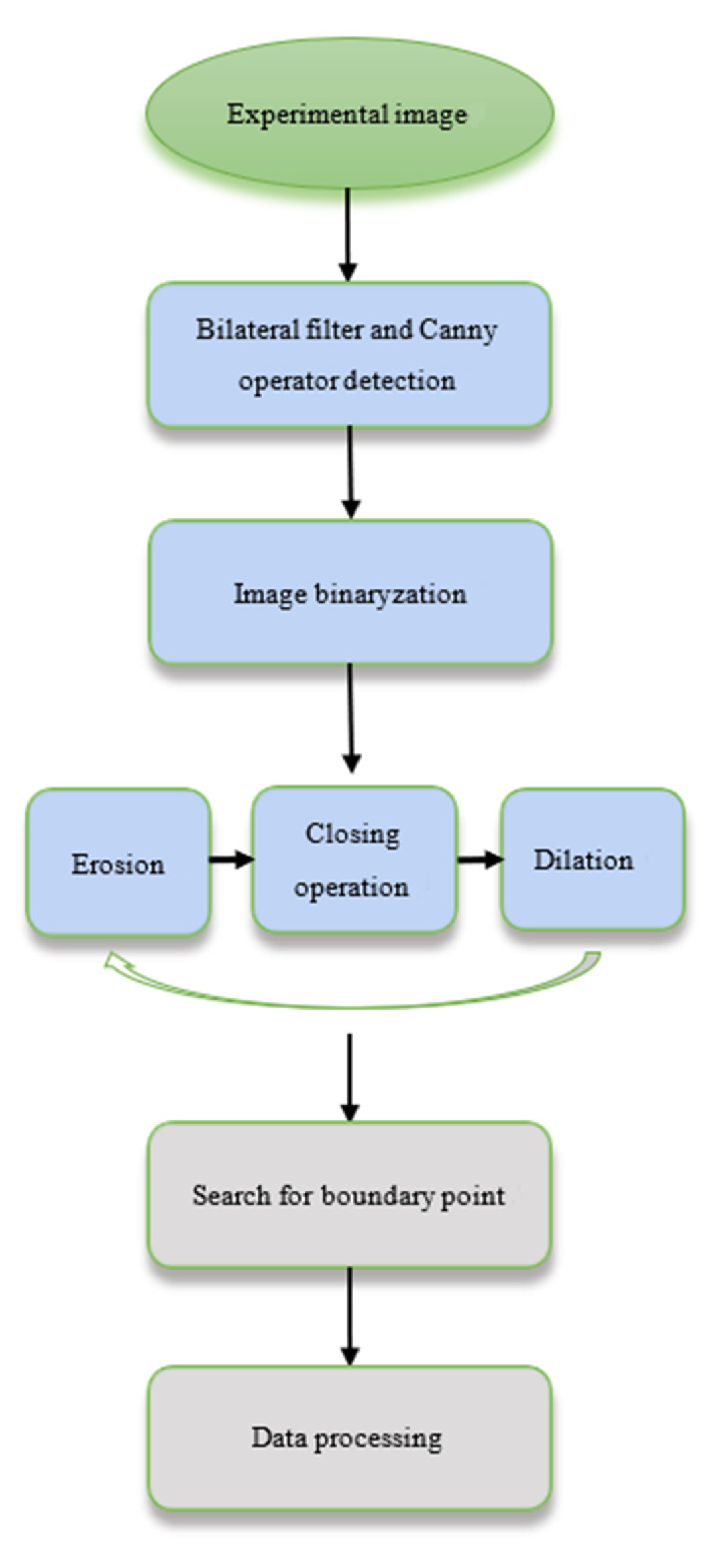
Experiments were carried out in a recirculating water channel of State Key Laboratory of Hydraulics and Mountain River Engineering (SKLHMRE) at Sichuan University (SCU), China. The water channel has a 12 m (length) × 0.5 m (width) × 0.6 m (height) test section with the mean flow velocity up to 0.25 m/s. The water level was maintained at 0.5 m during the experiments and a propeller velocity meter was used to measure the inflow velocity. Froude number is 0.11 (Fr = 0.11), so flow is subcritical in this study. Multiple measurement points in the same vertical plane of the channel at different depths are chosen to measure the velocity in a long period, and the mean flow velocity is calculated by time averaging and space averaging. A T-shaped flexible beam made of polyurethane was fixed in a vertical plane facing to the approaching flow. The dimensions of the T-shaped flexible beam are shown in Figure 1. Water was used for the fluid part and a polyurethane beam was applied for the solid part. The experiment was conducted indoors; physically essential properties of selected materials at room temperature are provided in

Table 1. Characteristics of fluid and solid in numerical and experiment methods.

Water
Density (ρ)	1000 kg/m3
Dynamic viscosity (µ)	0.001 kg/m−s
Flexible Beam
Density (ρs)	1.17 g/cm3
Young’s modulus (E)	18 MPa
Poisson’s ratio (ν)	0.3

.

For the beam motion and image recognition process, illumination was provided by an LED light sheet, and the beam was marked black. A non-intrusive technique of high-speed imaging method was employed to record the deformation of the flexible beam in this study. Images were captured at 1000 frames per second (fps) using a high-speed camera (Fastcam Mini UX100, Photron Inc., Chiyoda-Ku, Tokyo, Japan, maximum acquisition rate: 4000 fps with the resolution of 1280 × 1024 pixels). The resolution of the images is cut down to 616 pixels × 1024 pixels for saving camera memory space to only cover the area where the beam exists, as shown in Figure 2.

The standardization tests were carried out in still water in order to determine the actual distance per pixel (Figure 3). The field of view was approximately 12.07 cm × 20.07 cm, leading to a spatial resolution of 0.0196 cm pixel⁻¹.

2.3. Data Analysis

To track the deformation of the T-shaped flexible beam, an image recognition Python code was developed to obtain quantitative data from images captured in the experiment (Figure 4). A bilateral filter is a basic theory of image noise reduction, and it is better in edge-preserving than other filters, so we used a bilateral filter to reduce the noise of experimental images. Then, the Canny edge detector, which is an edge detection operator that uses a multi-stage algorithm, was used to detect edges of the beam in experimental images. Image binarization was set the grayscale value of the pixel on the image to 0 or 255, which is the process of presenting the whole image with an obvious black and white effect. The erosion, closing operation, and dilation are the morphological operations to enhance image features. We used erosion, closing operation, and dilation to make the edges detected by the Canny edge detector clearer, then the pixel coordinates of the edges were recorded. The pixel size of a picture can be detected. Thus, the scale S of actual distance and Pixel distance can be calculated through Figure 3. S is defined by S = actual distance/pixel distance. Therefore, the actual displacement D of the tracking point is calculated by D = S*L, where L is the pixel distance between the current and initial position of the tracking point. Details about image processing are illustrated in Howes [27].

2.4. Numerical Methods

The two-way fluid-structure interaction (FSI) numerical method is explained in Section 2.5, Section 2.6, Section 2.7 and Section 2.8. The solution of the three-dimensional fluid domain is described in Section 2.5. The structural dynamics of the T-shaped flexible beam is explained in Section 2.6. Section 2.7 presents system coupling between fluid and solid domain. Details of the computational domain and boundary conditions are investigated in Section 2.8.

2.5. Computational Fluid Dynamics (CFD)

The realizable k-ε turbulence model was applied for the turbulent flow simulation in the three-dimensional fluid domain (Olcay et al. [28] and ANSYS Fluent Theory Guide [29]). The governing equations representing the continuity and momentum formulas as given below:

$$\frac{\partial \rho }{\partial t}+\frac{\partial \left(\rho u_i\right)}{\partial x_i}=0$$

(1)

$$\frac{\partial \left(\rho u_i\right)}{\partial t}+\frac{\partial \left(\rho u_i{u}_j\right)}{\partial x_j}=-\frac{\partial P}{\partial x_i}+\rho g_i+\frac{\partial }{\partial x_j}\left(\mu +{\mu }_t\right)\left(\frac{\partial u_i}{\partial x_j}+\frac{\partial u_j}{\partial x_i}\right)+S_i$$

(2)

where $\rho$ is the density and $u_i\mathrm{and}{u}_j$ are the average velocity component of the fluid. P is pressure, $S_i$ is the source term for the momentum equation $\mu$ is the dynamic viscosity, ${\mu }_t$ is the eddy viscosity, and it is defined as ${\mu }_t=\rho C_{\mu }\frac{k^2}{\epsilon }$. The transport equation for $k\mathrm{and}\epsilon$ are for the realizable k − ε model given as,

$$\frac{\partial }{\partial t}\left(\rho k\right)+\frac{\partial }{\partial x_i}\left({\rho ku}_i\right)=\frac{\partial }{\partial x_j}\left[\left(\mu +\frac{{\mu }_t}{{\sigma }_k}\right)\frac{\partial k}{\partial x_j}\right]+G_k+G_b-\rho \epsilon -Y_M+S_k$$

(3)

$$\frac{\partial }{\partial t}\left(\rho \epsilon \right)+\frac{\partial }{\partial x_i}\left(\rho \epsilon u_i\right)=\frac{\partial }{\partial x_j}\left[\left(\mu +\frac{{\mu }_t}{{\sigma }_{\epsilon }}\right)\frac{\partial \epsilon }{\partial x_j}\right]+C_{1\epsilon }\frac{\epsilon }{k}(G_k+C_{3\epsilon }{G}_b)-C_{2\epsilon }\rho \frac{{\epsilon }^2}{k}+S_{\epsilon }$$

(4)

where k is the turbulent kinetic energy and ε is rate of dissipation. $G_k$ is turbulent kinetic energy generation because of the mean velocity gradients, $G_b$ is turbulent kinetic energy generation because of buoyancy, and $Y_M$ is fluctuating dilatation contribution to the overall dissipation rate. The model constants for realizable k-ε turbulence model are $C_{1\epsilon }=1.44$, $C_{2\epsilon }=1.92$, ${\sigma }_k=1.0$, $C_{\mu }=0.09$, and ${\sigma }_{\epsilon }=1.3$.

2.6. Computational Structural Dynamics (CSD)

Deformation of a three-dimensional flexible solid structure is described by the equation of motion, which can be expressed as follows:

$$\left[\mathrm{M}\right]\left\{\ddot{u}\right\}+\left[\mathrm{C}\right]\left\{\dot{u}\right\}+\left[\mathrm{K}\right]\left\{u\right\}=\left\{F\right\}$$

(5)

where [M] is the structural mass matrix, [C] is the structural damping matrix, [K] is the structural stiffness matrix, and $\left\{F\right\}$ is the applied load vector acting on the structure caused by fluid. $\left\{\ddot{u}\right\}$ is the nodal acceleration vector, $\left\{\dot{u}\right\}$ is the nodal velocity vector, and $\left\{u\right\}$ is the nodal displacement vector. Newmark time integration method with an improved algorithm (HHT) was used for the solution of Equation (5). The Newmark method and HHT method were applied for implicit transient analyses. The Newmark method applies finite-difference expansions in the time interval $\Delta t$. It is presumed that (Bathe [30]):

$$\left\{{\dot{u}}_{n+1}\right\}=\left\{{\dot{u}}_n\right\}+\left[\left(1-\delta \right)\left\{{\ddot{u}}_n\right\}+\delta \left\{{\ddot{u}}_{n+1}\right\}\right]\Delta t$$

(6)

$$\left\{u_{n+1}\right\}=\left\{u_n\right\}+\left\{u_n\right\}\Delta t+\left[\left(\frac{1}{2}-\alpha \right)\left\{{\ddot{u}}_n\right\}+\alpha \left\{{\ddot{u}}_{n+1}\right\}\right]\Delta t^2$$

(7)

where $\alpha \mathrm{and}\delta$ are Newmark integration parameters, $\Delta t$ is $t_{n+1}-t_n$, $\left\{u_n\right\}$ is the nodal displacement vector at time $t_n$, $\left\{{\dot{u}}_n\right\}$ is the nodal velocity vector at time $t_n$, $\left\{{\ddot{u}}_n\right\}$ is the nodal acceleration vector at time $t_n$, $\left\{{\ddot{u}}_{n+1}\right\}$ is the nodal acceleration vector at time $t_{n+1}$, $\left\{{\dot{u}}_{n+1}\right\}$ is the nodal velocity vector at time $t_{n+1}$, and $\left\{u_{n+1}\right\}$ is the nodal displacement vector at time $t_{n+1}$.

Since the primary aim is the calculation of displacement $\left\{u_{n+1}\right\}$, the governing Equation (5) can be computed at time $t_{n+1}$ as:

$$\left[\mathrm{M}\right]\left\{{\ddot{u}}_{n+1}\right\}+\left[\mathrm{C}\right]\left\{{\dot{u}}_{n+1}\right\}+\left[\mathrm{K}\right]\left\{u_{n+1}\right\}=\left\{F\right\}$$

(8)

The solution of displacement at time $t_{n+1}$ can be obtained by first rearranging Equations (6) and (7), such that:

$$\left\{{\ddot{u}}_{n+1}\right\}=a_0\left(\left\{u_{n+1}\right\}-\left\{u_n\right\}\right)-a_2\left\{{\dot{u}}_n\right\}-a_3\left\{{\ddot{u}}_n\right\}$$

(9)

$$\left\{{\dot{u}}_{n+1}\right\}=\left\{{\dot{u}}_n\right\}+a_6\left\{{\ddot{u}}_n\right\}+a_7\left\{{\ddot{u}}_{n+1}\right\}$$

(10)

where $a_0=\frac{1}{\alpha \Delta t^2}$, $a_2=\frac{1}{\alpha \Delta t}$, $a_3=\frac{1}{2\alpha }-1$, $a_6=\Delta t\left(1-\delta \right)$, $a_7=\delta \Delta t$.

Once a solution is obtained for $\left\{u_{n+1}\right\}$, velocities and accelerations are computed as defined Equations (9) and (10). For the nodes where the velocity or the acceleration is obtained, a displacement constraint is computed from Equation (7). The HHT time integration method can help to have the desired property for the numerical damping in the full transient analysis (Chung and Hulbert [31]).

The basic form of the HHT method is defined as Equation (11)

$$\left[\mathrm{M}\right]\left\{{\ddot{u}}_{n+1-{\alpha }_m}\right\}+\left[\mathrm{C}\right]\left\{{\dot{u}}_{n+1-{\alpha }_f}\right\}+\left[\mathrm{K}\right]\left\{u_{n+1-{\alpha }_f}\right\}=\left\{F_{n+1-{\alpha }_f}\right\}$$

(11)

where ${\alpha }_m\mathrm{and}{\alpha }_f$ are two extra integration parameters for the interpolation of the acceleration and the displacement, velocity, and loads. It was also realized that the transient dynamic equilibrium equation considered in the HHT method is a linear combination of two successive time steps of n and n + 1 after comparing Equations (5) and (11).

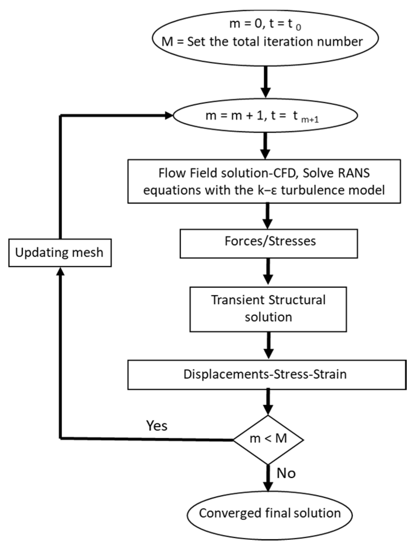
2.7. CFD-CSD Coupling

We used Ansys Workbench-system coupling for simulation two-way fluid–structure interactions (Chimakurthi et al. [1]). Fluid Flow (Ansys Fluent) and the Transient Structural systems (Ansys Mechanical) are connected in system coupling. Reynolds-averaged Navier-Stokes (RANS) equations with the realizable k-ε turbulence model are solved in the computational domain by using the CFD solver (Fluent), and also, transient structural analysis is used to solve the T-shaped flexible beam deformation under the action of loads. Forces or stresses on the fluid side of the interface are transformed on to the solid side, and also, displacements or velocities on the solid side of the interface are transformed on to the fluid side in the system coupling method. Transferring in this system coupling includes the computation of weights and their subsequent use in the interpolation of data. It can happen between topologically similar and/or dissimilar element types, distributions, and dimensions such as surface to surface, volume to volume, point to volume, surface to volume, and vice-versa. Figure 5 shows the calculation procedure and detailed overview of the partitioned system coupling. The induced force on the beam was obtained after the flow field was calculated by using CFD solver from Ansys Fluent. Then, the displacement of the beam was solved by using a structure transient from Ansys Mechanical. This process gets continued until convergence is obtained in system coupling.

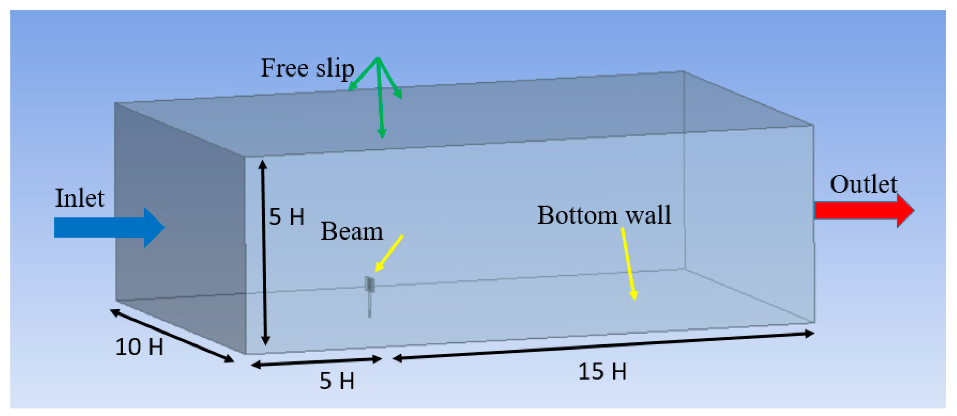
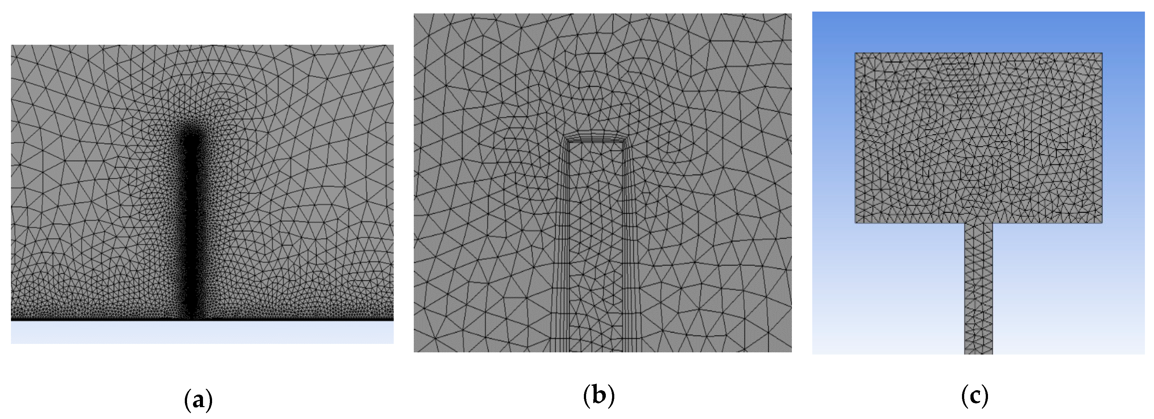
2.8. Computational Model Geometry, Boundary Conditions, and Meshing

The T-shaped flexible beam was fixed on the channel bottom wall. Figure 6 shows the computational domain and boundary conditions schematically. The height (H) of the T-shaped flexible beam is 0.17 m. The beam was put on a cuboid-shape computational domain. The height, length, and width of the domain were defined as 5 H, 20 H, and 10 H. The velocity inlet boundary condition was located at 5H upstream of the beam, and the pressure outlet boundary condition was located at 15 H downstream of the T-shaped flexible beam. No slip boundary condition was selected for walls (bottom wall and T-shaped flexible beam). Free slip boundary condition was applied for top and to the sides of the computational. Dimensions and material properties of T-shaped flexible beam and flow properties that were used in all simulations were the same with experiment case Table 1.

The non-dimensional Reynolds number was applied for defining flow characteristics in this study. The Reynolds number was defined as Equation (12)

$$Re=\frac{\rho UL}{\mu }$$

(12)

where $\rho$ is density, µ dynamic viscosity of the fluid, $U$ free stream velocity, and L is the characteristic length (i.e., height of beam). The highest water velocity was 0.25 m/s in the experimental setup, because the close-circuit water channel could supply 0.25 m/s as the highest water velocity throughout the channel. In the numerical study, three different velocities were used for the understanding of beam behaviors in various velocities. U = 0.15, 0.25, and 0.35 m/s were chosen for numerical simulations after validation. The Reynolds numbers were defined as 25,500, 42,500, and 59,500 for U = 0.15, 0.25, and 0.35 m/s

Table 2. Shows the relation between velocities and applied models.

Velocity (m/s)	Reynolds Number	Applied
0.15	25,500	Numerical model
0.25	42,500	Numerical and experimental model
0.35	59,500	Numerical model

. Commercial computational fluid dynamic (CFD) code Ansys Fluent and Ansys Mechanical programs were employed to solve the flow domain and solid part. A system coupling method was used to connect between flow domain and solid part. The coupled scheme was selected among five pressure–velocity coupling algorithms. The second-order upwind scheme was used for discretization of advective terms of the transport equations. Criteria of convergence were set to 10⁻⁶ for the continuity and momentum equations. The solution of continuity and momentum equations were continued until criteria of convergence were achieved.

Tetrahedron and prism with triangle base elements were set for meshing the fluid solution domain with high-density mesh near walls, and Tetrahedron mesh was used for the solid domain. The dynamic mesh method was applied to simulate the deformation of the T-shaped flexible beam. Totally 800,000–1,200,000 elements were employed to solve the fluid domain, and 21,210–73,000 elements were used to solve the solid domain, as illustrated in Figure 7. A mesh sensitivity study was also carried out for all models in the fluid domain.

Table 3. Mesh convergence study for the computational domain.

Mesh Resolution	Deformation at t = 10 s
810,000	0.022400
890,000	0.01989
920,000	0.01934
1,020,000	0.019147
1,040,000	0.019144

shows the variety of total deformation along with the various number of elements at 0.25 m/s inlet velocity. It was identified that 1,200,000 elements for the fluid solution domain, and 72,425 elements for the solid domain were needed for obtaining good results at maximum velocity in our study. Three different coupling time steps were inspected at 0.01, 0.001, and 0.0001. All simulations were run for a total time of 10 s in this study. A time step of 0.001 was selected for all simulations after mesh refinement studies.

3. Results and Discussion

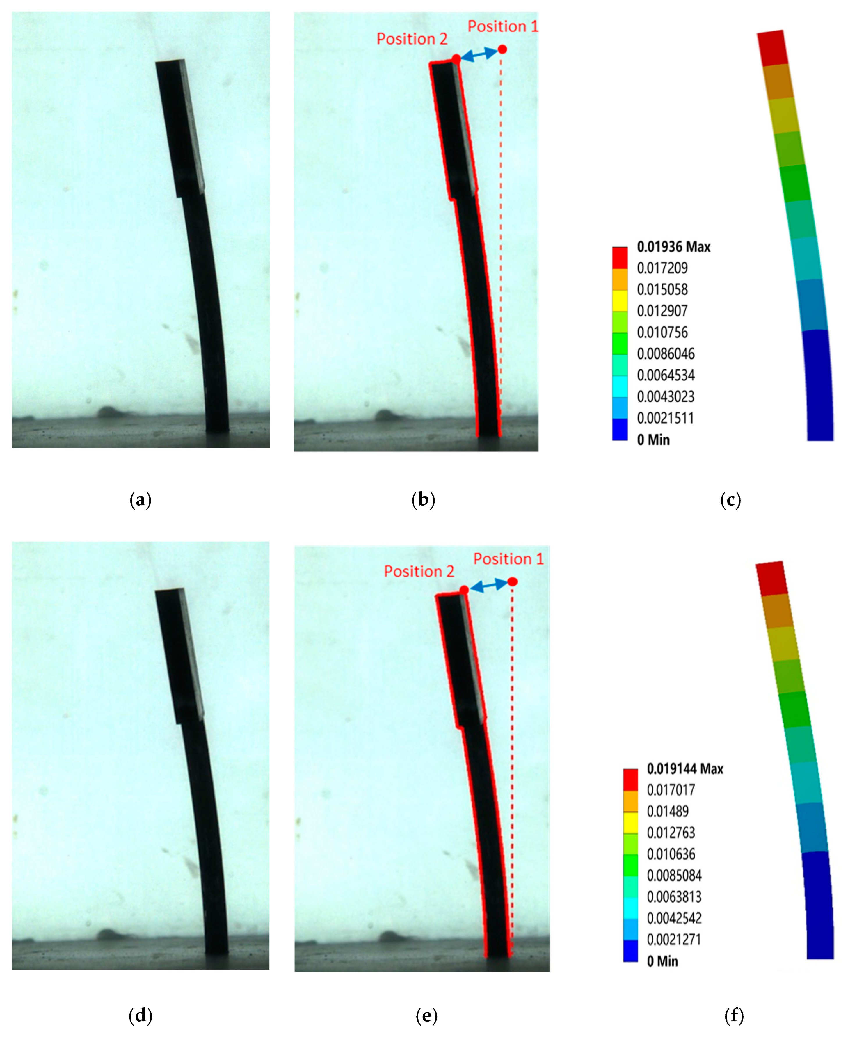
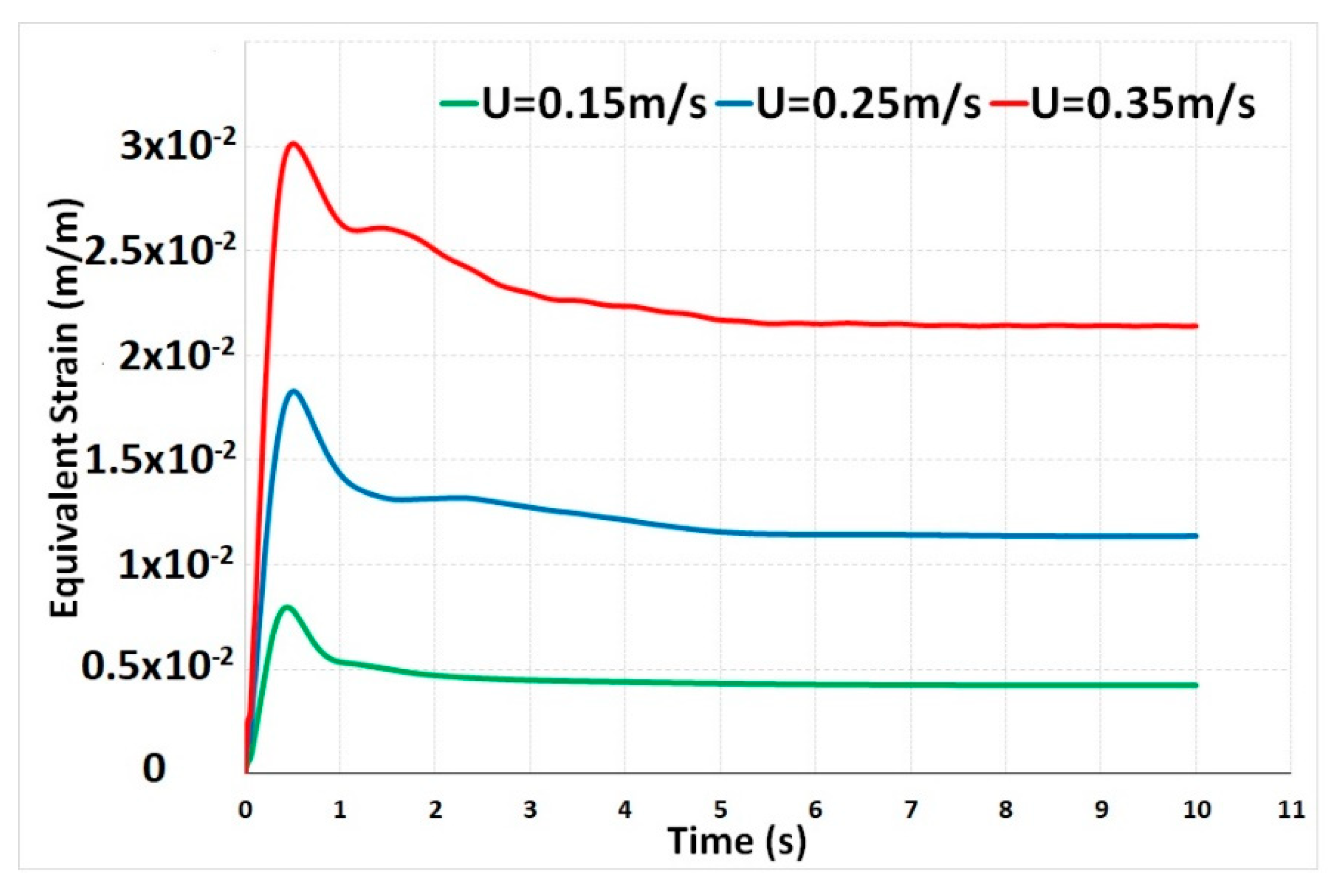
3.1. Comparison between Experimental and Numerical Results

High-speed camera (HSC) measurements were carried out for the three-dimensional flexible beam model at one Reynolds number (42,500). The close-circuit water channel could supply 0.25 m/s as the highest velocity, so the highest Reynolds number for flexible beam was 42,500 in this experiment work. The numerical simulation was done at the same conditions, as used for the experiment. The results of numerical and experimental data were compared regarding the total deformation, Figure 8. The total deformation shape in the numerical model agrees well with the deformation obtained from HSC measurements for a Reynolds number of 42,500. A point (red point) was selected at the top of the T-shaped flexible beam for the tracking maximum displacement of the T-shaped flexible beam. When the T-shaped flexible beam has a vertical position, the red point is at position 1. After deformation, the red point changes from position 1 to position 2. The maximum displacement is the distance between position 1 and position 2.

Table 4. Comparison of maximum deformation of T-shaped flexible beam for Re = 42,500, t = 6 s, and t = 10 s.

Re = 42,500	t = 6 s (Figure 8a–c)	t = 10 s (Figure 8d–f)
Experimental model deformation (m)	0.0205 ± 0.001	0.0202 ± 0.001
Numerical model deformation (m)	0.0193	0.0191

shows the maximum deformation of the T-shaped flexible beam at t = 6 s and t = 10 s for numerical and experimental models.

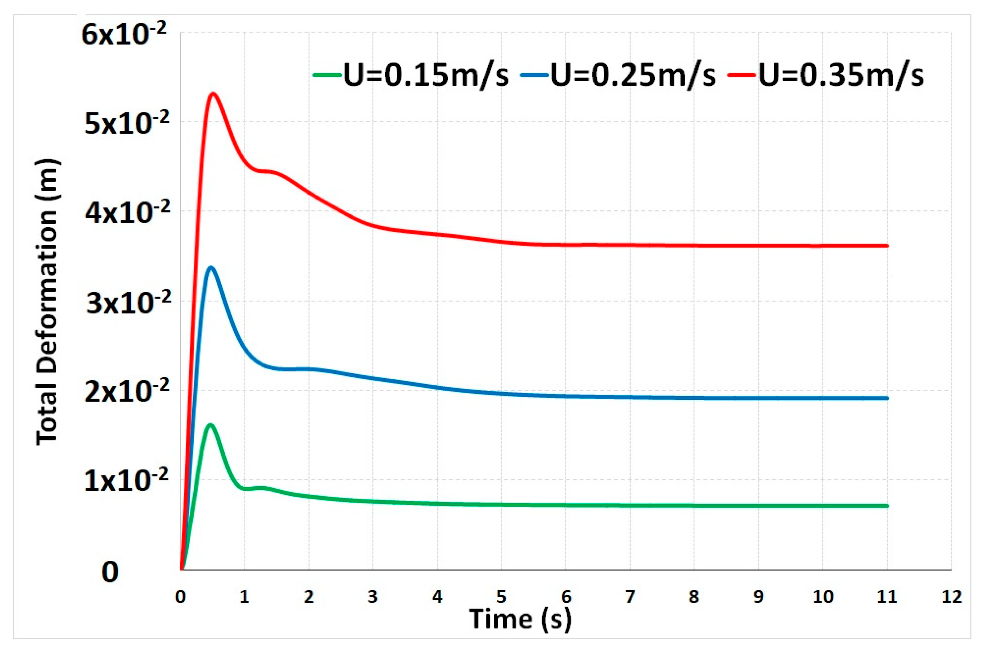
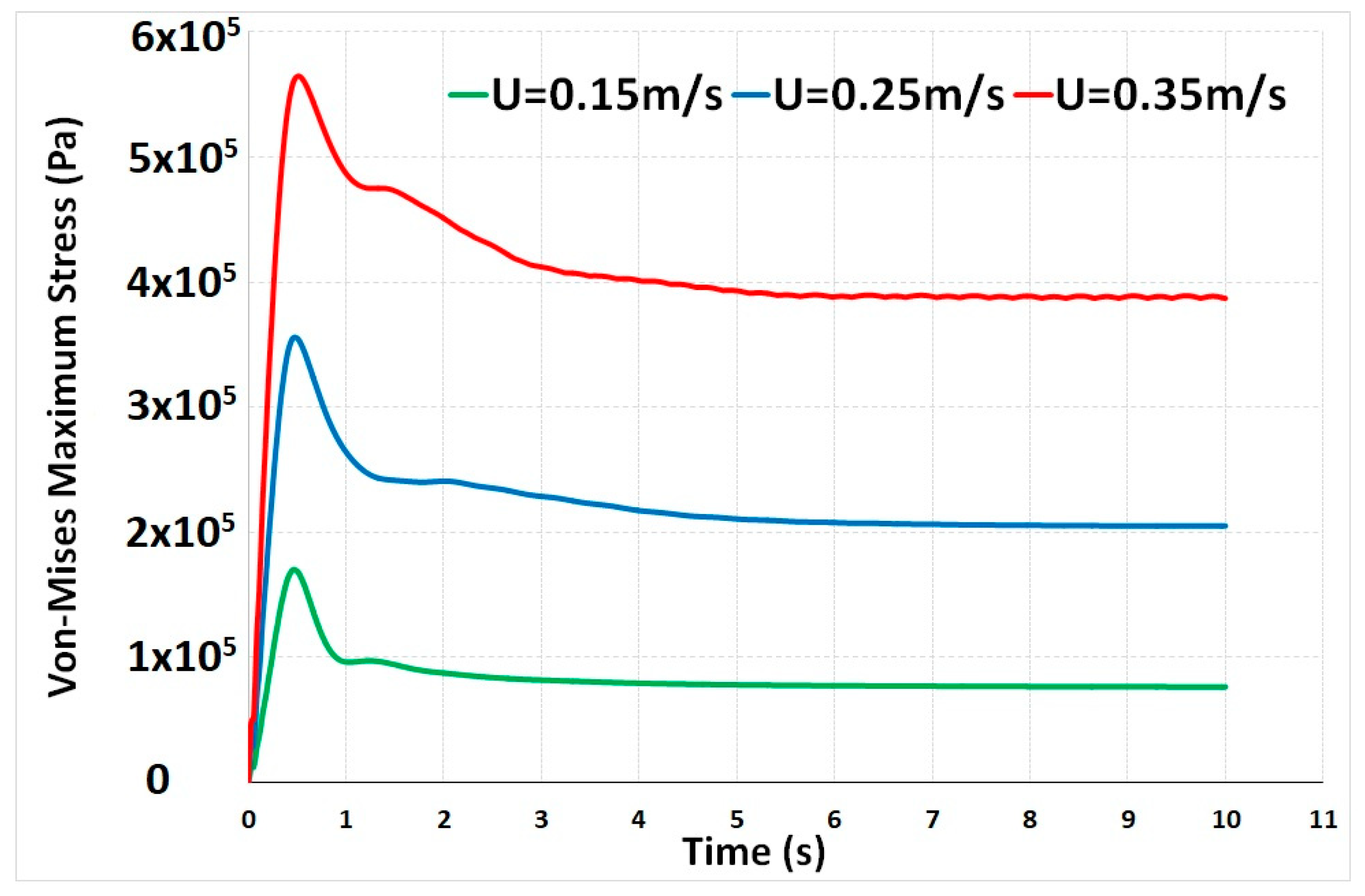
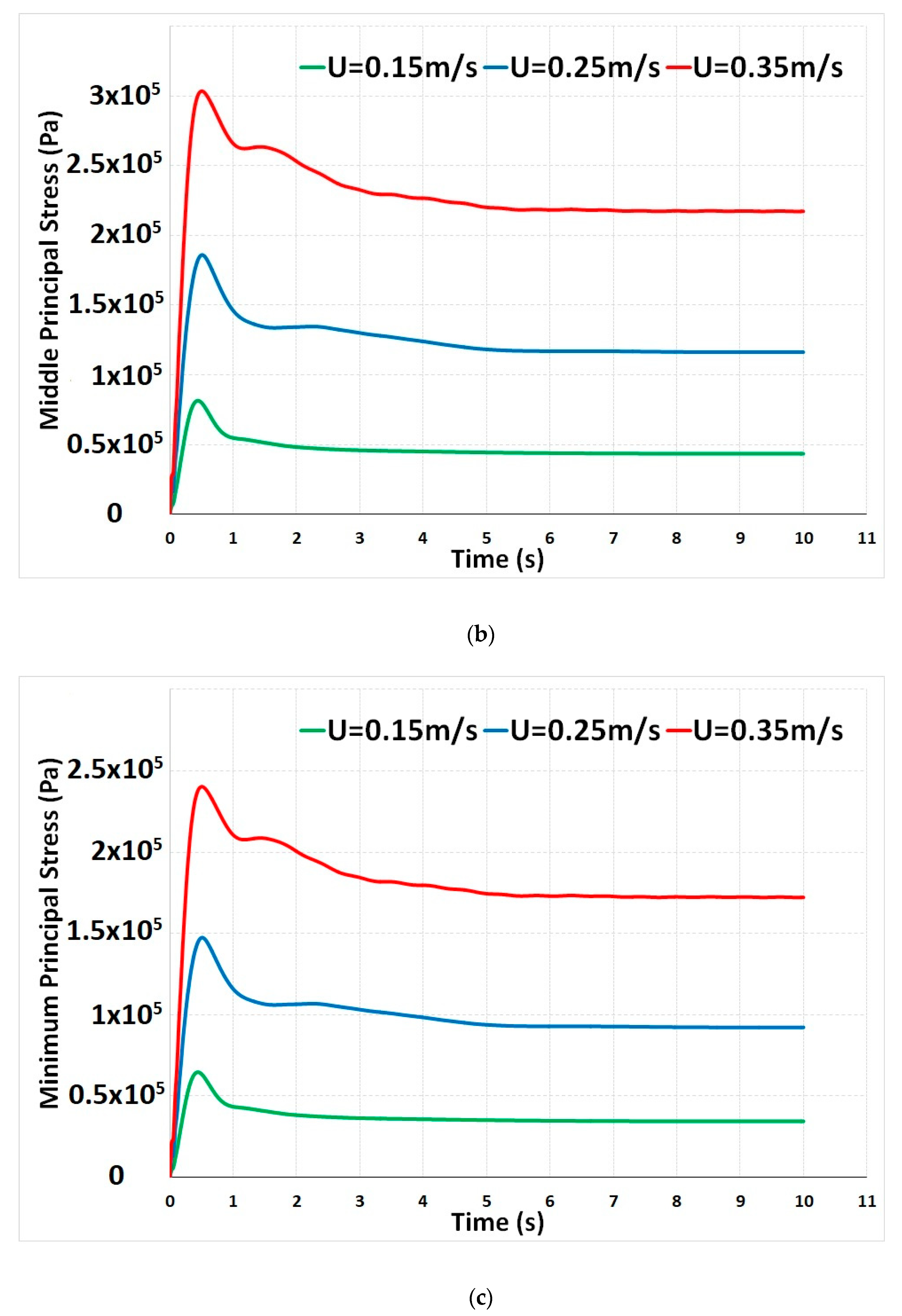
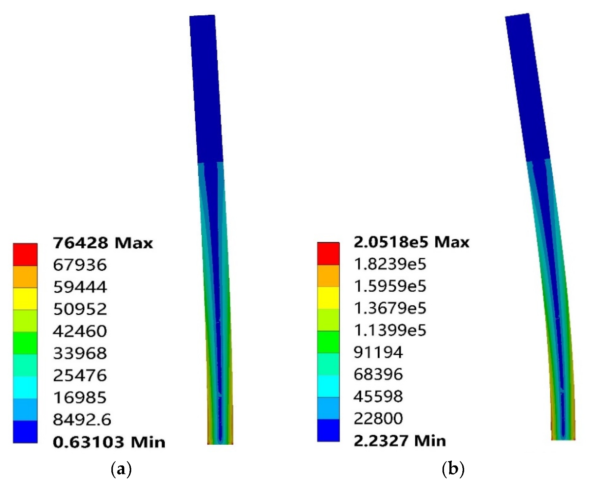
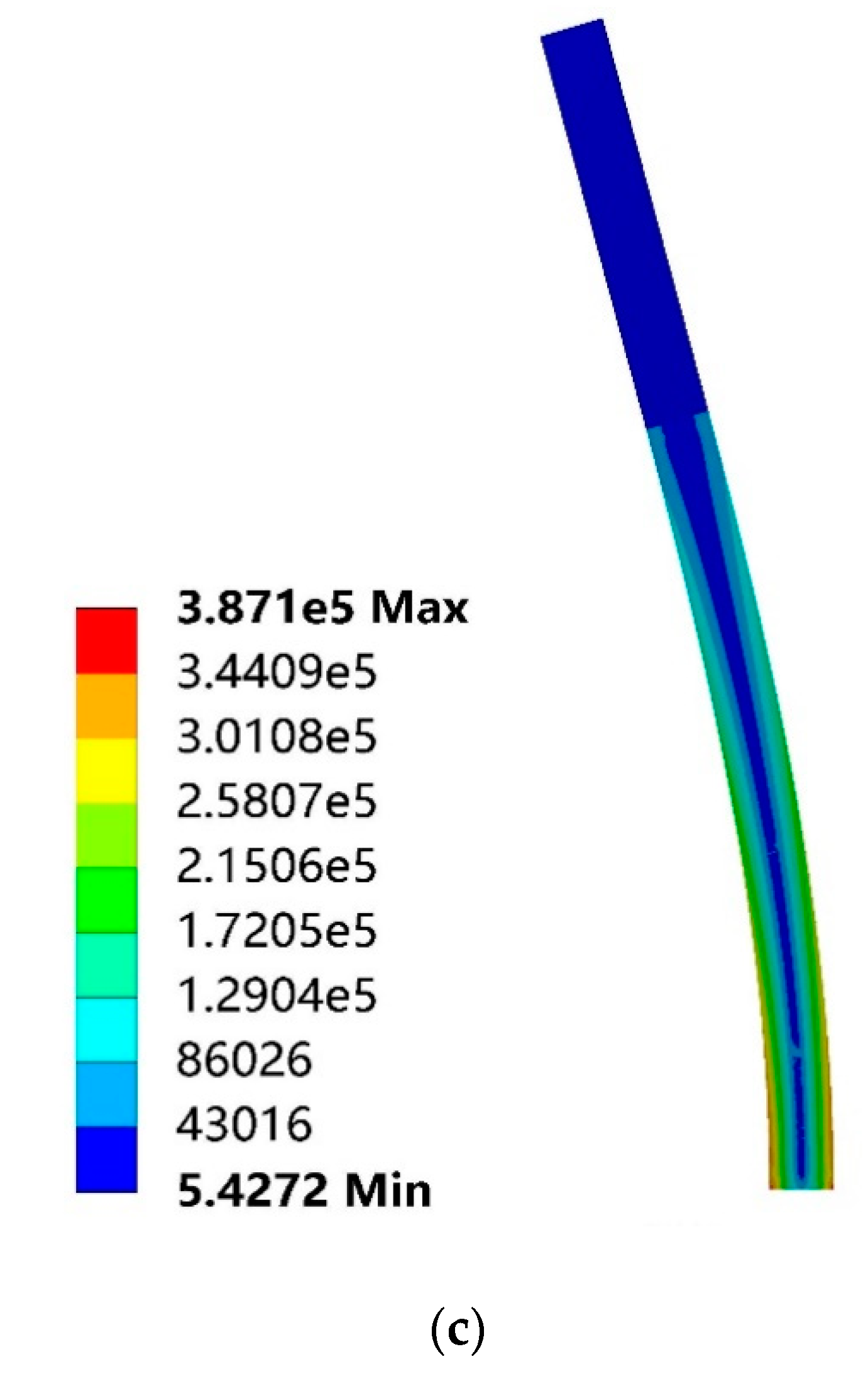
3.2. Deformation and Stress Study

The T-shaped flexible beam was validated at a Reynolds number of 42,500 (U = 0.25 m/s), and then, it was investigated at two different Reynolds numbers of 25,500 (U = 0.15 m/s) and 59,500 (U = 0.35 m/s). Totally, The T-shaped flexible beam was studied in three various Reynolds numbers numerically. Total deformation was calculated numerically in this study. Total deformation can be computed by using Equation (13)

$$\mathrm{U}=\sqrt{{\mathrm{U}}_{\mathrm{x}}^2+{\mathrm{U}}_{\mathrm{y}}^2+{\mathrm{U}}_{\mathrm{z}}^2}$$

(13)

where ${\mathrm{U}}_{\mathrm{x}}$ is component deformation in the x direction, ${\mathrm{U}}_{\mathrm{y}}$ is component deformation in the y direction, ${\mathrm{U}}_{\mathrm{z}}$ is component deformation in the z direction. Figure 9 shows total deformation record from t = 0 s to t = 10 s at three different velocities of 0.15, 0.25, and 0.35 m/s. In all velocities, deformation of the T-shaped flexible beam increased in time, then it started to decrease and, finally, it had a constant value. The deformation of the T-shaped flexible beam increased with increasing velocity. The outer load also changed with velocity. The T-shaped flexible beam bent more and more when velocity increases. It seems that the maximum value of deformation happens early for minimum velocity. We can observe that the maximum value of deformation occurs at t = 0.47 s when velocity is U = 0.15 m/s, and also, it occurs at t = 0.511 s when velocity is U = 0.35 m/s. Maximum stress (Von Mises stress) of the T-shaped flexible beam happened at maximum inlet velocity between three different inlet velocities.

Von Mises stress was calculated numerically in this study. Von Mises stress can be calculated by using Equation (14)

$${\mathsf{\sigma }}_{\mathrm{e}}={\left[\frac{{\left({\mathsf{\sigma }}_1-{\mathsf{\sigma }}_2\right)}^2+{\left({\mathsf{\sigma }}_2-{\mathsf{\sigma }}_3\right)}^2+{\left({\mathsf{\sigma }}_3-{\mathsf{\sigma }}_1\right)}^2}{2}\right]}^{1/2}$$

(14)

where ${\mathsf{\sigma }}_1$ stress statestress in the x direction, ${\mathsf{\sigma }}_2$ is stress statestress in the y direction, and ${\mathsf{\sigma }}_3$ is stress statestress in the z direction. The maximum stress and maximum deformation of the beam have similar behavior, so we can figure out that stress changes like deformation in all velocities. Figure 10 shows maximum stress of beam that changes by time, and it occurs obviously on the bottom of the beam. Figure 11a–c show maximum principal stress, middle principal stress, and minimum principal stress of beam that changes by time.

Equivalent strain was computed numerically in this study. Equivalent strain can be calculated by using Equation (15)

$${\mathsf{\epsilon }}_{\mathrm{e}}=\frac{1}{1+{\mathsf{\upsilon }}^{\prime }}{\left(\frac{1}{2}\left[{\left({\mathsf{\epsilon }}_1-{\mathsf{\epsilon }}_2\right)}^2+{\left({\mathsf{\epsilon }}_2-{\mathsf{\epsilon }}_3\right)}^2+{\left({\mathsf{\epsilon }}_3-{\mathsf{\epsilon }}_1\right)}^2\right]\right)}^{\frac{1}{2}}$$

(15)

where ${\mathsf{\epsilon }}_1$ is principal strain in the x direction, ${\mathsf{\epsilon }}_2$ is principal strain in the y direction, ${\mathsf{\epsilon }}_3$ is principal strain in the z direction, and ${\upsilon }^{\prime }$ is effective Poisson’s ratio. Figure 12 shows equivalent strain of beam that changes by time.

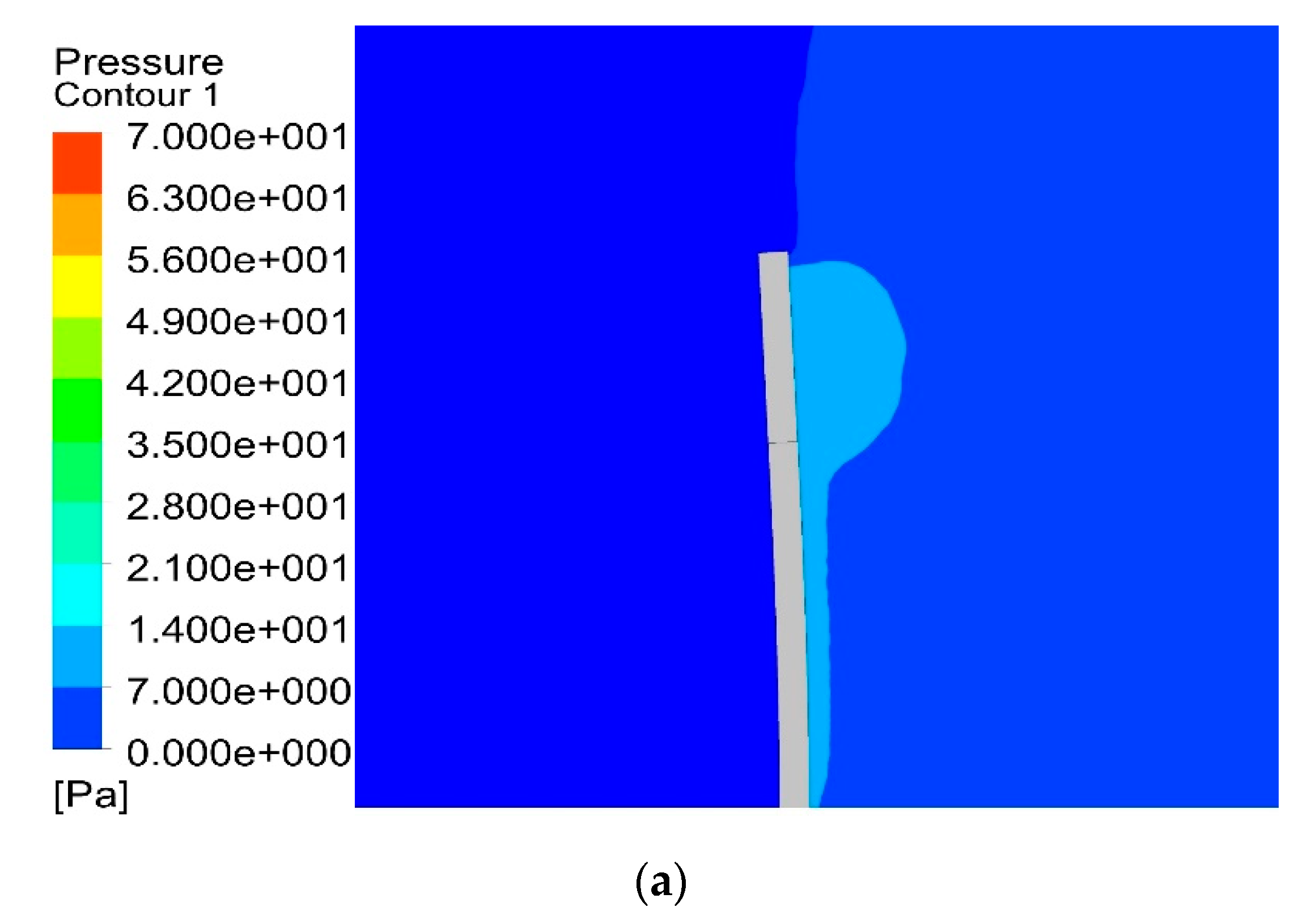
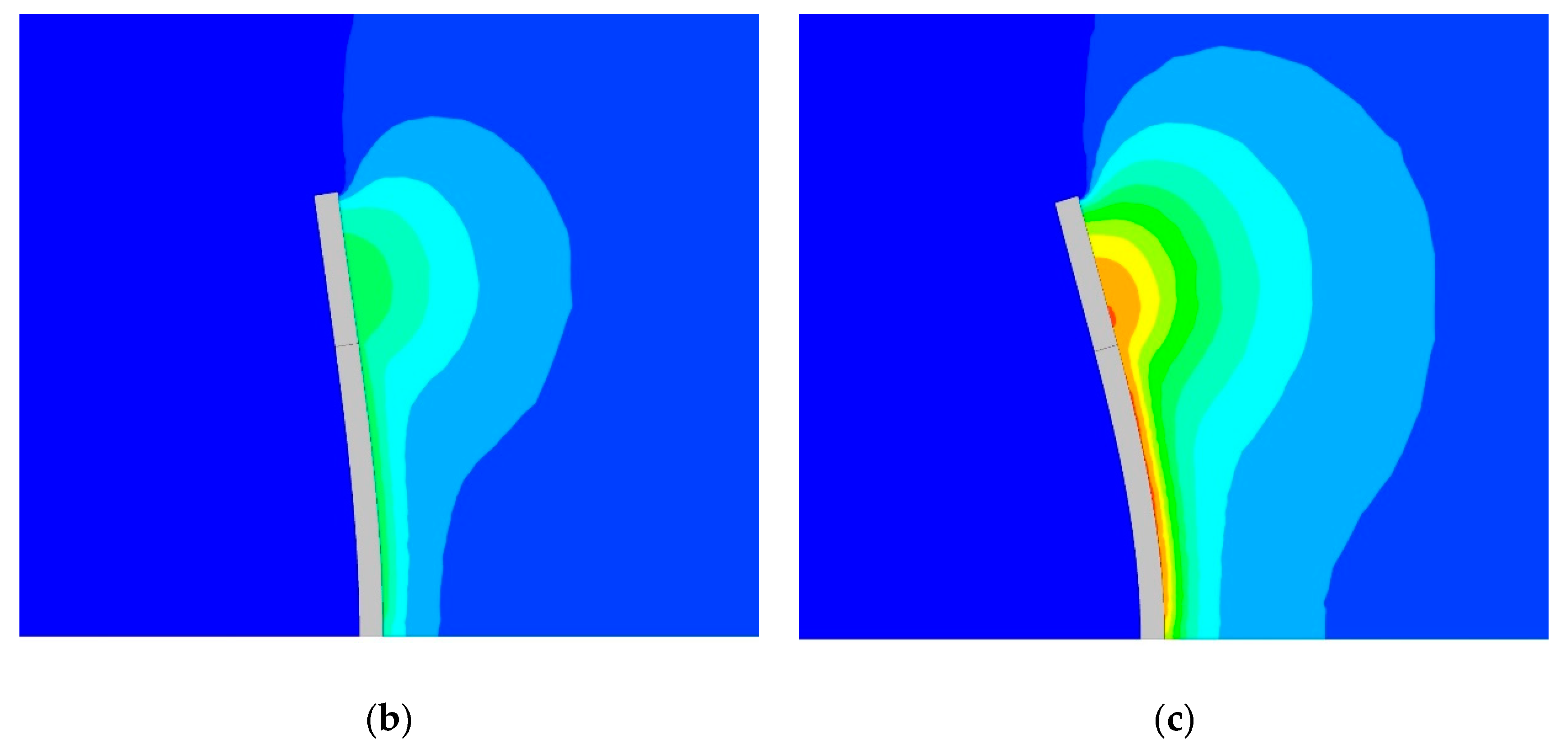
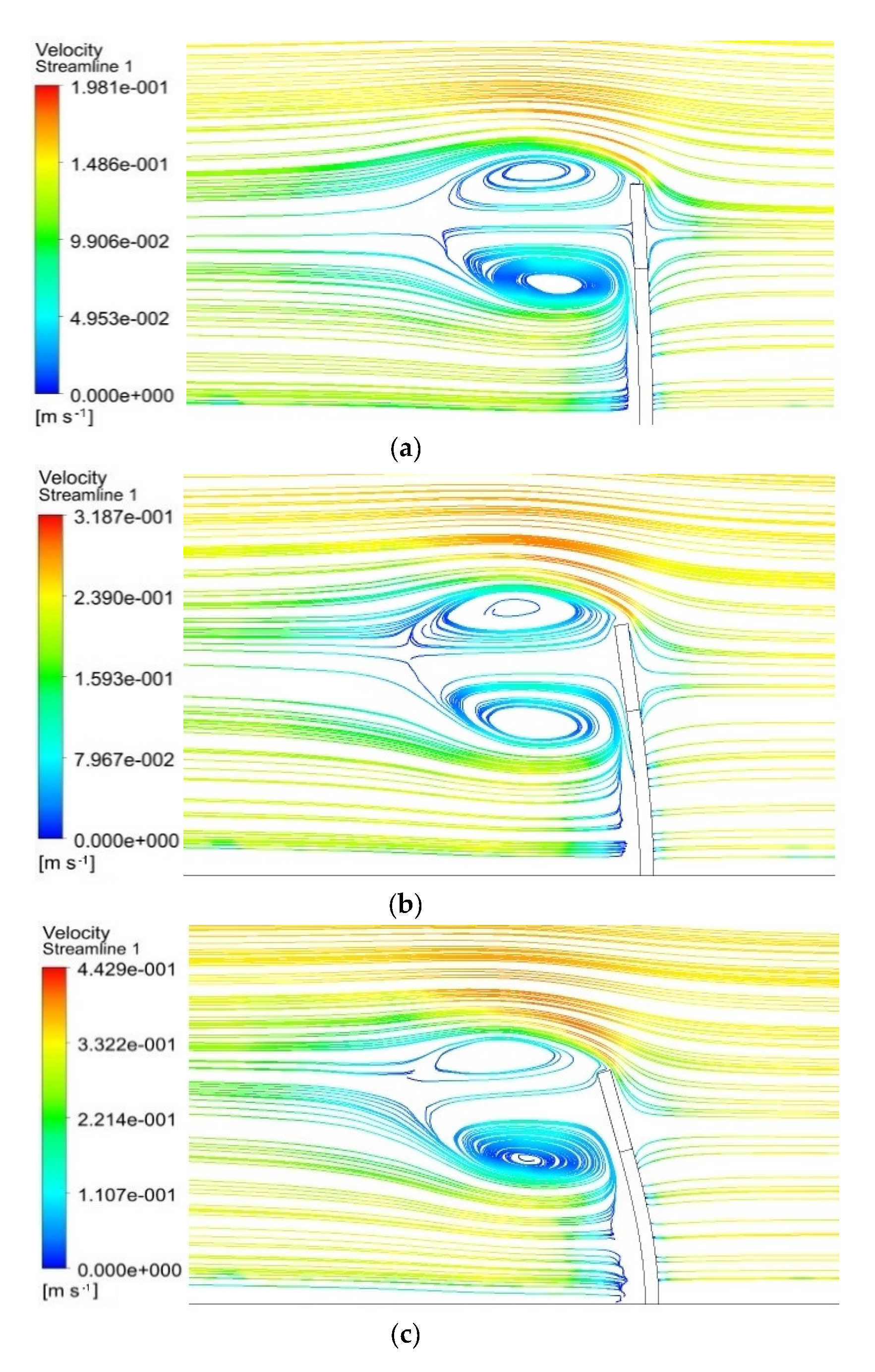
3.3. Contours Plots of Numerical Study

Deformation of the T-shaped flexible beam was shown for three different Reynolds numbers of 25,500 (U = 0.15 m/s), 42,500 (U = 0.25 m/s), and 59,500 (U = 0.35 m/s) at t = 10 s, Figure 13. The stress of the T-shaped flexible beam was illustrated for three different Reynolds numbers of 25,500, 42,500, and 59,500 at t = 10 s, Figure 14. It was realized that maximum deformation and stress occurred at the maximum Reynolds number, because the T-shaped flexible beam has a large pressure in the front surface.

Pressure contours at the solution domain were plotted in Figure 15 for t = 10 s. When flow around a T-shaped flexible beam was studied, there was a large pressure on the front surface of T-shaped flexible beams. Figure 16 also showed lower pressure regions at the top region of the T-shaped flexible beam implying flow separation. It was noted that the pressure difference between the front and back surface of T-shaped flexible beams was large. In addition to pressure contours, streamline contours were plotted in Figure 16 for t = 10 s. It was revealed that recirculation regions were formed behind the T-shaped flexible beams. Recirculation regions were near the top region of the T-shaped flexible beam, because the separation happened near the head of the T-shaped flexible beam.

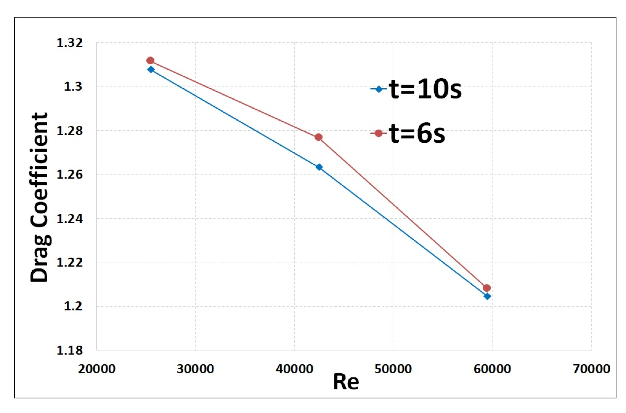
3.4. Drag Coefficients Study

When the body locates in fluid flow, it can experience a certain amount of drag force (Olcay et al. [28], Batchelor [32], and Vasudev et al. [33]). Drag force was given by

$$F_D=F_{D\_pressure}+F_{D\_viscous}=\oint P\widehat{n}.{\widehat{e}}_{d}dS+\oint {\tau }_w\widehat{t}.{\widehat{e}}_{d}dS$$

(16)

where $F_{D\_pressure}$ and $F_{D\_viscous}$ are drag forces in the x-direction due to the pressure and viscous effects. Here, $p$ is the pressure on the T-shaped flexible beam, and ${\tau }_w$ is the wall shear stress on the surface of T-shaped flexible beam.

Drag force studies are shown in

Table 5. Change in drag force with the Reynolds numbers for t = 6 s and t = 10 s.

Reynolds Umbers	Drag Force, t = 6 s	Drag Force, t = 10 s
25,500 (U = 0.15 m/s)	0.09591	0.09563
42,500 (U = 0.25 m/s)	0.25932	0.25663
59,500 (U = 0.35 m/s)	0.48103	0.47961

for t = 6 s and t = 10 s. It was noted that the drag force increased with increased Reynolds numbers for T-shaped flexible beam.

Once the drag force was obtained, the drag coefficient was studied using Equation (9).

$$C_d=\frac{F_{Drag}}{\frac{1}{2}\rho U^{2}A}$$

(17)

where $C_d$ is drag coefficient, $F_{Drag}$ is Drag force, $\rho$ is density of the fluid, $U$ is velocity of fluid, and $A$ is the reference area (the frontal area of the body). Drag coefficient was plotted in Figure 17. It was also realized that the drag coefficient decreased with increased Reynolds numbers for T-shaped flexible beam.

4. Conclusions

In this study, the deformation of a T-shaped flexible beam was investigated at 0.25 m/s inlet velocity. A three-dimensional T-shaped flexible beam was placed into a close-circuit water channel for high-speed camera system (HSC) measurements. The results of a three-dimensional T-shaped flexible beam agreed well with the results of HSC measurements for 0.25 m/s inlet velocity. Then, two additional inlet velocities were noticed for a flexible beam, and those velocities were examined for the T-shaped flexible beam. A two-way FSI coupling method was employed for solving fluid and solid parts. The dynamic mesh method was used for grid, and mesh was updated in every time step in fluid and solid sides. Deformation, maximum stress, and minimum stress of the T-shaped flexible beam were calculated, and also, velocity distribution and pressure distribution of the flow around the T-shaped flexible beam were computed at various velocities in the numerical model. The results reveal that deformation and stress in the flexible beam has increased with increasing velocity. It was also found that a large pressure region was created on the front surface of the T-shaped flexible beam and flow separation happened in the head of the T-shaped flexible beam. It was concluded that high velocity caused the drag force to be larger when compared with low velocity, so high drag force caused a large deformation and high stress in the T-shaped flexible beam. We carried out a validation study. The results of experimental and numerical methods were compared in the present study. In this study, the percent error of maximum deformation between experimental and numerical methods is nearly 4%~5%. The study also revealed that the system coupling method can be used in fluid–structure interaction applications and a two-way FSI coupling method has high efficiency, so this method can be employed in various engineering fields such as mechanical, civil, and ocean engineering.

References

1. Chimakurthi, S.K.; Reuss, S.; Tooley, M.; Scampoli, S. ANSYS workbench system coupling: A state-of-the-art computational framework for analyzing multiphysics problems. Eng. Comput. 2017, 34, 385–411. [Google Scholar] [CrossRef]
2. Gluck, M.; Breuer, M.; Durst, F.; Halfmann, A.; Rank, E. Computation of fluid–structure interaction on lightweight structures. J. Wind Eng. Ind. Aerodyn. 2001, 89, 1351–1368. [Google Scholar] [CrossRef]
3. Dhavalikar, S.; Awasare, S.; Joga, R.; Kar, A.R. Whipping response analysis by one way fluid structure interaction—A case study. Ocean Eng. 2015, 103, 10–20. [Google Scholar] [CrossRef]
4. Narayanan, K.V.; Vengadesan, S.; Murali, K. Wall proximity effects on the flow past cylinder with flexible filaments. Ocean Eng. 2018, 157, 54–61. [Google Scholar] [CrossRef]
5. Hassani, M.; Mureithi, N.W.; Gosselin, F.P. Large coupled bending and torsional deformation of an elastic rod subjected to fluid flow. J. Fluids Struct. 2016, 62, 367–383. [Google Scholar] [CrossRef]
6. Juan, J.S.; Carrillo, G.V.; Tinoco, R.O. Experimental observations of 3D flow alterations by vegetation under oscillatory flows. Environ. Fluid Mech. 2019, 19, 1497–1525. [Google Scholar] [CrossRef]
7. Mantecon, J.G.; Neto, M.M. Numerical methodology for fluid-structure interaction analysis of nuclear fuel plates under axial flow conditions. Nucl. Eng. Des. 2018, 333, 76–86. [Google Scholar] [CrossRef]
8. Ghelardi, S.; Freda, A.; Rizzo, C.M.; Villa, D. A fluid structure interaction case study on a square sail in a wind tunnel. Ocean Eng. 2018, 163, 136–147. [Google Scholar] [CrossRef]
9. Liu, Z.G.; Liu, Y.; Lu, J. Fluid-structure interaction of single cylinder in axial flow. Comput. Fluids 2012, 56, 143–151. [Google Scholar] [CrossRef]
10. Xu, L.; Tian, F.-B.; Young, J.; Lai, J.C.S. A novel geometry-adaptive Cartesian grid based immersed boundary–lattice Boltzmann method for fluid–structure interactions at moderate and high Reynolds numbers. J. Comput. Phys. 2018, 375, 22–56. [Google Scholar] [CrossRef]
11. Wang, C.; Sun, M.; Shankar, S.; Xing, S.; Zhang, L. CFD Simulation of Vortex Induced Vibration for FRP composite riser with different modeling methods. Appl. Sci. 2018, 8, 684. [Google Scholar] [CrossRef] [Green Version]
12. Dong, D.; Chen, W.; Shi, S. Coupling motion and energy harvesting of two side-by-side flexible plates in a 3D uniform flow. Appl. Sci. 2016, 6, 141. [Google Scholar] [CrossRef] [Green Version]
13. Wang, L.; Currao, G.M.D.; Han, F.; Neely, A.J.; Young, J.; Tian, F.B. An immersed boundary method for fluid–structure interaction with compressible multiphase flows. J. Comput. Phys. 2017, 346, 131–151. [Google Scholar] [CrossRef] [Green Version]
14. Turek, S.; Hron, J. Proposal for numerical benchmarking of fluid-structure interaction between an elastic object and laminar incompressible flow. Fluid Struct. Interact. 2006, 53, 371–385. [Google Scholar]
15. Wang, H.; Zhai, Q.; Zhang, J. Numerical study of flow-induced vibration of a flexible plate behind a circular cylinder. Ocean Eng. 2018, 163, 419–430. [Google Scholar] [CrossRef]
16. Zheng, X.; Xue, Q.; Mittal, R.; Beilamowicz, S. A coupled sharp-interface immersed boundary-finite-element method for flow-structure interaction with application to human phonation. J. Biomech. Eng. 2010, 132. [Google Scholar] [CrossRef] [Green Version]
17. Wang, M.; Avital, E.J.; Bai, X.; Ji, C.; Xu, D.; Williams, J.J.; Munjiza, A. Fluid–structure interaction of flexible submerged vegetation stems and kinetic turbine blades. Comput. Part. Mech. 2019. [Google Scholar] [CrossRef] [Green Version]
18. Mittal, R.; Dong, H.; Bozkurttas, M.; Najjar, F.M.; Vargas, A.; Von Loebbecke, A. A versatile sharp interface immersed boundary method for incompressible flows with complex boundaries. J. Comput. Phys. 2008, 227, 4825–4852. [Google Scholar] [CrossRef] [Green Version]
19. Nestola, M.G.C.; Becsek, B.; Zolfaghari, H.; Zulian, P.; Marinis, D.D.; Krause, R.; Obrist, D. An immersed boundary method for fluid-structure interaction based on variational transfer. J. Comput. Phys. 2019, 398, 108884. [Google Scholar] [CrossRef]
20. Peskin, C.S. The immersed boundary method. Acta Numer. 2002, 11, 479–517. [Google Scholar] [CrossRef] [Green Version]
21. Hron, J.; Turek, J. A monolithic FEM/multigrid solver for an ALE formulation of fluid-structure interaction with applications in biomechanics. Fluid Struct. Interact. 2006, 146–170. [Google Scholar] [CrossRef]
22. Griffith, B.E.; Luo, X. Hybrid finite difference/finite element immersed boundary method. Int. J. Numer. Methods Biomed. Eng. 2017, 33. [Google Scholar] [CrossRef] [PubMed] [Green Version]
23. Nassiri, A.; Chini, G.; Vivek, A.; Daehn, G.; Kinsey, B. Arbitrary Lagrangian–Eulerian finite element simulation and experimental investigation of wavy interfacial morphology during high velocity impact welding. Mater. Des. 2015, 88, 345–358. [Google Scholar] [CrossRef]
24. Tabatabaei-Malazi, M.; Okbaz, A.; Olcay, A.B. Numerical investigation of a longfin inshore squid’s flow characteristics. Ocean Eng. 2015, 108, 462–470. [Google Scholar] [CrossRef]
25. Olcay, A.B.; Tabatabaei-Malazi, M.; Okbaz, A.; Heperkan, H.A.; Firat, E.; Ozbolat, V.; Gokcen, M.G.; Sahin, B. Experimental and numerical investigation of a longfin inshore squid’s flow characteristics. J. Appl. Fluid Mech. 2017, 10, 21–30. [Google Scholar] [CrossRef]
26. Eren, E.T.; Tabatabaei-Malazi, M.; Temir, G. Numerical investigation on the collision between a solitary wave and a moving cylinder. Water 2020, 12, 2167. [Google Scholar] [CrossRef]
27. Howse, J. OpenCV Computer Vision with Python; Packt Publishing Ltd.: Birmingham, UK, 2013. [Google Scholar]
28. Olcay, A.B.; Tabatabaei-Malazi, M. The effects of a longfin inshore squid’s fins on propulsive efficiency during underwater swimming. Ocean Eng. 2016, 128, 173–182. [Google Scholar] [CrossRef]
29. ANSYS Fluent Theory Guide; ANSYS, Inc.: Canonsburg, PA, USA, 2016; pp. 39–136.
30. Bathe, K.J. Finite Element Procedures; Prentice-Hall: Englewood Cliffs, NJ, USA, 1996. [Google Scholar]
31. Chung, J.; Hulbert, G.M. A time integration algorithm for structure dynamic with improved numerical dissipation: The generalized-α method. J. Appl. Mech. 1993, 60, 371. [Google Scholar] [CrossRef]
32. Batchelor, G.K. An Introduction to Fluid Dynamics; Cambridge University Press: Cambridge, UK, 2000. [Google Scholar]
33. Vasudev, K.L.; Sharma, R.; Bhattacharyya, S.K. A multi-objective optimization design framework integrated with CFD for the design of AUVs. Methods Oceanogr. 2014, 10, 138–165. [Google Scholar] [CrossRef]
Figure 1. Schematics showing the dimensions of the beam.
Jmse 08 00714 g001
Figure 2. Schematics of the experiment setup: (a) experimental arrangement in the recirculating water flume; (b) high-speed camera on one side of the flume; (c) and (d) side views.
Jmse 08 00714 g002aJmse 08 00714 g002b
Figure 3. Standardization test.
Jmse 08 00714 g003
Figure 4. Flow chart of image processing program.
Jmse 08 00714 g004
Figure 5. Numerical steps of system coupling.
Jmse 08 00714 g005
Figure 6. Details of the computational domain and boundary conditions.
Jmse 08 00714 g006
Figure 7. (a) Computational mesh of fluid domain, (b) enlarged view around beam surface, and (c) computational mesh of beam.
Jmse 08 00714 g007
Figure 8. Comparison of total deformation of T-shaped flexible beam for Re = 42,500 and t = 6 s. (a) Experiment (high-speed camera system (HSC)), (b) experiment (HSC) with image track program, and (c) numerical (CFD). Comparison of total deformation of T-shaped flexible beam for Re = 42,500 and t = 10 s. (d) Experiment (HSC), (e) experiment (HSC) with image track program, and (f) numerical (CFD).
Jmse 08 00714 g008
Figure 9. Variation of total deformation of T-shaped flexible beam between t = 0 s and 10 s.
Jmse 08 00714 g009
Figure 10. Variation of Von Mises maximum stress of T-shaped flexible beam between t = 0 s and 10 s.
Jmse 08 00714 g010
Figure 11. (a) Variation of maximum principal stress of T-shaped flexible beam between t = 0 s and 10 s. (b) Variation of middle principal stress of T-shaped flexible beam between t = 0 s and 10 s. (c) Variation of minimum principal stress of T-shaped flexible beam between t = 0 s and 10 s.
Jmse 08 00714 g011aJmse 08 00714 g011b
Figure 12. Variation of equivalent strain of T-shaped flexible beam between t = 0 s and 10 s.
Jmse 08 00714 g012
Figure 13. Deformation (m) of T-shaped flexible beam at t = 10 s (a) Re = 25,500, (b) Re = 42,500, and (c) Re = 59,500.
Jmse 08 00714 g013aJmse 08 00714 g013b
Figure 14. Stress (Pa) of T-shaped flexible beam at t = 10 s (a) Re = 25,500, (b) Re = 42,500, and (c) Re = 59,500.
Jmse 08 00714 g014aJmse 08 00714 g014b
Figure 15. Pressure distribution (Pa) of T-shaped flexible beam at t = 10 s (a) Re = 25,500, (b) Re = 42,500, and (c) Re = 59,500.
Jmse 08 00714 g015aJmse 08 00714 g015b
Figure 16. Streamline (m) of T-shaped flexible beam at t = 10 s (a) Re = 25,500, (b) Re = 42,500, and (c) Re = 59,500.
Jmse 08 00714 g016
Figure 17. Change in drag coefficient with Reynolds numbers for (a) t = 6 s and (b) t = 10 s.
Jmse 08 00714 g017