Article

Key Environmental Factors Controlling Planktonic Foraminiferal and Pteropod Community’s Response to Late Quaternary Hydroclimate Changes in the South Aegean Sea (Eastern Mediterranean)

by
Christina Giamali
1,2,*,
George Kontakiotis
1,*,
Efterpi Koskeridou
1,
Chryssanthi Ioakim
3 and
Assimina Antonarakou
1
1
Department of Historical Geology and Paleontology, Faculty of Geology and Geoenvironment, National and Kapodistrian University of Athens, Panepistimiopolis, 15784 Athens, Greece
2
The Goulandris Natural History Museum, Levidou 13, 14562 Kifissia, Greece
3
Institute of Geology and Mineral Exploration (I.G.M.E.), Olympic Village, 13677 Acharnae, Greece
*
Authors to whom correspondence should be addressed.
J. Mar. Sci. Eng. 2020, 8(9), 709; https://doi.org/10.3390/jmse8090709
Submission received: 27 August 2020 / Revised: 9 September 2020 / Accepted: 10 September 2020 / Published: 14 September 2020
(This article belongs to the Special Issue Climate Change and Marine Geological Dynamics)

Abstract

:
A multidisciplinary study was conducted in order to investigate the environmental factors affecting the planktonic foraminiferal and pteropod communities of the south Aegean Sea. Aspects of the Late Quaternary paleoceanographic evolution were revealed by means of quantitative analyses of planktonic foraminiferal and pteropod assemblages (including multivariate statistical approach; principal component analysis (PCA)), the oxygen (δ18O) and carbon (δ13C) isotopic composition of planktonic foraminifera and related paleoceanographic (planktonic paleoclimatic curve (PPC), productivity (E-index), stratification (S-index), seasonality) indices, extracted by the gravity core KIM-2A derived from the submarine area between Kimolos and Sifnos islands. Focusing on the last ~21 calibrated thousands of years before present (ka BP), cold and eutrophicated conditions were identified during the Late Glacial period (21.1–15.7 ka BP) and were followed by warmer and wetter conditions during the deglaciation phase. The beginning of the Holocene was marked by a climatic amelioration and increased seasonality. The more pronounced environmental changes were identified during the deposition of the sapropel sublayers S1a (9.4–7.7 ka BP) and S1b (6.9–6.4 ka BP), with extremely warm and stratified conditions. Pteropod fauna during the sapropel deposition were recorded for the first time in the south Aegean Sea, suggesting arid conditions towards the end of S1a. Besides sea surface temperature (SST), which shows the highest explanatory power for the distribution of the analyzed fauna, water column stratification, primary productivity, and seasonality also control their communities during the Late Quaternary.

1. Introduction

The Aegean Sea is an ideal archive to investigate climatic evolution at both global and local scale because of its intermediate position between the higher- and lower-latitude climate systems [1,2,3], high sedimentation rate marine records compared to the open Mediterranean Sea [4,5,6,7], and its paleo-latitudinal and land-locked configuration [8,9]. Such marginal seas are often more responsive to paleoceanographic and paleoclimatic changes than global oceans, with climatic signals to be recorded in an amplified fashion in Mediterranean properties such as temperature, salinity and specific elemental concentrations, because of their smaller size and partial isolation [10], and therefore can be considered miniature oceans. In addition to interactions with the Black Sea, northern Aegean, and Levantine basins with remote and local atmospheric forcing [1,11], the south Aegean Sea is characterized by intense biogeochemical contrasts in its hydrology in response to a climatic gradient from mid-latitude to subtropical regimes that appears to be very sensitive to climate changes. However, most of the current paleoclimatic and paleoceanographic studies are still limited to deep marine records [6,12,13,14,15], and consequently little is known about the continental shelf and/or coastal areas within this marginal Sea [16,17,18,19,20,21].
Environmental changes related to the different water column and/or sediment characteristics can be recorded virtually instantaneously in paleoceanographic proxy data, such as stable isotope and other geochemical ratios [22,23,24,25,26,27,28,29,30,31], and micro-fossil abundances, such as planktonic foraminifera and pteropods [15,17,28,32,33,34,35,36]. This makes them extremely valuable for both stratigraphic correlations and paleoenvironmental/paleoclimate reconstructions [15,23,28,29,32,35,37,38,39,40,41,42,43,44,45]. Their significance in the study of modern and past marine ecosystems in the eastern Mediterranean Sea is well underlined [20,31,46,47,48,49,50,51]. Particularly, they are used as indicators of temperature, salinity, density, and nutrient content of the water column, making it possible to identify past circulation through the sedimentary record [7,15,29,47,52,53] and detect long- and short-term paleoclimatic and paleoceanographic changes in the study area [6,10,12,15,16,53,54,55] during the last glacial cycle.
Pteropods are widespread and abundant in the global ocean and entirely adapted to a pelagic life cycle [56,57]. Owing to the aragonite nature of their shells which increases their weight as settling particles and hence their sinking speed [58], their deposition is expected to be close to their habitat [59]. Particularly in the Mediterranean Sea, preservation of pteropods shells is excellent as a result of the relatively shallow water, high bottom water temperatures, and probably the limited number of mud feeders [60]. A considerable number of studies (e.g., [33,34,61,62,63,64,65,66]) have shown that Late Quaternary pteropod assemblages and their distribution pattern in the world oceans have changed with temperature and the overall climatic conditions that also affect the aragonite compensation depth (ACD). Recent studies [67] have shown that modern eastern Mediterranean pteropod communities are found to be more abundant than in those at western Mediterranean Sea. Their abundances are positively correlated with the aragonite saturation state (Ωar), O2 concentration, pH, salinity and temperature, and negatively correlated with nutrient concentrations [67,68]. However, pteropod assemblages and their distribution in the Aegean Sea during the Late Quaternary are poorly documented.
The present study focuses on identifying and describing key environmental factors that control Late Quaternary planktonic foraminiferal and pteropod distribution in the south Aegean Sea, based on marine sediments retrieved by a 2-m long gravity (KIM-2A) core. In addition, paleoclimatic data were revealed from their distribution patterns coupled with variations of oxygen and carbon isotopic signals. The combination of the above data enables speculation on the factors’ response to the climatic changes.

2. Regional and Climatic Setting

The Aegean Sea is in the northern sector of the eastern Mediterranean (Figure 1a), between the Turkish coastline to the east, the Greek mainland to the north and west, and bounded on the south by the island of Crete and Cretan Arc. It is connected to the Black Sea through the Straits of Bosporus and Dardanelles, and to the Levantine Sea through several larger and deeper straits between Peloponnesus, the islands of Crete and Rhodes, and south-western Turkey (Figure 1b). It is characterized, in general, by a cyclonic water circulation, although the most active dynamic features are the mesoscale cyclonic and anticyclonic eddies, either permanent and/or recurrent [8]. It is separated into two major sub-basins with different climatic conditions: the “north” and the “south” Aegean Sea. The north is more humid than the semiarid south [8].
The south Aegean (extend in between 35°N and 37°N) is one of the most oligotrophic areas in the Mediterranean Sea [8], with its surface water circulation mostly affected by arid climatic conditions, while it is also modulated by the effect of the Cretan gyre [69]. It mainly consists of the Cretan basin and the shallow shelf of the Cyclades Plateau, along with the Myrtoan Sea at the NW part of the region (Figure 1b). Milos and Kimolos islands lie in the westernmost sector of the Cyclades plateau. Both islands are part of the south Aegean Volcanic Arc; the most important geological structure of the Aegean Sea. The submarine area between Kimolos and Sifnos Islands is characterized by a rather complex relief [70] as it is related to the volcanic arc. The sedimentary and Quaternary tectonic evolution of the aforementioned submarine area have been studied previously [71], and it is separated into three parts (the southern, the eastern, and the northern; [70]). The core studied derives from a submarine depression located at the northern part.

3. Materials and Methods

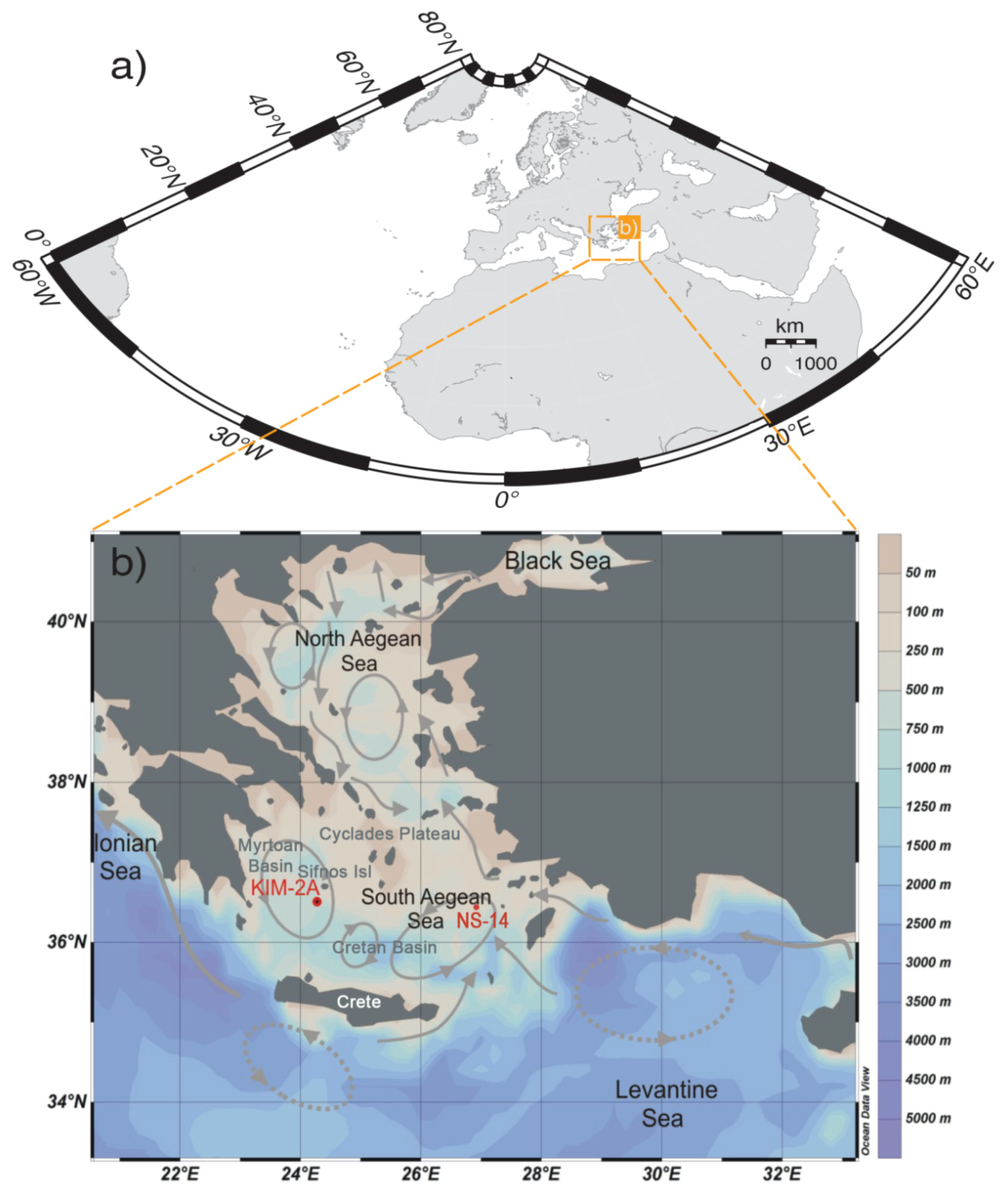
3.1. Location and Sampling Strategy of Core KIM-2A

A gravity core (KIM-2A; 200 cm length) was recovered with R/V Aegaeo in May 2015 from the south Aegean Sea and covers the Late Quaternary (the last ∼21 ka BP). Core KIM-2A was collected from the Cyclades plateau, from a submarine depression (640 m water depth) located north of Kimolos Island (36°95.464′N, 24°06.354′E), as shown in Figure 1b. After splitting, the half core was stored as archival material, whereas the working half has been sampled for multiple analyses (micropaleontology, sedimentology, and geochemistry).
Fifty-eight samples were taken and used for paleontological (planktonic foraminifera and pteropods) and geochemical (Total Organic Carbon; TOC, stable oxygen and carbon isotopes; δ18O, δ13C) analyses between 196 cm and 4 cm. Samples were taken throughout the core but with different sampling resolutions. For the first gray interval corresponding to S1a, the sampling resolution was 1 cm; beyond these intervals the sampling was 2 cm, whereas the top 40 cm were sampled at a mean 8 cm resolution.

3.2. Micropaleontological Analyses

All samples were prepared following standard micropaleontological procedures. For the faunal analyses, approximately 3 cm3 of dried sediment was washed and sieved through a 63 μm screen, and residues were dried in an oven at 50 °C. Qualitative and quantitative analyses have been performed on both planktonic foraminiferal and pteropod assemblages for the >125 μm size fraction, split into aliquots, each one containing at least 300 specimens. It should be noted that the 125 μm fraction was selected since is the most common studied fraction in relevant investigations within the Aegean Sea, which analyze the Late Quaternary foraminiferal record [10,18,21,32,36], and implement a paleoclimatic analysis [6,15,20,72]. All shells were handpicked, identified following [73], counted in each sample, and then converted into percentages, based on the extrapolation of a counted split. Planktonic species with phylogenetic affinities and similar ecological characteristics [35,74] were counted together and grouped to better interpret distribution patterns. On this regard, all Globigerinoides ruber morphotypes (“Normal,” “Platys,” “Elongate,” and “Twin” types; [32]) were plotted together, distinguishing only the “alba” and “rosea” varieties due to their different ecological characteristics [75]. Furthermore, Globigerina bulloides group includes the species G. bulloides and Globigerina falconensis, the Globigerinoides sacculifer group includes Globigerinoides trilobus and G. sacculifer, and the Globigerinella siphonifera group includes the species Globigerinella aequilateralis, Globigerina calida, and Globigerina digitata. The species Globigerinita glutinata includes the morphotypes with and without bulla. Within the group of Neogloboquadriniids, two types were discerned: Neogloboquadrina pachyderma and Neogloboquadrina dutertrei.

3.3. Total Organic Carbon and Stable Isotopes

Total organic carbon (TOC) was determined based on the [76] methodology with the [77] adaptation at the Laboratory of the Hellenic Survey of Geology and Mineral Exploration (H.S.G.M.E.). For stable oxygen and carbon (δ18O, δ13C) isotope measurements, 30 specimens of the planktonic species G. ruber f. alba were picked from the 250–300 μm size fraction. In particular, we exclusively used the morphotype “Normal” of [32] (equivalent to G. ruber sensu stricto [75]) in order to minimize potential morphotype-specific differential responses in stable isotope compositions [24,78,79]. This narrow size fraction was used to minimize ontogenetic and growth rate effects on shell geochemistry [80]. The analyses were carried out at the Laboratory of Geology and Geophysics at Edinburgh University. Foraminiferal δ18O and δ13C data were calibrated to National Bureau of Standards 19 (NBS19), and the isotope values are reported in ‰ relative to Vienna Pee Dee belemnite scale. The external standard errors of the stable carbon and oxygen isotope analyses are <0.06‰ and 0.08‰, respectively.

3.4. Chronology

The chronology of the core KIM-2A is based on five accelerator mass spectroscopy radiocarbon (AMS 14C) dates (on G. ruber tests at Beta Analytics laboratories), supplemented by tie-points which correspond to well-dated bio-litho-stratigraphic horizons (e.g., sapropel and planktonic foraminiferal biozone boundaries) from nearby Aegean cores (Table 1). Conventional 14C ages were calibrated by means of the Calib version 7.0.2 software [81] and the Marine13 data set with a regional reservoir age correction (ΔR) of 139 ± 40 years for the S1 interval [82] and of 58 ± 85 years outside the sapropel S1 interval [83]. The chronology adopted in this study for core KIM-2A was derived from a polynomial fit through the calibrated dates and the chronostratigraphic control points’ dating as shown in Table 1. Hereafter, ages in this study are reported in calibrated thousands of years before present, notated ka BP.

3.5. Multivariate Statistical Analyses

Principal component analyses (PCA) is used to reduce the dimensionality of a multivariate data set to a few principal factors that determine the distributions of species. For this analysis all raw data for the totality of the samples and specimens were used. Raw data were processed using PAST (2.17) multivariate statistical software package of [85]. The resulting factor scores show the contribution of each factor in every sample, and therefore the down-core contribution of each factor. The total number of factors was defined by minimizing the remaining “random” variability, and by the possibility to relate the factors to modern hydrographic conditions and planktonic foraminiferal and pteropod ecology.

3.6. Paleoceanographic Indices

The planktonic foraminiferal relative distributions were used as a first-order estimate of sea-surface temperature (SST) variations. An index of the SST variations was constructed based on the down-core variation of planktonic foraminiferal abundances, referred to as planktonic paleoclimatic curve (PPC). The PPC was obtained by the formula 100 × (w − c)/(w + c), where w represents the warm-water indicators (G. ruber f. alba, G. ruber f. rosea, Orbulina universa, G. sacculifer gr., Globoturborotalita rubescens, and G. siphonifera gr.), and c the cold-water indicators (Globorotalia inflata, Globorotalia truncatulinoides, Turborotalita quinqueloba, G. glutinata, and Globorotalia scitula). The eutrophication index (E-index; [7]) was estimated using the sum of the eutrophic species (N. pachyderma, N. dutertrei, G. bulloides, T. quinqueloba, and G. inflata) versus the sum of the eutrophic plus oligotrophic species (G. ruber alba, G. ruber rosea, G. rubescens, G. sacculifer, O. universa, and G. siphonifera). The down-core ratio between G. bulloides and G. ruber was also estimated showing the degree of the stratification of the upper water column [86]. Following [7], this ratio is referred to as S-index, and its values reflect periods of strong summer stratification of the water column where oligotrophic taxa dominate (low values) and/or periods of strong winter mixing of the water column where eutrophic taxa dominate (high values).

4. Results

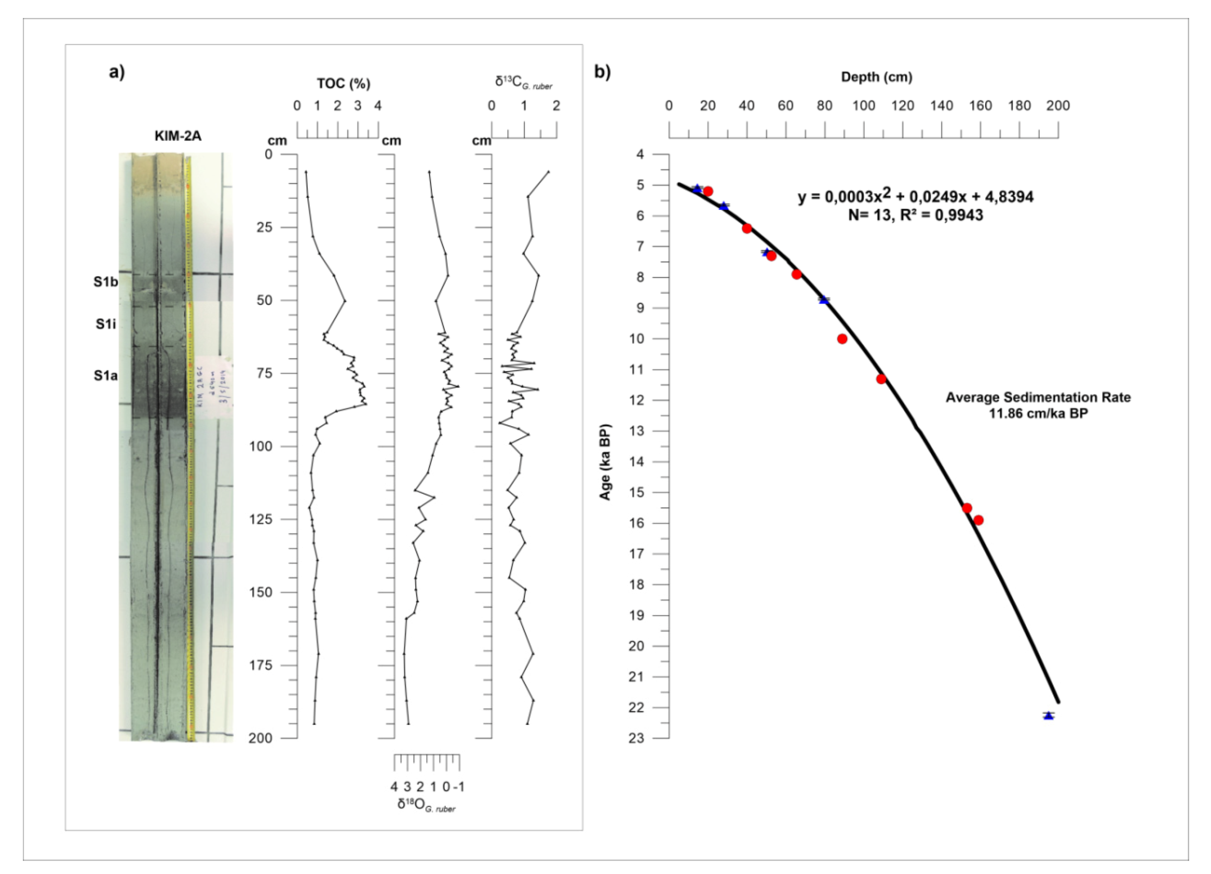
4.1. Lithological Description, Time Stratigraphic Framework, and Sedimentation Rates

Lithologically, the study core contains a distinct organic-rich dark interval, divided into two separate sub-units (S1a and S1b respectively), representing the regional expression of the most recent sapropel S1 [87,88] (Figure 2a). From the bottom up to 87.5 cm, light gray clay can be observed (Munsell soil color 5Y 7/1). The following 24 cm are of gray color (5Y 5/1) and correspond to the lower sub-unit (S1a) of the sapropel. Between 63.5 cm and 52 cm light gray clay (5Y 7/1) can be observed, indicative of the sapropel interruption (S1i). From 52 cm to 40 cm mud of gray color (5Y 5/2) characterizes the upper sapropel sub-unit (S1b). The clay continues up to 13.5 cm with a light gray clay (5Y 7/1) color. From this point to the top of the core watery clay of light-yellow color (5Y 7/4) can be observed (Figure 2a).
Chronology adopted in this study for core KIM-2A derived from a polynomial fit through the five AMS 14C datings mentioned above, and the time markers correlative to the start and end of sapropel deposition, as well as the planktonic foraminiferal biozone Ia/Ib, Ib/Ic, Ic/II and II/III boundaries of [84] in the Mediterranean Sea (Table 1). The resulting age model is illustrated in Figure 2b and is consistent with the multi-proxy chronological framework of [37] for the Aegean sediment cores, thus supporting the robustness of our chronology. For the ages of the onset and termination of sapropel deposition, we have used the relevant ages from the nearby core NS-14 [7,16,17]. Additional control points related to the planktonic foraminiferal biozone boundaries were used for the age model construction, since they are useful chronologic standards for dating late Quaternary sequences in the central and eastern Mediterranean (including the Aegean Sea; [6,7,52,89] due to their Mediterranean-wide applicability and synchroneity [90,91,92].
Based on the relative abundances of the planktonic foraminifera species (Figure 3) the interval between 196 cm and 153 cm is characterized by the dominance of N. pachyderma, T. quinqueloba, G. scitula and G. glutinata with additional components the species G. ruber f. alba and G. bulloides. This glacial fauna corresponds to assemblage III and it has been recognized throughout the Mediterranean Sea (e.g., [6,52]). The interval between 153 cm and 109 cm corresponds to assemblage II and is characterized by high relative abundances of Neogloboquadrinids and G. glutinata and the presence of and G. inflata. In the lower part of this interval G. ruber f. rosea appears for the first time. Subzone Ic (109–40 cm) was identified by the warm subtropical species (G. ruber f. rosea, G. siphonifera gr. and O. universa). In addition it includes abundant G. bulloides and G. rubescens specimens. The sharp increase in the abundance of G. inflata at 41.5 cm is inferred to mark the onset of the Ib subzone. The Ia/Ib boundary (at 20 cm) is marked by the decrease of the latter species along with the decrease in the N. pachyderma abundance. In this core the Bioevent “Start of δ18Oruber depletion T1a” of [52], was also detected at 159 cm.
According to our proposed age model (Figure 2b), the sedimentary horizons sampled in this study span the interval from the late glacial period, and the subsequent transition (Termination 1; T1) to the middle Holocene (Northgrippian stage) (i.e., ~5–22 ka BP). The average sedimentation rate is 11.86 cm/ka, and is in good agreement to those reported in the marginal Aegean basin [4,7,13,52]. These sedimentation rates were derived from the age model, assuming that the sediment accumulation has been moderately consistent throughout each interval. In particular, the average sedimentation rates are 8.10 cm/ka for the late glacial, 10.30 cm/ka for the Termination T1, and 16.46 cm/ka for the Holocene.

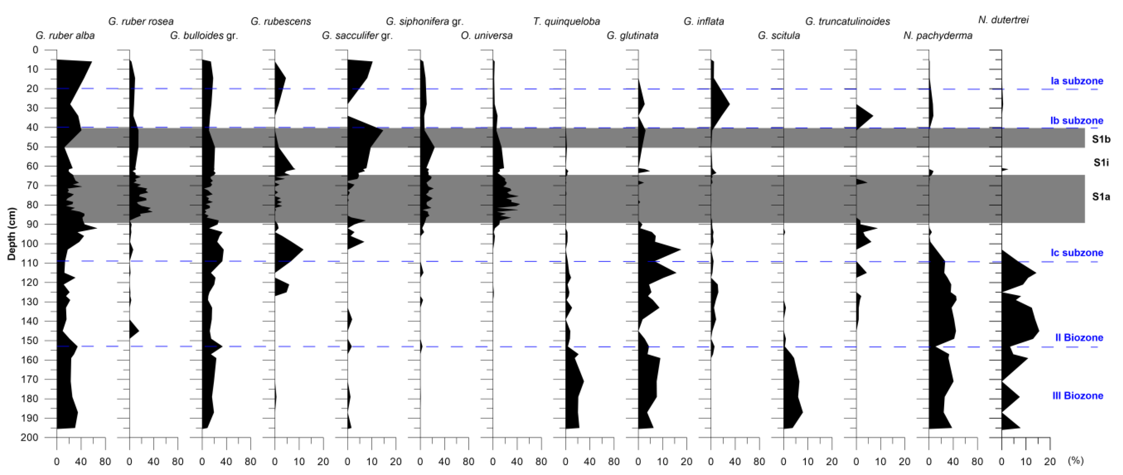
4.2. Planktonic Foraminifera Distribution Pattern

The qualitative analysis revealed 19 planktonic foraminiferal species lumped into 14 groups: G. ruber f. alba, G. ruber f. rosea, G. sacculifer group, G. bulloides group, G. siphonifera group, G. scitula, G. truncatulinoides, G. inflata, O. universa, T. quinqueloba, G. glutinata, G. rubescens, N. pachyderma, N. dutertrei. The down-core stratigraphic distributions of their relative abundance are shown in Figure 3.
From the bottom of the core up to 153 cm, the fauna is characterized by high relative abundances of the species G. ruber f. alba (22–34%), N. pachyderma (10–40%), T. quinqueloba (3–30%), and G. bulloides gr. (8–33%). Additional components of the fauna are N. dutertrei, G. glutinata, and G. scitula. After the 153 cm, an abrupt decline in Neogloboquadrinids and T. quinqueloba can be observed, while G. bulloides follows an opposite trend with relative abundance of 33%. From that point up to 127 cm N. pachyderma and N. dutertrei reach their maximum abundances (45% and 15% respectively), whereas T. quinqueloba is still present but with low percentages (up to 10%). The relative abundance of G. bulloides does not exceed 16% and G. ruber f. alba is also present but with equally low frequency (lower than 20%). Between 127 cm and 100 cm the fauna is characterized by the dominance of G. bulloides, N. pachyderma, N. dutertrei, G. ruber f. alba, G. glutinata, and G. rubescens. Additional components, with lower percentages, are the species T. quinqueloba and G. inflata. The interval between 100 cm and 41.5 cm is characterized by a shift in fauna. Most of the species dominating the previous interval are decreasing or becoming absent (T. quinqueloba, Neogloboquadrinids, G. glutinata and G. inflata). Prevailing species of this interval are O. universa (44%), G. ruber f. rosea (38%), G. bulloides gr. (27%), G. siphonifera gr. (20%), and G. sacculifer gr. (14%). In the final segment of the core, from 41.5 cm to the top, the sampling presents poor resolution, but certain significant changes can be observed. The G. ruber f. alba, G. inflata and G. truncatulinoides present a peak (57%, 31%, and 7% respectively) and the relative abundances of G. ruber f. rosea, O. universa, and G. siphonifera gr. are decreasing. N. pachyderma, G. inflata, and G. glutinata are re-appearing, but with low percentages.

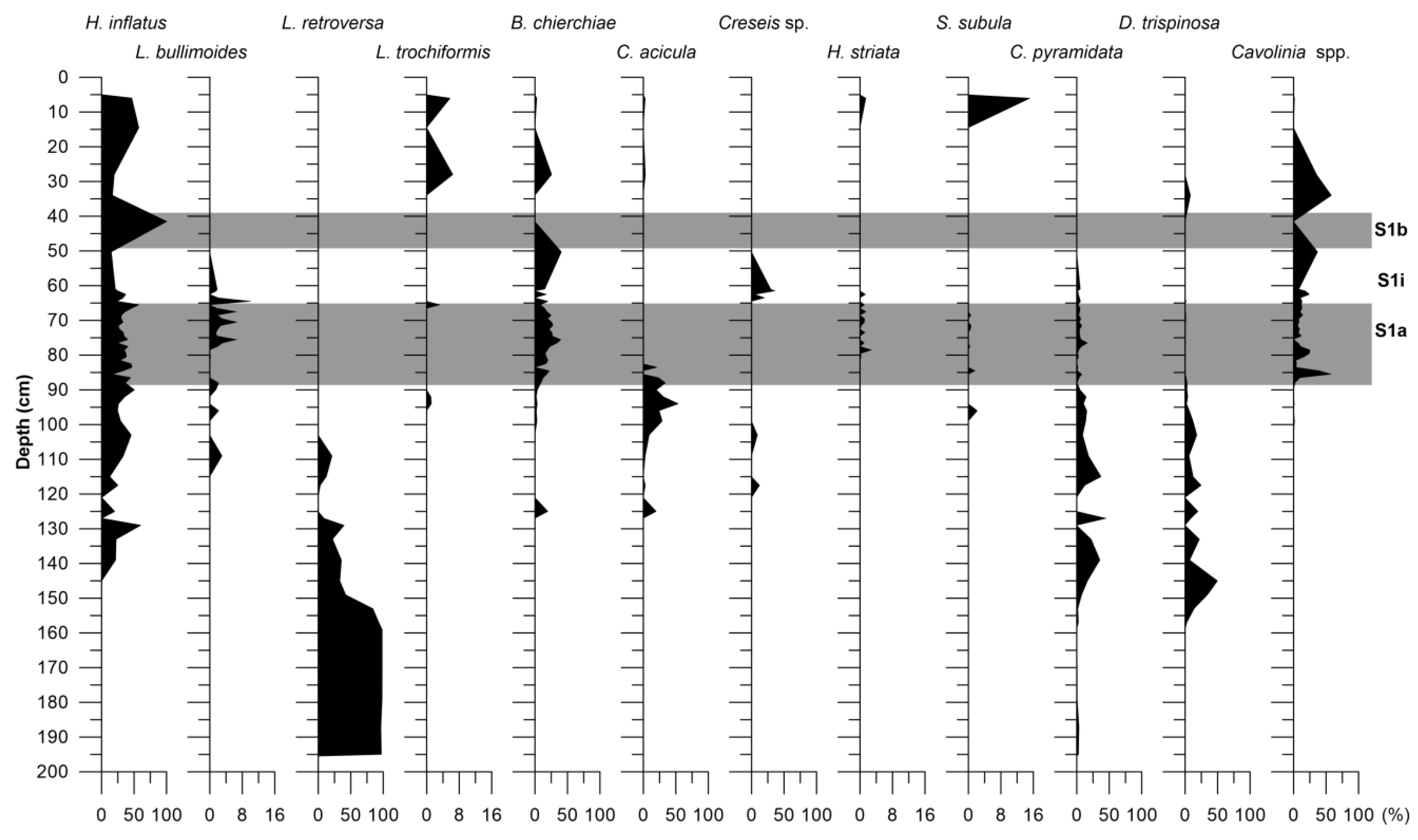
4.3. Pteropod Distribution Pattern

All samples examined for foraminifera include significant amounts of aragonitic pteropods indicating excellent preservation (without any signals of dissolution) along with the strong carbonate preservation potential of the eastern Mediterranean basin [72,93]. A total of 12 species of Euthecosomata (Heliconoides inflatus, Limacina trochiformis, Limacina bulimoides, Limacina retroversa, Creseis acicula, Creseis sp., Boasia chierchiae, Hyalocyclis striata, Styliola subula, Clio pyramidata s.l., Diacria trispinosa, Cavolinia spp.) were identified. Adult specimens, when present, were fragmented (Cavolinia spp., C. pyramidata). The protoconchs (Clio, Diacria and Cavolina) made the identification of certain species and genera possible, as they were the only residue left. The down-core variation of their abundance is presented in Figure 4.
Within the basal part of the core sequence, the fauna is composed almost exclusively of the pteropod L. retroversa. An additional component is the species C. pyramidata, but with very low percentages (<3.5%). Between 153 cm to 127 cm the pteropodal fauna becomes more diverse with the species H. inflatus, D. trispinosa, C. acicula, and B. chierchiae appearing in the fauna. The relative abundance of C. pyramidata gradually increases (up to 45%), in contrast to the decline of L. retroversa (drops to ~40%). The latter disappears completely from the fauna at 105 cm. Between 109 cm and 85 cm the pteropod fauna consists mainly of H. inflatus, C. acicula, C. pyramidata, and D. trispinosa, with L. bullimoides appearing for the first time at 109 cm. The species C. pyramidata and D. trispinosa are exponentially decreasing untill, and including, the top of the core sample. In the last 85 cm of the core, Cavolinia spp. appears in the fauna, reaching its maximum abundance (58%) at 41.25 cm and 85.5 cm, with the species H. inflatus and B. chierchiae (15–58% and 3–40% respectively) as additional components. At 65.5 cm, L. trochiformis presents a short occurrence and between 65 cm and 60 cm Creseis sp. presents its maximum relative abundance (36%). Towards the top of the core L. trochiformis and S. subula present their highest percentages (~6% and 15% respectively).

4.4. Total Organic Carbon and Stable Isotopes

Total organic carbon (TOC) in KIM-2A generally exhibits values around 1%. This pattern is interrupted in two intervals related to the sapropel sub-units deposition. The first interval (S1a; 89–64 cm) is characterized by high TOC concentration, ranging from 1.5% to 3.4%, and in the second interval (S1b; 52.5–40 cm), TOC concentration ranges from 1.8% to 2.4% (Figure 2a). Thus, the deposition of S1 sapropel layer started at 89 cm and terminated at 40 cm. The interruption of sapropel S1 layer (S1i) is detected between 64 cm and 52.5 cm, as suggested by the TOC content (~1.3%).
As shown in Figure 2a, between 196 cm and 159 cm, δ18OG. ruber values range from +2.9 to +3.2‰. From 157 cm to 115 cm, a depletion in δ18OG. ruber values is observed (up to +0.9‰) and persists until the 34 cm with even lower values. More precisely, the depleted values were recorded from two intervals (88.5–65.5 cm and 50.25–34 cm) with an average value of −0.08‰ and +0.25‰ respectively. In the interval corresponding to 66.5–61 cm, slightly heavier δ18OG. ruber values were observed (+0.6 to −0.1‰). In the final unit of the core, from 28 cm until the top, a core enrichment in δ18OG. ruber is recorded. The δ13CG. ruber values of KIM-2A core exhibit more scatter than the δ18O records. In the basal part of the core (200–88 cm) values range between +1.3 to +0.2‰. In the interval between 88 cm and 61 cm the δ13CG. ruber ranges between 0.3 and 0.9‰ with the exception of three high-positive peaks at 80.5 cm, 73.5 cm, and 71.5 cm with values of 1.4‰, 1.2‰, and 1.3‰ respectively. From 50.25 cm to the top of the core, δ13CG. ruber exhibits heavier values with an average of +1.29‰ (Figure 2a).

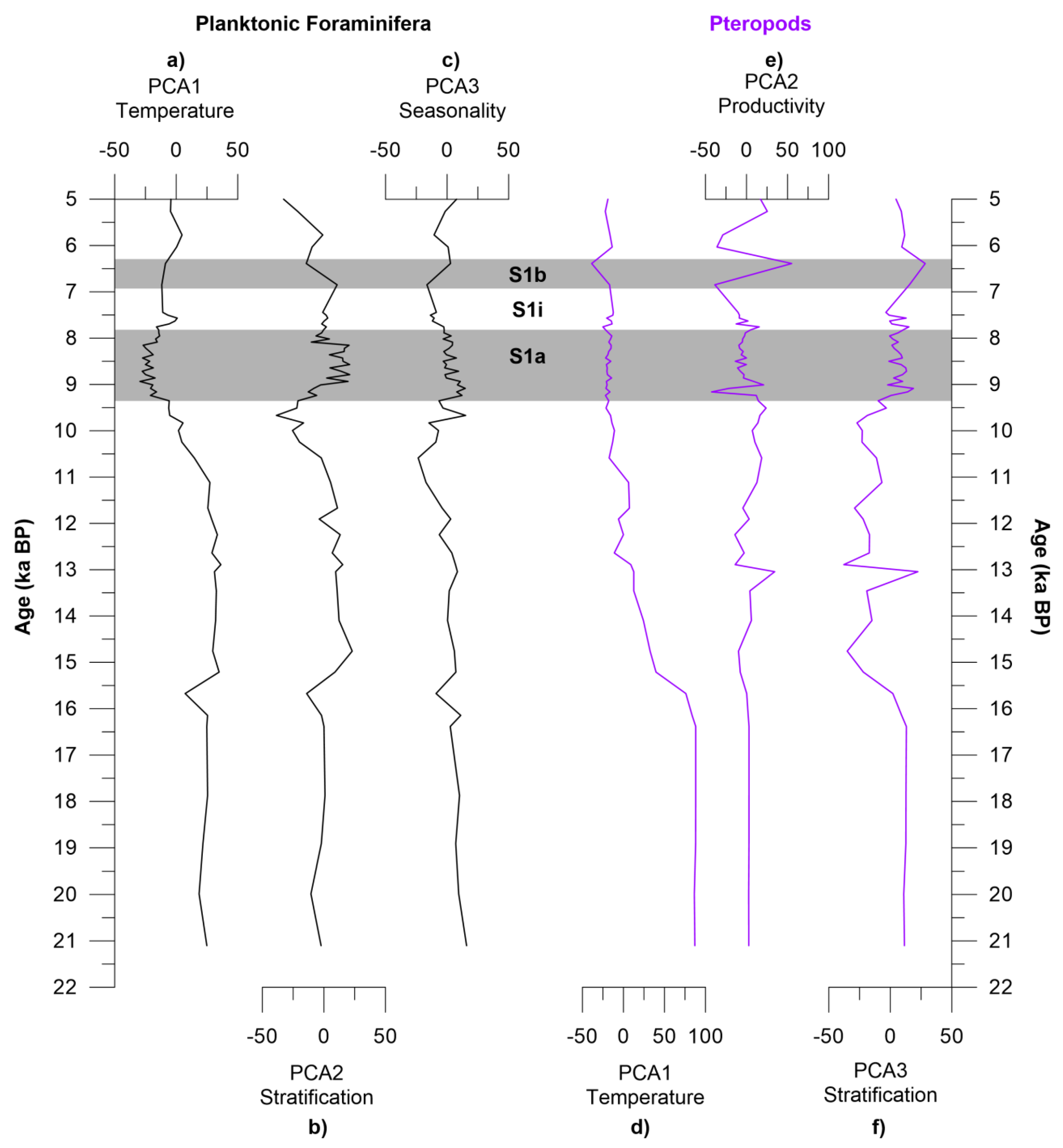
4.5. Principal Component Analysis

A standardized principal component analysis (PCA) was carried out on the total data set using the varimax method, in order to determine the impact of various environmental parameters on the planktonic distribution. The application of this statistical analysis yielded a three-factor model for both planktonic foraminiferal and pteropod communities (Supplementary Materials; including PCA scores and biplots). The interpretation of the three components in each case was based on the screen plots of eigen values, and the factor loadings of the planktonic foraminiferal and pteropod species respectively. The 3 distinguished factors were considered to account for 81.57% and 82.81% of the total variance in each category respectively (Table 2 and Table 3), with their factor loadings showing the contribution of each factor in every sample and therefore the downcore contribution of each factor (Table 4 and Table 5; Figure 5). In the case of a bipolar factor, which has extremes of positive and negative loadings, high positive factor scores are related to the positive pole and high negative scores to the negative pole, respectively.

4.5.1. Planktonic Foraminifera

The first varimax factor (PCA1; Figure 5a) accounts for 50.26% of the total variance (Table 2) and is interpreted as temperature indicator. Species with positive loadings (N. pachyderma, T. quinqueloba, N. dutertrei, G. glutinata, G. inflata, G. bulloides, and G. scitula; Table 4) thrive in cold–water masses, while the species with negative loadings (O. universa, G. ruber f. rosea, G. siphonifera gr., and G. ruber f. alba; Table 4) thrive in warm–water conditions. Factor PCA2 (Figure 5b) accounts for 22.5% of the total variance (Table 1), with the positive pole being expressed by species living in a highly stratified water column (O. universa, G. ruber f. rosea and Neogloboquadrinids) and negative pole by species typical of the weak development of these conditions (G. ruber f. alba and G. bulloides gr.). The third varimax factor (PCA3) describes 8.9% of the total variance (Table 2), and also display a bipolar character, with its positive pole to be represented mainly by G. ruber f. alba and N. pachyderma and the negative pole by G. bulloides. The above species that characterize the PCA3 factor are the main exponents of the seasonal contrasts governing planktonic foraminiferal assemblages in the Mediterranean Sea during the last glacial cycle [94,95,96]. Thus, the third varimax factor (PCA3; Figure 5c) is referred to as a seasonality factor.

4.5.2. Pteropods

The first varimax factor (PCA1; Figure 5e) accounts for 58.66% of the total variance (Table 3) and was interpreted as a temperature indicator. Negative loadings consist mainly of the warm–water species H. inflatus, whereas positive loadings consist mainly of the subarctic species L. retroversa (Table 5). The second factor (PCA2; Figure 5e) describes 13.29% of the total variance (Table 3) and was interpreted as a productivity factor, as its positive pole is represented mainly by the mesopelagic oligotrophic H. inflatus. The third varimax factor (PCA3; Figure 5f) explains 10.27% of the total variance (Table 3). The positively loading taxa expressed by the epipelagic Cavolinia sp., L. retroversa and B. chierchiae, as well as the mesopelagic and tolerant to low oxygen concentration H. inflatus, whereas the negatively loading taxa (mesopelagic C. pyramidata and D. trispinosa) prefer a well-ventilated water column (Table 5). Thus, the third factor (PCA3) can be regarded as a stratification factor.

5. Discussion

5.1. Factors Controlling Planktonic Fauna Distribution in the Aegean Sea

Of the oceanographic factors typically considered, SST shows the highest explanatory power for the distribution of the planktonic fauna during the Late Quaternary. This is in accordance with previously published studies showing temperature as the dominant factor controlling the biogeography of planktonic foraminifera and pteropods at both global and local scales [61,67,97]. However, the 2 remaining factors (PCA-2, PCA-3) exhibit a bipolar character and could be considered as indicators of the annual stability of the water column. For the planktonic foraminifera fauna, they show that the faunal composition in the south Aegean Sea was not only controlled by SST, but also seems to be affected by the degree of development and location of a permanent or seasonal thermocline/pycnocline. Its vertical placement in the water column is a direct consequence of changes in sea surface salinity (SSS) and productivity (SSP), which ultimately reflected the seasonal fluctuations of the periods of vertical mixing of water in the periods of intense stratification. The interpretation of the second axis focused on the appearance depths of pycnocline and deep chlorophyll maximum (DCM) and the thickness of mixed layer. The interpretation of the third axis focused on upwelling currents and/or river inputs (e.g., G. bulloides), parameters which primarily control the food availability and reproductive cycles of foraminifera [73] and are directly correlated to the seasonal fluctuations they present [94,98,99,100]. Therefore, a useful additional dimension of planktonic foraminifera ecology that is underlined by the PCA conducted in this study is the degree of vertical stratification of the water column and the way it is recorded (seasonal presence/absence pycnocline and DCM and upwellings and runoff), which are inextricably linked with the factors of primary productivity and seasonality. Similarly, the second and third factor (PCA2, PCA3) of pteropods are focused on the hydrological conditions and the overall oxygenation of the water column. Particularly, the down-core scores of the second factor coincide with the δ13C and E-index values, indicating that variations in primary productivity have an impact on pteropod abundances. Even though nutrient concentrations are not a limited factor for their distribution [67], our data suggest that fluctuations in nutrients and salinity due to the increased freshwater inputs during the sapropel deposition favor the flourishment of some species (Cavolinia spp., B. chierchiae; Figure 4). Additionally, the third factor suggests that oxygen concentration, and thus the intensity of the oxygen minimum zone (OMZ), are parameters that affect pteropod distribution and particularly the mesopelagic species [66].

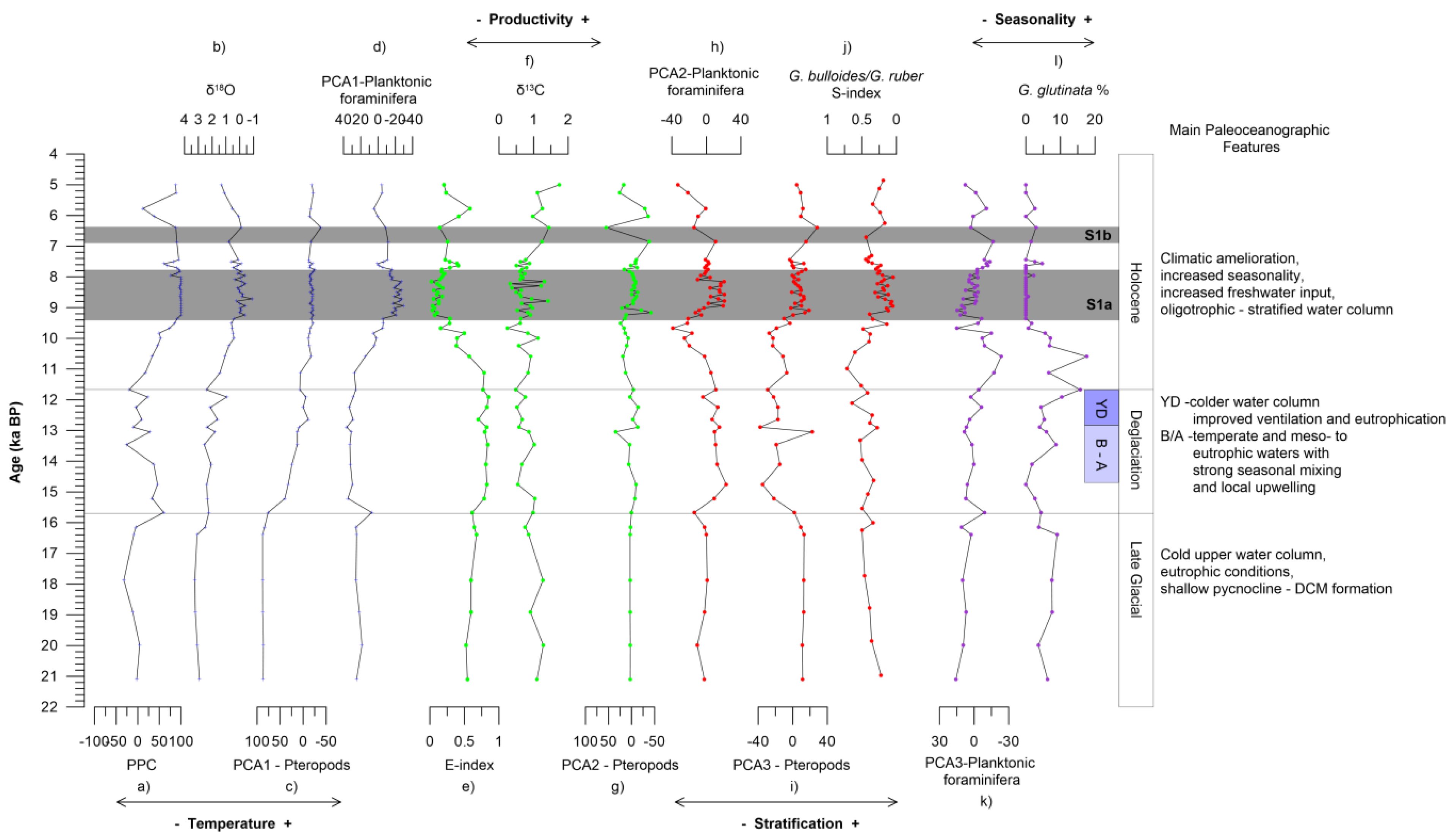
5.2. Paleoceanographic Reconstruction

The results of the multivariate statistical analyses, in combination with paleoceanographic indices and isotopic data (Figure 6), reveal a succession of Late glacial to Holocene paleoclimatic and paleoceanographic changes. The evidence of these changes is interpreted and discussed in terms of the events that mainly accompanied the transition out of the late glacial period and the deposition of sapropel S1 during the Holocene Climatic Optimum (HCO).

5.2.1. Late Glacial

During the late glacial period (21.1–15.7 ka BP), the heaviest δ18O values (2.49–3.26‰), accompanied by relatively low PPC values (−32% to +4%), suggest a cold upper water column (Figure 6a,b). Particularly, this interval was characterized by high percentages of the cold water foraminifera species T. quinqueloba (~30%), accompanied by G. glutinata (9%), and G. scitula (8%), and significant percentages of the warm-water G. ruber f. alba (~34%), that are suggestive of milder climate after the Last Glacial Maximum (LGM), which is in accordance with other records in the Mediterranean [101,102]. Pteropod fauna is composed mainly by the cold water species L. retroversa (98%) and the cold-tolerant mesopelagic C. pyramidata in very low percentages (3%) which is consistent with relevant late glacial Mediterranean records [33,61,103]. Eutrophic species are also abundant in this interval (N. pahyderma, N. dutertrei, T. quinqueloba and G. bulloides) and are associated with the high values of E-index (Figure 6e). Notably, the high abundance of N. pachyderma (26%) indicates shallowing of the pycnocline and the formation of a DCM layer. In addition, δ13C values, around +1‰, and the trend to higher S-index values (Figure 6f,j), also support the development of eutrophicated waters. The moderate abundance of G. bulloides (5−17%; Figure 3) suggests little to no upwelling and/or runoff contribution in primary productivity. Therefore, the injection of nutrients into the euphotic zone can be attributed to the intensification and southward shift of westerly winds, as indicated by atmospheric circulation models for this time interval [104].

5.2.2. Deglaciation

At 15.7 ka BP an abrupt shift of PPC to positive values, accompanied by lighter δ18O values (+2.2‰) (Figure 6a,b), are indicative of the climatic amelioration that occurred during the last deglaciation. These warmer conditions are also supported by the occurrence of the warm water species H. inflatus and D. trispinosa (up to 60% and 50% respectively), and the decrease in L. retroversa percentages (between 33% and 85%). This warming trend is in agreement with relevant paleoclimatic records from the eastern Mediterranean, and is attributed to the Bølling–Allerød (B-A) interstadial [7,13,14,105,106]. The increased SST and humidity are also recorded by the higher abundance of the terrestrial biomarkers in the south Aegean [17], and by a change in the benthic faunas from oxic to dysoxic indicator species [13]. In the beginning of this interval, Neogloboquadrinids were temporarily replaced by G. bulloides (26%), suggesting local upwelling. Though, later on the eutrophic N. pachyderma and N. dutertrei present their highest abundance (42% and 14% respectively). Additional components of this interval are G. ruber (both variants), G. bulloides, T. quinqueloba, and G. inflata, suggesting temperate and meso- to eutrophic waters, with strong seasonal mixing and local upwelling.
This state persisted until the onset of the Younger Dryas (YD) at about 12.9 ka BP, which is depicted in the abrupt decrease in PPC (from +28% to −10%) and in heavier values of δ18O (1.0–2.5‰) (Figure 6a,b). The planktonic foraminiferal fauna shows an increase in cold water species (N. pachyderma, T. quinqueloba, G. inflata and G. glutinata). Pteropod fauna is composed mainly of the cold-water species epipelagic L. retroversa and the mesopelagic temperate to warm-water species C. pyramidata and D. trispinosa, while the warm-water H. inflatus presents a decreasing trend (Figure 3). This climate response of south Aegean depression to the YD event (12.9–11.7 ka BP) seems to be in accordance with relevant signals from other Aegean sub-basins [6,7]. Towards the end of YD (12.6–12.2 ka BP) the species G. rubescens, C. acicula, and B. chierchiae are added to the fauna suggesting that mild climatic conditions prevailed for a brief time interval of about 400 years within the YD event. This brief climatic amelioration in the mid YD, which has been attributed to the displacement of the polar front by a few degrees north [26], has been also observed in north-central Aegean marine records [7,106] and coincides with the pattern of GRIP and NGRIP ice-core records [107,108], pollen-based reconstructions from the Jura [109] and the Balkans [110], as well as chironomid-based reconstructions from North Italy [111]. The increases in the S-index and E-index at around 12.2 ka BP (Figure 6e,j) coincide with this amelioration, reflected by the improved ventilation and eutrophication of the water column.

5.2.3. Holocene

With the ending of the YD, a general climatic amelioration is seen in the records (increase in PPC, lighter values in δ18O, decline of temperature factors PCA1; Figure 6a–d) marking the beginning of the Holocene. Planktonic foraminifera fauna consists mainly by G. ruber f. alba that increases in abundance towards the onset of sapropel deposition, along with G. bulloides and N. pachyderma. The two latter species present an opposite trend, decreasing towards the onset of sapropel deposition. This trend suggests the gradual development of stratified and oligotrophic surface waters. Pteropod fauna follows a similar pattern with the decreasing abundances of the species D. trispinosa and C. pyramidata, which are indicative of a well ventilated water column [112], and the increase in the epipelagic B. chierchiae and C. acicula (Figure 4). The reduction of E-index along with the values of δ13C and the S-index (Figure 6e–j) are further evidence for the development of these conditions. The replacement of G. inflata by G. glutinata (Figure 3) may be tentatively explained in terms of increased seasonality, and of increased freshwater input, which reduced surface buoyancy loss and hence suppressed mixing during the beginning of the Holocene [7]. This was also enhanced by the presence of the epipelagic pteropods (Creseis spp.) that proliferate in low-salinity waters [113], and the seasonality factor (PCA3 of planktonic foraminifera; Figure 6k).
At around 9.4 ka BP, the deposition of sapropel S1 as witnessed by their high organic carbon content (Corg: 1.8–3.3%, Figure 2a), coincided with the start of the overall δ18O depletion (+0.6‰ to −0.9‰; Figure 6b). The changes of the planktonic foraminifera fauna are characterized by an increase in G. ruber f. rosea, G. ruber f. alba, G. siphonifera and O. universa that are suggestive of extremely warm and stratified conditions (PPC ~100%; PCA1 low values; Figure 6b–d). The lower values of G. bulloides/G. ruber ratio in this interval are also indicative of strongly stratified water column and are in agreement with the stratification factor for both faunas (PCA2 of planktonic foraminifera and PCA3 of pteropod; Figure 6h–j). An increase in temperature and humidity around this time has been documented in all marine and terrestrial pollen records in the eastern Mediterranean region [6,7,14,15,16,114]. This paleoclimate change coincides with the Holocene summer precession-related insolation maximum in the Northern Hemisphere [115], and the monsoon intensification that resulted in a widespread increase in humidity over the Mediterranean region and concomitant increase of freshwater input to the Mediterranean Sea [116,117]. Pteropod fauna is characterized by the dominance of the warm oligotrophic H. inflatus, and the warm epipelagic B. chierchiae, C. acicula, and Cavolinia spp. (Figure 4). Mesopelagic species (C. pyramidata and D. trispinosa) are decreasing dramatically due to the enhanced stratification of the entire water column. Mesopelagic pteropods are affected by the OMZ alterations, which are climatically controlled [63,112]. In the humid and warmer conditions that persisted during the formation of S1, the subsequent stratification of the water column favored a strong and well developed OMZ that probably led to the reduction of mesopelagic species. The presence of the mesopelagic H. inflatus into the sapropel sublayers can be explained by its habitat. More explicitly, this species adopts a variable depth habitat during its growth stages, and it is more susceptible to the low oxygen concentration in the OMZ [63,118,119]. The presence of L. bulimoides in the upper part of S1a, with peaks at 8.4 ka BP, 8.1 ka BP, and 7.9 ka BP (~6%) and its absence in the S1b, suggest that during the end of S1a (8.6–7.7 ka BP) the conditions were more arid than during the onset of S1a (9.4–8.6 ka BP) and the interval of S1b (6.9–6.4 ka BP). In these two phases of S1a, δ13C present a decreasing trend with an average value of +0.8‰ in the first phase and +0.6‰ in the second (Figure 6f).
The warm and stratified conditions favorable for the sapropel deposition were interrupted between 7.7 ka BP and 6.8 ka BP. This interval (S1i) is marked by the decrease in PPC (from 90% to 60%) and the heavier values of δ18O (+0.5‰) and δ13C (+0.8‰) as shown in Figure 6a,b,f. The subsequent cooling is also reflected in significant faunal changes, such as the increase in abundance of G. inflata, T. quinqueloba, G. bulloides, and N. pachyderma (Figure 3). These species are associated with relatively cold temperatures and increased food supply, suggesting high primary production and stronger mixing of the water column [46,52]. In addition, the pteropod L. trochiformis, which is related to the mixed layer of the water column and thrives in upwelling conditions [120,121,122,123], presents a peak at the beginning of S1i (Figure 4).
From 6.4 ka BP to the top of the core (~5.0 ka BP), a trend to heavier δ18O values (from 0‰ to +1.3‰) and the drop of PPC (~60%) are recorded (Figure 6a,b). In planktonic foraminifera fauna an increase in G. inflata, G. truncatulinoides and N. pachyderma along with the reduction of G. ruber f. rosea, G. siphonifera gr. O. universa indicate lower SST, and stronger seafloor oxygenation due to vertical mixing. This latter is also suggested by the increase in the mesopelagic pteropod D. trispinosa. The peak of L. trochiformis at 5.7 ka BP (Figure 4) is suggestive of upwelling conditions. At this point, and up to 5.0 ka BP, increased percentages of G. bulloides and G. sacculifer are indicative of increased productivity. This is also indicated by the high values of E-index, the heavy δ13C (up to +1.7‰) and the PCA2 factor of pteropods (Figure 6e–g).

6. Conclusions

The results of the analysis of planktonic foraminifera and pteropods, combined with the results of principal component analysis and oxygen and carbon isotopic signals, describe the key factors controlling the formation of the micropaleontological assemblages, and therefore the paleoenvironmental and paleoclimatic changes during the last ~21 ka BP. Our data suggests that the sea surface temperature, stratification of the water column, seasonality, and productivity are the main controlling factors of the faunal distribution. During the Late Glacial, all the records indicate the occurrence of cold and eutrophicated waters. The time interval of 15.9–11.7 ka BP, corresponding to the deglaciation phase, was characterized by gradual climatic amelioration. During this interval, the warm interstadial Bølling–Allerød was identified, while low SST records at 12.9 ka BP revealed the onset of the YD. During this event, mild climate conditions were observed for around 400 years, and are attributed to the displacement of the polar front by a few degrees north. With the onset of the Holocene, a general climatic amelioration can be observed, with the gradual development of stratified oligotrophic surface waters. These conditions were intensified during the sapropel S1 deposition, which appears in two layers (S1a and S1b). The faunal and isotopic data suggest that conditions were more arid towards the end of S1a than at the onset of the S1a and the S1b. The interruption of sapropel deposition (S1i) and the post-sapropel interval are characterized by lower SST and stronger seafloor oxygenation due to vertical mixing.

Supplementary Materials

The following are available online at https://www.mdpi.com/2077-1312/8/9/709/s1, Figure S1: Planktonic foraminiferal PCA biplot of environmental factors of Temperature (Component 1) and Stratification (Component 2), Figure S2: Planktonic foraminiferal PCA biplot of environmental factors of Temperature (Component 1) and Seasonality (Component 3), Figure S3: Pteropods PCA biplot of environmental factors of Temperature (Component 1) and Productivity (Component 2), Figure S4: Pteropods PCA biplot of environmental factors of Temperature (Component 1) and Stratification (Component 3), Table S1: PCA scores based on planktonic foraminifera raw data, Table S2: PCA scores based on pteropods raw data.

Author Contributions

Conceptualization, C.G., G.K.; methodology, C.G., G.K., A.A.; software, C.G., G.K.; validation, C.G., G.K., A.A.; formal analysis, C.G., G.K., A.A.; investigation, C.G.,G.K., C.I., A.A.; resources, C.G., C.I.; data curation, C.G., G.K.; writing—original draft preparation, C.G., G.K.; writing—review and editing, C.G., G.K., E.K., A.A.; visualization, C.G., G.K.; supervision, E.K., A.A.; project administration C.G., A.A.; funding acquisition, E.K., C.I. All authors have read and agreed to the published version of the manuscript.

Funding

This research was funded by EU/ESPA (NSRF; 2007–2013), YPOTHER project (351008) realized at the Institute of Geology and Mineral Exploration recent H.S.G.M.E. E.K. was funded by EU/ESPA (EPAnEK; 2014–2020), INNOVEXPO project (T1EDK-02363). The APC was funded by the Special Account for Research Grants, National and Kapodistrian University of Athens (Grant No. 16599).

Acknowledgments

We wish to thank the captain and crew of R/V Aegaeo (HCMR) for their technical assistance during the YPOTHER cruises, and N. Xirocostas and K. Vallianatou (H.S.G.M.E.) for the organic carbon analysis. We also thank M. Dagla for the English proofreading of the manuscript. Constructive comments by three anonymous reviewers have been essential in improving this manuscript and Victoria Li (Assistant Editor) is thanked for her editorial handling.

Conflicts of Interest

The authors declare no conflict of interest.

References

  1. Zervakis, G.I.; Moncalvo, J.-M.; Vilgalys, R. Molecular phylogeny, biogeography and speciation of the mushroom species Pleurotus cystidiosus and allied taxa. Microbiology 2004, 150, 715–726. [Google Scholar] [CrossRef] [Green Version]
  2. Giorgi, F.; Lionello, P. Climate change projections for the Mediterranean region. Glob. Planet. Chang. 2008, 63, 90–104. [Google Scholar] [CrossRef]
  3. Rohling, E.J.; Grant, K.; Bolshaw, M.; Roberts, A.; Siddall, M.; Hemleben, C.; Kucera, M. Antarctic temperature and global sea level closely coupled over the past five glacial cycles. Nat. Geosci. 2009. [Google Scholar] [CrossRef]
  4. Aksu, A.E.; Yaşar, D.; Mudie, P.J. Paleoclimatic and paleoceanographic conditions leading to development of sapropel layer S1 in the Aegean Sea. Palaeogeogr. Palaeoclim. Palaeoecol. 1995, 116, 71–101. [Google Scholar] [CrossRef]
  5. Roussakis, G.; Karageorgis, A.P.; Conispoliatis, N.; Lykousis, V. Last glacial–Holocene sediment sequences in N. Aegean basins: Structure, accumulation rates and clay mineral distribution. Geo-Mar. Lett. 2004, 24, 97–111. [Google Scholar] [CrossRef]
  6. Geraga, M.; Ioakim, C.; Lykousis, V.; Tsaila-Monopolis, S.; Mylona, G. The high-resolution palaeoclimatic and palaeoceanographic history of the last 24,000 years in the central Aegean Sea, Greece. Palaeogeogr. Palaeoclim. Palaeoecol. 2010, 287, 101–115. [Google Scholar] [CrossRef]
  7. Kontakiotis, G. Late Quaternary paleoenvironmental reconstruction and paleoclimatic implications of the Aegean Sea (eastern Mediterranean) based on paleoceanographic indexes and stable isotopes. Quat. Int. 2016, 401, 28–42. [Google Scholar] [CrossRef] [Green Version]
  8. Lykousis, V.; Chronis, G.; Tselepides, A.; Price, N.B.; Theocharis, A.; Siokou-Frangou, I.; Van Wambeke, F.; Danovaro, R.; Stavrakakis, S.; Duineveld, G.; et al. Major outputs of the recent multidisciplinary biogeochemical researches undertaken in the Aegean Sea. J. Mar. Syst. 2002, 33–34, 313–334. [Google Scholar] [CrossRef]
  9. Poulos, S.E. The Mediterranean and Black Sea Marine System: An overview of its physico-geographic and oceanographic characteristics. Earth Sci. Rev. 2020, 200, 103004. [Google Scholar] [CrossRef]
  10. Kontakiotis, G. Palaeoceanographic and Palaeoclimatic Study of Eastern Mediterranean During Late Quaternary, Based on Planktonic Foraminiferal Assemblages (in Greek, with English extended abstract). Ph.D. Thesis, National and Kapodistrian University of Athens, Athens, Greece, 2012. [Google Scholar]
  11. Poulos, S.E.; Drakopoulos, P.G.; Collins, M.B. Seasonal variability in sea surface oceanographic conditions in the Aegean Sea (Eastern Mediterranean): An overview. J. Mar. Syst. 1997, 13, 225–244. [Google Scholar] [CrossRef]
  12. Geraga, M.; Tsaila-Monopolis, S.; Ioakim, C.; Papatheodorou, G.; Ferentinos, G. Short-term climate changes in the southern Aegean Sea over the last 48,000 years. Palaeogeogr. Palaeoclim. Palaeoecol. 2005, 220, 311–332. [Google Scholar] [CrossRef]
  13. Kuhnt, T.; Schmiedl, G.; Ehrmann, W.; Hamann, Y.; Hemleben, C. Deep-sea ecosystem variability of the Aegean Sea during the past 22 kyr as revealed by Benthic Foraminifera. Mar. Micropaleontol. 2007, 64, 141–162. [Google Scholar] [CrossRef]
  14. Kotthoff, U.; Müller, U.C.; Pross, J.; Schmiedl, G.; Lawson, I.T.; van de Schootbrugge, B.; Schulz, H. Lateglacial and Holocene vegetation dynamics in the Aegean region: An integrated view based on pollen data from marine and terrestrial archives. Holocene 2008, 18, 1019–1032. [Google Scholar] [CrossRef]
  15. Giamali, C.; Koskeridou, E.; Antonarakou, A.; Ioakim, C.; Kontakiotis, G.; Karageorgis, A.P.; Roussakis, G.; Karakitsios, V. Multiproxy ecosystem response of abrupt Holocene climatic changes in the northeastern Mediterranean sedimentary archive and hydrologic regime. Quat. Res. 2019, 92, 665–685. [Google Scholar] [CrossRef]
  16. Triantaphyllou, M.V.; Ziveri, P.; Gogou, A.; Marino, G.; Lykousis, V.; Bouloubassi, I.; Emeis, K.-C.; Kouli, K.; Dimiza, M.; Rosell-Melé, A.; et al. Late Glacial-Holocene climate variability at the south-eastern margin of the Aegean Sea. Mar. Geol. 2009, 266, 182–197. [Google Scholar] [CrossRef]
  17. Triantaphyllou, M.V.; Antonarakou, A.; Kouli, K.; Dimiza, M.; Kontakiotis, G.; Papanikolaou, M.D.; Ziveri, P.; Mortyn, P.G.; Lianou, V.; Lykousis, V.; et al. Late Glacial–Holocene ecostratigraphy of the south-eastern Aegean Sea, based on plankton and pollen assemblages. Geo Mar. Lett. 2009, 29, 249–267. [Google Scholar] [CrossRef]
  18. Drinia, H.; Antonarakou, A.; Tsourou, T.; Kontakiotis, G.; Psychogiou, M.; Anastasakis, G. Foraminifera eco-biostratigraphy of the southern Evoikos outer shelf, central Aegean Sea, during MIS 5 to present. Cont. Shelf Res. 2016, 126. [Google Scholar] [CrossRef]
  19. Koutrouli, A.; Anastasakis, G.; Kontakiotis, G.; Ballengee, S.; Kuehn, S.; Pe-Piper, G.; Piper, D.J.W. The early to mid-Holocene marine tephrostratigraphic record in the Nisyros-Yali-Kos volcanic center, SE Aegean Sea. J. Volcanol. Geotherm. Res. 2018, 366, 96–111. [Google Scholar] [CrossRef]
  20. Antonarakou, A.; Kontakiotis, G.; Zarkogiannis, S.; Mortyn, P.G.; Drinia, H.; Koskeridou, E.; Anastasakis, G. Planktonic foraminiferal abnormalities in coastal and open marine eastern Mediterranean environments: A natural stress monitoring approach in recent and early Holocene marine systems. J. Mar. Syst. 2018, 181, 63–78. [Google Scholar] [CrossRef]
  21. Louvari, M.A.; Drinia, H.; Kontakiotis, G.; Di Bella, L.; Antonarakou, A.; Anastasakis, G. Impact of latest-glacial to Holocene sea-level oscillations on central Aegean shelf ecosystems: A benthic foraminiferal palaeoenvironmental assessment of South Evoikos Gulf, Greece. J. Mar. Syst. 2019, 199, 103181. [Google Scholar] [CrossRef]
  22. Kontakiotis, G.; Mortyn, P.G.; Antonarakou, A.; Martínez-Botí, M.A.; Triantaphyllou, M.V. Field-based validation of a diagenetic effect on G. ruber Mg/Ca paleothermometry: Core top results from the Aegean Sea (eastern Mediterranean). Geochem. Geophys. Geosyst. 2011, 12. [Google Scholar] [CrossRef]
  23. Kontakiotis, G.; Karakitsios, V.; Mortyn, P.G.; Antonarakou, A.; Drinia, H.; Anastasakis, G.; Agiadi, K.; Kafousia, N.; De Rafelis, M. New insights into the early Pliocene hydrographic dynamics and their relationship to the climatic evolution of the Mediterranean Sea. Palaeogeogr. Palaeoclim. Palaeoecol. 2016, 459, 348–364. [Google Scholar] [CrossRef]
  24. Antonarakou, A.; Kontakiotis, G.; Mortyn, P.G.; Drinia, H.; Sprovieri, M.; Besiou, E.; Tripsanas, E. Biotic and geochemical (δ18O, δ13C, Mg/Ca, Ba/Ca) responses of Globigerinoides ruber morphotypes to upper water column variations during the last deglaciation, Gulf of Mexico. Geochim. Cosmochim. Acta 2015, 170, 69–93. [Google Scholar] [CrossRef]
  25. Le Houedec, S.; Mojtahid, M.; Bicchi, E.; de Lange, G.J.; Hennekam, R. Suborbital Hydrological Variability Inferred From Coupled Benthic and Planktic Foraminiferal-Based Proxies in the Southeastern Mediterranean During the Last 19 ka. Paleoceanogr. Paleoclimatol. 2020, 35, e2019PA003827. [Google Scholar] [CrossRef]
  26. Cacho, I.; Grimalt, J.O.; Canals, M.; Sbaffi, L.; Shackleton, N.J.; Schönfeld, J.; Zahn, R. Variability of the western Mediterranean Sea surface temperature during the last 25,000 years and its connection with the Northern Hemisphere climatic changes. Paleoceanography 2001, 16, 40–52. [Google Scholar] [CrossRef]
  27. Filippidi, A.; Triantaphyllou, M.; de Lange, G. Eastern-Mediterranean ventilation variability during sapropel S1 formation, evaluated at two sites influenced by deep-water formation from Adriatic and Aegean Seas. Quat. Sci. Rev. 2016, 144, 95–106. [Google Scholar] [CrossRef] [Green Version]
  28. Kontakiotis, G.; Besiou, E.; Antonarakou, A.; Zarkogiannis, S.D.; Kostis, A.; Mortyn, P.G.; Moissette, P.; Cornée, J.J.; Schulbert, C.; Drinia, H.; et al. Decoding sea surface and paleoclimate conditions in the eastern Mediterranean over the Tortonian-Messinian Transition. Palaeogeogr. Palaeoclim. Palaeoecol. 2019, 534, 109312. [Google Scholar] [CrossRef]
  29. Vasiliev, I.; Karakitsios, V.; Bouloubassi, I.; Agiadi, K.; Kontakiotis, G.; Antonarakou, A.; Triantaphyllou, M.; Gogou, A.; Kafousia, N.; de Rafélis, M.; et al. Large Sea Surface Temperature, Salinity, and Productivity-Preservation Changes Preceding the Onset of the Messinian Salinity Crisis in the Eastern Mediterranean Sea. Paleoceanogr. Paleoclimatol. 2019, 34, 182–202. [Google Scholar] [CrossRef]
  30. Kontakiotis, G.; Mortyn, G.P.; Antonarakou, A.; Drinia, H. Assessing the reliability of foraminiferal Mg/Ca thermometry by comparing field-samples and culture experiments: A review. Geol. Q. 2016, 60, 547–560. [Google Scholar] [CrossRef] [Green Version]
  31. Kontakiotis, G.; Karakitsios, V.; Cornée, J.-J.; Moissette, P.; Zarkogiannis, S.D.; Pasadakis, N.; Koskeridou, E.; Manoutsoglou, E.; Drinia, H.; Antonarakou, A. Preliminary results based on geochemical sedimentary constraints on the hydrocarbon potential and depositional environment of a Messinian sub-salt mixed siliciclastic-carbonate succession onshore Crete (Plouti section, eastern Mediterranean). Mediterr. Geosci. Rev. 2020. [Google Scholar] [CrossRef]
  32. Kontakiotis, G.; Antonarakou, A.; Mortyn, P.G.; Drinia, H.; Anastasakis, G.; Zarkogiannis, S.; Möbius, J. Morphological recognition of Globigerinoides ruber morphotypes and their susceptibility to diagenetic alteration in the eastern Mediterranean Sea. J. Mar. Syst. 2017, 174, 12–24. [Google Scholar] [CrossRef]
  33. Wall-Palmer, D.; Smart, C.W.; Hart, M.B.; Leng, M.J.; Borghini, M.; Manini, E.; Aliani, S.; Conversi, A. Late Pleistocene pteropods, heteropods and planktonic foraminifera from the Caribbean Sea, Mediterranean Sea and Indian Ocean. Micropaleontology 2014, 60, 557–578. [Google Scholar]
  34. Buccheri, G.; Capretto, G.; Di Donato, V.; Esposito, P.; Ferruzza, G.; Pescatore, T.; Russo Ermolli, E.; Senatore, M.R.; Sprovieri, M.; Bertoldo, M.; et al. A high resolution record of the last deglaciation in the southern Tyrrhenian Sea: Environmental and climatic evolution. Mar. Geol. 2002, 186, 447–470. [Google Scholar] [CrossRef]
  35. Kontakiotis, G.; Antonarakou, A.; Zachariasse, W.J. Late Quaternary palaeoenvironmental changes in the Aegean Sea: Interrelations and interactions between north and south Aegean Sea. Bull. Geol. Soc. Greece 2013, 47, 167–177. [Google Scholar] [CrossRef] [Green Version]
  36. Zarkogiannis, S.; Kontakiotis, G.; Antonarakou, A. Recent planktonic foraminifera population and size response to Eastern Mediterranean hudrography. Rev. Micropaleontol. 2020, 69, 100450. [Google Scholar] [CrossRef]
  37. Casford, J.S.L.; Abu-Zied, R.; Rohling, E.J.; Cooke, S.; Fontanier, C.; Leng, M.; Millard, A.; Thomson, J. A stratigraphically controlled multiproxy chronostratigraphy for the eastern Mediterranean. Paleoceanography 2007, 22. [Google Scholar] [CrossRef]
  38. Comeau, S.; Jeffree, R.; Teyssié, J.-L.; Gattuso, J.-P. Response of the Arctic Pteropod Limacina helicina to Projected Future Environmental Conditions. PLoS ONE 2010, 5, e11362. [Google Scholar] [CrossRef]
  39. Lirer, F.; Sprovieri, M.; Vallefuoco, M.; Ferraro, L.; Pelosi, N.; Giordano, L.; Capotondi, L. Planktonic foraminifera as bio-indicators for monitoring the climatic changes that have occurred over the past 2000 years in the southeastern Tyrrhenian Sea. Integr. Zool. 2014, 9, 542–554. [Google Scholar] [CrossRef]
  40. Margaritelli, G.; Cisneros, M.; Cacho, I.; Capotondi, L.; Vallefuoco, M.; Rettori, R.; Lirer, F. Climatic variability over the last 3000 years in the Central—Western Mediterranean Sea (Menorca Basin) detected by planktonic foraminifera and stable isotope records. Glob. Planet. Chang. 2018, 169, 179–187. [Google Scholar] [CrossRef]
  41. Margaritelli, G.; Cacho, I.; Català, A.; Barra, M.; Bellucci, L.G.; Lubritto, C.; Rettori, R.; Lirer, F. Persistent warm Mediterranean surface waters during the Roman period. Sci. Rep. 2020, 10, 10431. [Google Scholar] [CrossRef]
  42. Tsiolakis, E.; Tsaila-Monopoli, S.; Kontakiotis, G.; Antonarakou, A.; Sprovieri, M.; Geraga, M.; Ferentinos, G.; Zissimos, A. Integrated paleohydrology reconstruction and Pliocene climate variability in Cyprus Island (eastern Mediterranean). IOP Conf. Ser. Earth Environ. Sci. 2019, 362, 012103. [Google Scholar] [CrossRef]
  43. Zarkogiannis, S.; Kontakiotis, G.; Antonarakou, A.; Mortyn, P.; Drinia, H. Latitudinal Variation of Planktonic Foraminifera Shell Masses During Termination I. IOP Conf. Ser. Earth Environ. Sci. 2019, 221, 012052. [Google Scholar] [CrossRef]
  44. Checa, H.; Margaritelli, G.; Pena, L.D.; Frigola, J.; Cacho, I.; Rettori, R.; Lirer, F. High resolution paleo-environmental changes during the Sapropel 1 in the North Ionian Sea, central Mediterranean. Holocene 2020. [Google Scholar] [CrossRef]
  45. Antonarakou, A.; Kontakiotis, G.; Karageorgis, A.P.; Besiou, E.; Zarkogiannis, S.; Drinia, H.; Mortyn, G.P.; Tripsanas, E. Eco-biostratigraphic advances on late Quaternary geochronology and palaeoclimate: The marginal Gulf of Mexico analogue. Geol. Q. 2019, 63. [Google Scholar] [CrossRef] [Green Version]
  46. Pujol, C.; Grazzini, C. Distribution patterns of live planktic foraminifers as related to regional hydrology and productive systems of the Mediterranean Sea. Mar. Micropaleontol. 1995, 25, 187–217. [Google Scholar] [CrossRef]
  47. Zarkogiannis, S.D.; Antonarakou, A.; Tripati, A.; Kontakiotis, G.; Mortyn, P.G.; Drinia, H.; Greaves, M. Influence of surface ocean density on planktonic foraminifera calcification. Sci. Rep. 2019, 9, 533. [Google Scholar] [CrossRef]
  48. Bazzicalupo, P.; Maiorano, P.; Girone, A.; Marino, M.; Combourieu-Nebout, N.; Pelosi, N.; Salgueiro, E.; Incarbona, A. Holocene climate variability of the Western Mediterranean: Surface water dynamics inferred from calcareous plankton assemblages. Holocene 2020, 30, 691–708. [Google Scholar] [CrossRef]
  49. Koskeridou, E.; Giamali, C.; Antonarakou, A.; Kontakiotis, G.; Karakitsios, V. Early Pliocene gastropod assemblages from the eastern Mediterranean (SW Peloponnese, Greece) and their palaeobiogeographic implications. Geobios 2017, 50, 267–277. [Google Scholar] [CrossRef]
  50. Moissette, P.; Cornée, J.-J.; Antonarakou, A.; Kontakiotis, G.; Drinia, H.; Koskeridou, E.; Tsourou, T.; Agiadi, K.; Karakitsios, V. Palaeoenvironmental changes at the Tortonian/Messinian boundary: A deep-sea sedimentary record of the eastern Mediterranean Sea. Palaeogeogr. Palaeoclim. Palaeoecol. 2018, 505, 217–233. [Google Scholar] [CrossRef]
  51. Karakitsios, V.; Roveri, M.; Lugli, S.; Manzi, V.; Gennari, R.; Antonarakou, A.; Triantaphyllou, M.; Agiadi, K.; Kontakiotis, G.; Kafousia, N.; et al. A record of the Messinian salinity crisis in the eastern Ionian tectonically active domain (Greece, eastern Mediterranean). Basin Res. 2017, 29, 203–233. [Google Scholar] [CrossRef]
  52. Casford, J.S.L.; Rohling, E.J.; Abu-Zied, R.; Cooke, S.; Fontanier, C.; Leng, M.; Lykousis, V. Circulation changes and nutrient concentrations in the late Quaternary Aegean Sea: A nonsteady state concept for sapropel formation. Paleoceanography 2002, 17, 14-1–14-11. [Google Scholar] [CrossRef] [Green Version]
  53. Casford, J.S.L.; Rohling, E.J.; Abu-Zied, R.H.; Fontanier, C.; Jorissen, F.J.; Leng, M.J.; Schmiedl, G.; Thomson, J. A dynamic concept for eastern Mediterranean circulation and oxygenation during sapropel formation. Palaeogeogr. Palaeoclim. Palaeoecol. 2003, 190, 103–119. [Google Scholar] [CrossRef]
  54. Aksu, A.E.; Hiscott, R.; Isler, E. Late Quaternary chronostratigraphy of the Aegean Sea sediments: Special reference to the ages of sapropels S1–S5. Turk. J. Earth Sci. 2016, 25, 1–18. [Google Scholar] [CrossRef]
  55. Howes, E.L.; Eagle, R.A.; Gattuso, J.-P.; Bijma, J. Comparison of Mediterranean Pteropod Shell Biometrics and Ultrastructure from Historical (1910 and 1921) and Present Day (2012) Samples Provides Baseline for Monitoring Effects of Global Change. PLoS ONE 2017, 12, e0167891. [Google Scholar] [CrossRef] [PubMed]
  56. Lalli, C.M.; Gilmer, R.W. Pelagic Snails: The Biology of Holoplanktonic Gastropod Mollusks; Stanford University Press: Stanford, CA, USA, 1989. [Google Scholar]
  57. Hunt, B.; Pakhomov, E.; Hosie, G.W.; Siegel, V.; Ward, P.; Bernard, K. Pteropods in Southern Ocean ecosystems. Prog. Oceanogr. 2008, 78, 193–221. [Google Scholar] [CrossRef]
  58. Lochte, K.; Pfannkuche, O. Processes driven by the small sized organisms at the water-sediment interface. In Ocean Margin Systems; Wefer, G., Billet, D., Hebbeln, D., Jørgensen, B.B., Schluter, M., Weering, T.C., Eds.; Springer: Berlin/Heidelberg, Germany, 2003. [Google Scholar]
  59. Vinogradov, M. Food sources for the deep water fauna. Speed of decomposition of dead Pteropoda. Dokl. Akad. Nauk SSSR 1961, 138, 1439–1442. [Google Scholar]
  60. Herman, Y. Vertical and horizontal distribution of pteropods in Quaternary sequences. In The Micropalaeontology of Oceans; Funnell, B.M., Reidel, W.R., Eds.; Cambridge University Press: Cambridge, UK, 1971; pp. 463–486. [Google Scholar]
  61. Buccheri, G. Pteropods as climatic indicators in Quaternary sequences: A Lower-Middle Pleistocene sequence outcropping in Cava Puleo (Ficarazzi, Palermo, Sicilia). Palaeogeogr. Palaeoclim. Palaeoecol. 1984, 45, 75–86. [Google Scholar] [CrossRef]
  62. Almogi-Labin, A.; Hemleben, C.; Meischner, D.; Erlenkeuser, H. Paleoenvironmental events during the last 13,000 years in the central Red Sea as recorded by pteropoda. Paleoceanography 1991, 6, 83–98. [Google Scholar] [CrossRef]
  63. Almogi-Labin, A.; Hemleben, C.; Meischner, D. Carbonate preservation and climatic changes in the central Red Sea during the last 380 kyr as recorded by pteropods. Mar. Micropaleontol. 1998, 33, 87–107. [Google Scholar] [CrossRef]
  64. Almogi-Labin, A.; Bar-Matthews, M.; Shriki, D.; Kolosovsky, E.; Paterne, M.; Schilman, B.; Ayalon, A.; Aizenshtat, Z.; Matthews, A. Climatic variability during the last ∼90 ka of the southern and northern Levantine Basin as evident from marine records and speleothems. Quat. Sci. Rev. 2009, 28, 2882–2896. [Google Scholar] [CrossRef]
  65. Singh, A.D.; Nisha, N.R.; Joydas, T.V. Distribution patterns of Recent pteropods in surface sediments of the western continental shelf of India. J. Micropalaeontol. 2005, 24, 39. [Google Scholar] [CrossRef] [Green Version]
  66. Almogi-Labin, A.; Edelman-Furstenberg, Y.; Hemleben, C. Variations in the biodiversity of thecosomatous pteropods during the Late Quaternary as a response to environmental changes in the Gulf of Aden—Red Sea—Gulf of Aqaba ecosystem. In Aqaba–Eliat, the Improbable Gulf—Environment, Biodiversity and Preservation; Por, F.D., Ed.; The Hebrew University Magnes Press: Jerusalem, Israel, 2008; pp. 31–48. [Google Scholar]
  67. Johnson, R.; Manno, C.; Ziveri, P. Spring distribution of shelled pteropods across the Mediterranean Sea. Biogeosci. Discuss. 2020, 1–23. [Google Scholar] [CrossRef] [Green Version]
  68. Howes, E.L.; Stemmann, L.; Assailly, C.; Irisson, J.O.; Dima, M.; Bijma, J.; Gattuso, J.P. Pteropod time series from the North Western Mediterranean (1967–2003): Impacts of pH and climate variability. Mar. Ecol. Prog. Ser. 2015, 531, 193–206. [Google Scholar] [CrossRef] [Green Version]
  69. Lykousis, V. Subaqueous bedforms on the Cyclades Plateau (NE Mediterranean)—Evidence of Cretan Deep Water Formation? Cont. Shelf Res. 2001, 21, 495–507. [Google Scholar] [CrossRef]
  70. Karageorgis, A.P.; Ioakim, C.; Rousakis, G.; Sakellariou, D.; Vougioukalakis, G.; Panagiotopoulos, I.P.; Zimianitis, E.; Koutsopoulou, E.; Kanellopoulos, T.; Papatrechas, C. Geomorphology, sedimentology and geochemistry in the marine area between Sifnos and Kimolos Islands, Greece. Bull. Geol. Soc. Greece 2016, 50, 334–344. [Google Scholar] [CrossRef] [Green Version]
  71. Piper, D.; Perissoratis, C. Quaternary neotectonics of the South Aegean arc. Mar. Geol. 2003, 198, 259–288. [Google Scholar] [CrossRef]
  72. Antonarakou, A.; Kontakiotis, G.; Vasilatos, C.; Besiou, E.; Zarkogiannis, S.; Drinia, H.; Mortyn, P.; Tsaparas, N.; Makri, P.; Karakitsios, V. Evaluating the Effect of Marine Diagenesis on Late Miocene Pre-Evaporitic Sedimentary Successions of Eastern Mediterranean Sea. IOP Conf. Ser. Earth Environ. Sci. 2019, 221, 012051. [Google Scholar] [CrossRef]
  73. Hemleben, C.; Spindler, M.; Anderson, O. Modern Planktic Foraminifera; Springer-Verlag: New York, NY, USA, 1989; Volume 22. [Google Scholar]
  74. Rohling, E.J.; Jorissen, F.; Grazzini, C.V.; Zachariasse, W.J. Northern Levantine and Adriatic Quaternary planktic foraminifera; Reconstruction of paleoenvironmental gradients. Mar. Micropaleontol. 1993, 21, 191–218. [Google Scholar] [CrossRef]
  75. Aurahs, R.; Grimm, G.; Hemleben, V.; Hemleben, C.; Kucera, M. Geographical distribution of cryptic genetic types in the planktonic foraminifer Globigerinoides ruber. Mol. Ecol. 2009, 18, 1692–1706. [Google Scholar] [CrossRef]
  76. Walkley, A.; Black, I.A. An examination of the Degtjareff Method for determining soil organic matter, and a proposed modification of the chromic acid titration method. Soil Sci. 1934, 37, 29–38. [Google Scholar] [CrossRef]
  77. Angelova, V.; Akova, V.; Ivanov, K.; Licheva, P.A. Comparative study of titrimetric methods for determination of organic carbon in soils, compost and sludge. J. Int. Sci. Publ. Ecol. Saf. 2014, 8, 430–440. [Google Scholar] [CrossRef]
  78. Wang, B.; Wu, R.; Fu, X. Pacific–East Asian Teleconnection: How Does ENSO Affect East Asian Climate? J. Clim. 2000, 13, 1517–1536. [Google Scholar] [CrossRef]
  79. Löwemark, L.; Hong, W.-L.; Yui, T.-F.; Hugn, G.-W. A test of different factors influencing the isotopic signal of planktonic foraminifera in surface sediments from the northern South China Sea. Mar. Micropaleontol. 2005, 55, 49–62. [Google Scholar] [CrossRef]
  80. Spero, H.J.; Mielke, K.M.; Kalve, E.M.; Lea, D.W.; Pak, D.K. Multispecies approach to reconstructing eastern equatorial Pacific thermocline hydrography during the past 360 kyr. Paleoceanography 2003, 18. [Google Scholar] [CrossRef]
  81. Stuiver, M.; Reimer, P.J. Extended 14C data base and revised CALIB 3.0 14C age calibration program. Radiocarbon 1993, 35, 215–320. [Google Scholar] [CrossRef] [Green Version]
  82. Facorellis, Y.; Maniatis, Y. Apparent 14C ages of marine mollusk shells from a Greek Island: Calculation of the marine reservoir effect in the Aegean Sea. Radiocarbon 1998, 40, 963–973. [Google Scholar] [CrossRef] [Green Version]
  83. Reimer, P.; Bard, E.; Bayliss, A.; Beck, J.; Blackwell, P.; Ramsey, C.; Buck, C.; Cheng, H.; Edwards, R.; Friedrich, M.; et al. IntCal13 and MARINE13 radiocarbon age calibration curves 0–50,000 years cal BP. Radiocarbon 2013, 55, 1869–1887. [Google Scholar] [CrossRef] [Green Version]
  84. Jorissen, F.J.; Asioli, A.; Borsetti, A.M.; Capotondi, L.; de Visser, J.P.; Hilgen, F.J.; Rohling, E.J.; van der Borg, K.; Vergnaud Grazzini, C.; Zachariasse, W.J. Late Quaternary central Mediterranean biochronology. Mar. Micropaleontol. 1993, 21, 169–189. [Google Scholar] [CrossRef]
  85. Hammer, Ø.; Harper, D.A.T.; Ryan, P.D. PAST: Paleontological Statistics software package for education and data analysis. Palaeontol. Electron. 2001, 4, 9. Available online: http://palaeo-electronica.org/2001_1/past/issue1_01.htm (accessed on 21 June 2001).
  86. Sbaffi, L.; Wezel, F.C.; Curzi, G.; Zoppi, U. Millennial- to centennial-scale palaeoclimatic variations during Termination I and the Holocene in the central Mediterranean Sea. Global Planet. Change 2004, 40, 201. [Google Scholar] [CrossRef]
  87. Anastasakis, G.C.; Stanley, D.J. Sapropels and organic-rich variants in the Mediterranean: Sequence development and classification. Geol. Soc. Spec. Publ. 1984, 15, 497. [Google Scholar] [CrossRef]
  88. Mercone, D.; Thomson, J.; Croudace, I.W.; Siani, G.; Paterne, M.; Troelstra, S. Duration of S1, the most recent sapropel in the eastern Mediterranean Sea, as indicated by accelerator mass spectrometry radiocarbon and geochemical evidence. Paleoceanography 2000, 15, 336–347. [Google Scholar] [CrossRef]
  89. Zachariasse, W.; Jorissen, F.; Perissoratis, C.; Rohling, E.; Tsapralis, V. Late Quaternary foraminiferal changes and the nature of sapropel S1 in Skopelos Basin. In Proceedings of the 5th Hellenic Symposium of Oceanography and Fisheries, Kavala, Greece, 15–18 April 1997; pp. 391–394. [Google Scholar]
  90. Capotondi, L.; Maria Borsetti, A.; Morigi, C. Foraminiferal ecozones, a high resolution proxy for the late Quaternary biochronology in the central Mediterranean Sea. Mar. Geol. 1999, 153, 253–274. [Google Scholar] [CrossRef]
  91. Hayes, A.; Rohling, E.J.; De Rijk, S.; Kroon, D.; Zachariasse, W.J. Mediterranean planktonic foraminiferal faunas during the last glacial cycle. Mar. Geol. 1999, 153, 239–252. [Google Scholar] [CrossRef]
  92. Casford, J.; Rohling, E.J.; Abu-Zied, R.; Cooke, S.; Boessenkool, K.P.; Brinkhuis, H.; Vries, C.; Wefer, G.; Geraga, M.; Papatheodorou, G.; et al. Mediterranean climate variability during the Holocene. Mediterr. Mar. Sci. 2001, 2, 45–55. [Google Scholar] [CrossRef] [Green Version]
  93. Schneider, A.; Wallace, W.R.D.; Kortzinger, A. Alkalinity of the Mediterranean Sea. Geophys. Res. Lett. 2007, 34. [Google Scholar] [CrossRef] [Green Version]
  94. Wilke, I.; Meggers, H.; Bickert, T. Depth habitats and seasonal distributions of recent planktic foraminifers in the Canary Islands region (29 °N) based on oxygen isotopes. Deep Sea Res. Part I Oceanogr. Res. Pap. 2009, 56, 89. [Google Scholar] [CrossRef]
  95. Wit, J.C.; Reichart, G.-J.; Jung, S.J.A.; Kroon, D. Approaches to unravel seasonality in sea surface temperatures using paired single-specimen foraminiferal δ18O and Mg/Ca analyses. Paleoceanography 2010, 25. [Google Scholar] [CrossRef] [Green Version]
  96. Goudeau, M.L.S. Seasonality variations in the Central Mediterranean during climate change events in the Late Holocene. Palaeogeogr. Palaeoclim. Palaeoecol. 2015, 418, 304–318. [Google Scholar] [CrossRef]
  97. Kucera, M.; Weinelt, M.; Kiefer, T.; Pflaumann, U.; Hayes, A.; Weinelt, M.; Chen, M.-T.; Mix, A.C.; Barrows, T.T.; Cortijo, E.; et al. Reconstruction of sea-surface temperatures from assemblages of planktonic foraminifera: Multi-technique approach based on geographically constrained calibration data sets and its application to glacial Atlantic and Pacific Oceans. Quat. Sci. Rev. 2005, 24, 951–998. [Google Scholar] [CrossRef]
  98. Žarić, S.; Donner, B.; Fischer, G.; Mulitza, S.; Wefer, G. Sensitivity of planktic foraminifera to sea surface temperature and export production as derived from sediment trap data. Mar. Micropaleontol. 2005, 55, 75–105. [Google Scholar] [CrossRef]
  99. Fraile, I.; Schulz, M.; Mulitza, S.; Kucera, M. Predicting the global distribution of planktonic foraminifera using a dynamic ecosystem model. Biogeosciences 2008, 5, 891–911. [Google Scholar] [CrossRef] [Green Version]
  100. Fraile, I.; Mulitza, S.; Schulz, M. Modeling planktonic foraminiferal seasonality: Implications for sea-surface temperature reconstructions. Mar. Micropaleontol. 2009, 72, 1–9. [Google Scholar] [CrossRef]
  101. Sprovieri, R.; Stefano, E.; Incarbona, A.; Gargano, M. A high-resolution record of the last deglaciation in the Sicily Channel based on foraminifera and calcareous nannofossil quantitative distribution. Palaeogeogr. Palaeoclim. Palaeoecol. 2003, 202, 119–142. [Google Scholar] [CrossRef]
  102. Di Donato, V.; Esposito, P.; Russo-Ermolli, E.; Scarano, A.; Cheddadi, R. Coupled atmospheric and marine palaeoclimatic reconstruction for the last 35 ka in the Sele Plain—Gulf of Salerno area (southern Italy). Quat. Int. 2008, 190, 146–157. [Google Scholar] [CrossRef]
  103. Biekart, W.J. Euthecosomatous pteropods as paleohydrological and paleoecological indicators in a Tyrrhenian deep-sea core. Palaeogeogr. Palaeoclim. Palaeoecol. 1989, 71, 205–224. [Google Scholar] [CrossRef]
  104. Kutzbach, J.E.; Guetter, P.J. The Influence of Changing Orbital Parameters and Surface Boundary Conditions on Climate Simulations for the Past 18,000 Years. J. Atmos. Sci. 1986, 43, 1726–1759. [Google Scholar] [CrossRef] [Green Version]
  105. Kotthoff, U.; Koutsodendris, A.; Pross, J.; Schmiedl, G.; Bornemann, A.; Kaul, C.; Marino, G.; Peyron, O.; Schiebel, R. Impact of Lateglacial cold events on the northern Aegean region reconstructed from marine and terrestrial proxy data. J. Quat. Sci. 2011, 26, 86–96. [Google Scholar] [CrossRef]
  106. Dormoy, I.; Peyron, O.; Combourieu Nebout, N.; Goring, S.; Kotthoff, U.; Magny, M.; Pross, J. Terrestrial climate variability and seasonality changes in the Mediterranean region between 15,000 and 4000 years BP deduced from marine pollen records. Clim. Past 2009, 5, 615–632. [Google Scholar] [CrossRef] [Green Version]
  107. Björck, S.; Walker, M.; Cwynar, L.; Johnsen, S.; Knudsen, K.; Lowe, J.; Wohlfarth, B. An event stratigraphy for the Last Termination in the North Atlantic region based on the Greenland ice-core record: A proposal by the INTIMATE group. J. Quat. Sci. 1998, 13, 283–292. [Google Scholar] [CrossRef]
  108. Rasmussen, S.O.; Vinther, B.M.; Clausen, H.B.; Andersen, K.K. Early Holocene climate oscillations recorded in three Greenland ice cores. Quat. Sci. Rev. 2007, 26, 1907–1914. [Google Scholar] [CrossRef] [Green Version]
  109. Peyron, O.; Bégeot, C.; Brewer, S.; Heiri, O.; Magny, M.; Millet, L.; Ruffaldi, P.; Campo, E.; Yu, G. Lateglacial climate in the Jura mountains (France) based on different quantitative reconstruction approaches from pollen, lake-levels, and chironomids. Quat. Res. 2005, 64, 197–211. [Google Scholar] [CrossRef]
  110. Bordon, A.; Peyron, O.; Lezine, A.-M.; Brewer, S.; Fouache, E. Pollen-inferred Late-Glacial and Holocene climate in southern Balkans (Lake Maliq). Quat. Int. 2009, 200, 19–30. [Google Scholar] [CrossRef]
  111. Larocque, I.; Finsinger, W. Late-glacial chironomid-based temperature reconstructions for Lago Piccolo di Avigliana in the southwestern Alps (Italy). Palaeogeogr. Palaeoclim. Palaeoecol. 2008, 257, 207–223. [Google Scholar] [CrossRef]
  112. Sijinkumar, A.V.; Bejugam, N.; Guptha, M.V.S. Late Quaternary record of pteropod preservation from the Andaman Sea. Mar. Geol. 2010, 275. [Google Scholar] [CrossRef] [Green Version]
  113. Rottman, M.L. Net tow and surface sediment distributions of pteropods in the South China Sea region: Comparison and oceanographic implications. Mar. Micropaleontol. 1980, 5, 71–110. [Google Scholar] [CrossRef]
  114. Rossignol-Strick, M. Sea-land correlation of pollen records in the Eastern Mediterranean for the glacial-interglacial transition: Biostratigraphy versus radiometric time-scale. Quat. Sci. Rev. 1995, 14, 893. [Google Scholar] [CrossRef]
  115. Laskar, J.; Robutel, P.; Joutel, F.; Gastineau, M.; Correia, A.C.M.; Levrard, B. A long-term numerical solution for the insolation quantities of the Earth. A&A 2004, 428, 261–285. [Google Scholar]
  116. Rossignol-Strick, M. African monsoons, an immediate climate response to orbital insolation. Nature 1983, 304, 46–49. [Google Scholar] [CrossRef]
  117. Rohling, E.J. Glacial conditions in the Red Sea. Paleoceanography 1994, 9, 653–660. [Google Scholar] [CrossRef] [Green Version]
  118. Weikert, H.G.; Cederbaum, L.S. Particle-number-dependent theory of few-and many-body systems. Few Body Syst. 1987, 2, 33–51. [Google Scholar] [CrossRef]
  119. Weikert, H. The vertical distribution of zooplankton in relation to habitat zones in the area of the Atlantis II Deep, central Red Sea. Mar. Ecol. Prog. Ser. 1982, 8, 129–143. [Google Scholar] [CrossRef]
  120. Wormuth, J. Vertical distributions and diel migrations of Euthecosomata in the northwest Sargasso Sea. Deep Sea Res. Part I Oceanogr. Res. Pap. 1981, 28, 1493–1515. [Google Scholar] [CrossRef]
  121. Bé, A.W.H.; Gilmer, R.W. A zoogeographic and taxonomic review of euthecosomatous Pteropoda. Ocean. Micropaleontol. 1977, 1, 733–808. [Google Scholar]
  122. Sakthivel, M. A preliminary report on the distribution and relative abundance of Euthecosomata with a note on the seasonal variation of Limacina species in the Indian Ocean. Bull. Nat. Inst. Sci. India 1969, 38, 700–717. [Google Scholar]
  123. Almogi-Labin, A.; Hemleben, C.; Deuser, W.G. Seasonal variation in the flux of euthecosomatous pteropods collected in a deep sediment trap in the Sargasso Sea. Deep Sea Res. Part I Oceanogr. Res. Pap. 1988, 35, 441–464. [Google Scholar] [CrossRef]
Figure 1. (a) Map of the Mediterranean Sea (including the Aegean Sea); (b) inset shows location of the south Aegean sediment core KIM-2A (36°95.464′N, 24°06.354′E, 640 m depth; in red), and the main patterns of sea surface-water circulation (grey arrows), cyclonic (solid grey circles) and anticyclonic gyres (dashed grey circles) in the Levantine and Aegean Seas. Location of the core NS-14 [7,16], that was used for the age model construction. Map contours show paleobathymetry (water depth in meters) of the study area.
Jmse 08 00709 g001
Figure 2. (a) Lithologic log of core KIM-2A along with the total organic carbon (TOC) concentration and δ18OG. ruber and δ13CG. ruber isotope values; (b) time stratigraphic framework of the study core; blue triangles represent AMS 14C datings, whereas red dots represent control points and bio-litho-stratigraphic horizons used as stratigraphic markers. The errors of AMS 14C datings are also shown.
Jmse 08 00709 g002
Figure 3. Frequency curves of the most indicative planktonic foraminiferal species in core KIM-2A. The dashed blue lines represent the Ia/Ib, Ib/Ic, Ic/II and II/III boundaries, whereas the gray bands the sapropel S1 sublayers respectively. X axes scales are of 80% and 20% corresponding to the high and low frequency abundances respectively.
Jmse 08 00709 g003
Figure 4. Frequency curves of the most indicative pteropods in core KIM-2A. Gray bands represent the sapropel S1 sublayers. X axes scales are of 100% and 16% corresponding to the high and low frequency abundances respectively.
Jmse 08 00709 g004
Figure 5. Environmental factors controlling planktonic foraminifera and pteropod distribution resulting from the PCA. (a) PCA1 of planktonic foraminifera as a temperature factor; (b) PCA2 of planktonic foraminifera as a stratification factor; (c) PCA3 of planktonic foraminifera as a seasonality factor; (d) PCA1 of pteropods as a temperature factor; (e) PCA2 of pteropods as a productivity factor; and (f) PCA3 of pteropods as a stratification factor.
Jmse 08 00709 g005
Figure 6. Comparison between down-core score plots of the factors revealed by PCA analysis, micropaleontological and geochemical results of core KIM-2A: (a) planktonic paleoclimatic curve (PPC); (b) oxygen isotope record (δ18OG. ruber); (c) factor 1 of planktonic foraminifera (PCA1; temperature factor); (d) factor 1 of pteropods (PCA1; temperature indicator); (e) eutrophication index (E-index); (f) carbon isotope record (δ13CG. ruber); (g) factor 2 of pteropods (PCA2; productivity factor); (h) factor 2 of planktonic foraminifera (PCA2; stratification factor); (i) factor 3 of pteropods (PCA3; stratification factor); (j) G. bulloides/G. ruber ratio (S-index); (k) factor 3 of planktonic foraminifera (PCA3; seasonality factor); and (l) G. glutinata %.
Jmse 08 00709 g006
Table 1. Calibrated radiocarbon dates (AMS 14C) and chronostratigraphic control points’ dates.
AMS & Chronostratigraphic Control PointsDepth (cm)Conventional Radiocarbon Age (BP)Two Sigma Calibrated Age Range (BP)Mean Calibrated Age (ka BP)References
Beta—42563414.54890+/−304845–53255.08
Ia/Ib boundary 20 5.2[84]
Beta—425635285320+/−305444–58555.65
S1b top40 6.4[7,16]
Beta—42563650.256790+/−307036–72927.16
S1b base52.5 7.3[7,16]
S1a top 65.5 7.9[7,16]
Beta—42563779.58320+/−308532–88838.71
S1a base89 10[7,16]
Ic/II boundary 109 11.3[84]
II/III boundary 153 15.5[84]
δ18OG. ruber depletion159 15.9[52]
Beta—42563819518890+/−7021962–2250822.24
Table 2. Principle component analysis (PCA) factors based on planktonic foraminifera and their percentages of the total variability for core KIM-2A.
PCA FactorsEigenvalue% VarianceCumulative % of the Total Variance
1432.13750.2650.26
2193.03822.4572.70
376.21318.8681.57
453.33996.2087.77
538.48414.4792.25
624.49522.8595.09
715.56111.8196.90
87.970160.9397.83
97.632180.8998.72
105.036930.5899.30
112.887650.3399.64
122.257940.2699.90
130.6662820.0899.98
140.1598020.02100.00
Table 3. PCA factors based on pteropods and their percentages of the total variability for core KIM-2A.
PCAEigenvalue% VarianceCumulative % of the Total Variance
11209.1458.6658.66
2273.9113.2971.95
3223.81710.8682.81
4104.8465.0987.89
5100.7274.8992.78
663.50773.0895.87
753.25182.5898.45
823.78441.1599.60
94.327910.2199.81
102.862330.1499.95
110.7559530.0499.99
120.2367280.01100.00
Table 4. Ranking of the planktonic foraminiferal species and their factor loadings along the PCA factors in core KIM-2A. Bold data indicate the most important factor loadings in each factor.
VariablesFactor 1Factor 2Factor 3
O. universa−0.5110.3630.194
G. ruber f. alba−0.158−0.7760.443
G. ruber f. rosea−0.3750.3020.101
G. sacculifer gr.−0.028−0.091−0.122
G. siphonifera gr.−0.2510.099−0.152
G. inflata0.079−0.020−0.136
G. bulloides gr.0.094−0.199−0.691
G. rubescens0.008−0.012−0.209
N. pachyderma0.6430.3200.305
N. dutertrei0.1550.1000.051
T. quinqueloba0.1970.0010.258
G. truncatulinoides0.007−0.0600.004
G. glutinata0.129−0.014−0.110
G. scitula0.032−0.0090.064
Table 5. Ranking of the pteropod species and their factor loadings along the PCA factors in core KIM-2A. Bold data indicate the most important factor loadings in each factor.
SpeciesFactor 1Factor 2Factor 3
H. inflatus−0.3870.6930.453
L. bulimoides−0.015−0.0120.010
L. retroversa0.8950.1750.304
L. trochiformis−0.0050.0000.008
B. chierchiae−0.154−0.3340.286
C. acicula−0.0640.227−0.328
Creseis sp.−0.027−0.031−0.038
H. striata−0.004−0.0020.008
S. subula−0.0060.0150.004
C. pyramidata0.009−0.024−0.437
D. trispinosa0.051−0.020−0.420
Cavolinia sp.−0.131−0.5700.380

