Predicting Wind Wave Suppression on Irregular Long Waves

Abstract

The applicability of the wind wave suppression model developed by Chen and Belcher (2000) to irregular wave environments is investigated in this study. Monochromatic and irregular wave environments were simulated in the W² (Wind/Wave) laboratory at the University of Maine under varying wind speeds. The Chen and Belcher (2000) model accurately predicts the reduction of the energy density of the wind waves in the presence of the monochromatic waves as a function of wave steepness, but under predicts this energy dissipation for the irregular waves. This is due to the consideration of a single wave frequency in the estimation of the growth rate and wave-induced stress of the monochromatic waves. The same formulations for the growth rate and wave-induced stress cannot be applied to irregular waves because their spectra contain energy over a wide range of frequencies. A revised version of the model is proposed to account for the energy contained within multiple wave frequencies from the power spectra for the mechanically generated irregular waves. The revised model shows improved results when applied to irregular wave environments.

1. Introduction

For decades researchers in the ocean engineering and modeling communities have focused on developing accurate representations of fetch-limited wave growth under wind forcing. This objective is based on a need for refinement of the source functions of the spectral energy balance used in wave forecasting models,

$$S=S_{in}+S_{nonlin}+S_{dis}$$

(1)

where S_in is the input of wind energy, S_nonlin accounts for the wave energy associated with nonlinear interactions, and S_dis is the dissipation by wave breaking. The development of parameterizations of the wind input source term, S_in, has been complicated by an interesting phenomenon observed in laboratory studies [1,2,3] in which short wind waves (f ~ 2–6 Hz, where f is the wave frequency) are dampened by the superposition of steep, mechanically generated “swell”. Since these pioneering studies, it has been pointed out that it is not possible to represent real ocean swell using mechanically generated waves in a laboratory due to limited fetch, which does not allow enough horizontal distance for the waves to grow to lengths that would allow them to travel faster than the wind [4]. Here, we will not make the mistake of referring to mechanically generated waves as swell, and instead will refer to these waves as long waves, i.e., waves much longer than the high frequency wind waves, but waves that have not yet developed into swell. Additionally, wind wave modification by swell is unlikely to present itself in the ocean, because swell steepness is typically much lower than the steepness of long waves in the laboratory [5]. Regardless, the suppression of wind waves on long waves is a real phenomenon that occurs in laboratory studies, the data from some of which are still used to validate theoretical wave growth models that have been incorporated into source term formulations of wave forecasting models today. For example, the model developed by Chen and Belcher [5], which parameterizes reduced turbulent stress available to grow the wind waves, due to the presence of a long wave, was validated using laboratory data in which wind wave suppression was observed [1,2,3]. The model presented in Chen and Belcher [5] has been used to develop a new parameterization for the friction velocity, $u_{*}$, which accounts for reduced growth in the high frequency tail of the wave spectrum (i.e., the portion of the wave spectrum associated with short wind waves) which is now incorporated into parameterizations of the wind input source term, S_in, in WAVEWATCH III^®, a third-generation wave forecasting model [6,7]. However, the laboratory data used to validate the model presented in Chen and Belcher [5] included only long monochromatic waves, which do not represent real sea states as closely as irregular waves. This study aims to determine the applicability of the Chen and Belcher [5] wind wave suppression model to irregular waves.

Incorporation of Wind Wave Suppression into S_in

Two separate routes of investigation have emerged with the overarching aim to improve parameterizations of S_in. The first is the exploration of the growth of both the wind waves and the long waves on which they travel with a focus on the determination of accurate measures of growth rates and speculation as to the mechanism responsible for the suppression of wind waves on long waves [1,2,3,8]. The second is the investigation of wind-generated waves with the goal of developing accurate fetch- and duration-limited models to predict their growth [9,10,11,12,13,14]. It was not until the Chen and Belcher model [5] (from here on referred to as CBM) accounted for wind wave suppression on long waves in existing fetch-limited wind wave growth models that these two routes of investigation converged.

The first route of investigation mentioned above started when Mitsuyasu [1] first observed that when high frequency wind waves, f ~ 2.5 Hz, travel along the surface of a long, monochromatic wave train, f ~ 0.5–0.75 Hz, the wind waves are sometimes suppressed, depending on the steepness of the long wave. No speculation as to the cause of this suppression was presented, however, and only a schematic representation of a possible equilibrium model between the wind waves, long waves, and the wind was presented. Phillips and Banner [2] observed this wind wave suppression on long waves of steepness, ak ~ 0.02–0.20, where a is the wave amplitude, and k is the wavenumber, and speculated that the mechanism responsible for suppression is instabilities that generate breaking of the small wind waves, resulting in a transfer of energy from the wind waves to the long wave. Donelan [3] proposed a different hypothesis for the cause of wind wave suppression, suggesting that the long waves cause a ‘detuning of the resonance’ of the nonlinear interactions amongst the wind waves (i.e., the long waves disrupt the nonlinear interactions amongst the wind waves preventing resonance from occurring), which reduces the energy in the high frequency part of the spectrum. The ak values of the monochromatic waves considered by Donelan [3] were 0.053 and 0.105 Hz, with the frequency peak of the wind waves of approximately 1.5–2 Hz. Neither Phillips and Banner [2] nor Donelan [3] make any attempt to directly provide a method by which this phenomenon could be incorporated into wave forecasting models, though Donelan [3] does suggest its importance.

Chen and Belcher [5] combined the aforementioned studies to develop a model to predict wind wave suppression, using existing wind wave growth models, in order to accurately represent the growth of wind waves in the presence of long waves, converging the two routes of the study described above. They present a formulation for the growth rate of the long waves,

$${\gamma }_L=\frac{{\rho }_a}{{\rho }_w}\beta {(\frac{u_{*}}{c_L})}^2{\sigma }_L$$

(2)

where ${\rho }_a$ is the density of air, ${\rho }_w$ is the density of water, β is the growth rate coefficient, $u_{*}$ is the air friction velocity, $c_L$ represents the phase speed of the long waves, and ${\sigma }_L$ is the angular frequency of the long wave, based on formulations by Belcher [15] and van Duin [16]. The novel contribution of the CBM is the assumption that the total stress in the wind at the water surface, ${\tau }_{tot}={\rho }_a{u}_{*}^2$, is composed of two individual stresses: The wave-induced stress of the long wave, ${\tau }_L$, and the portion of the stress that remains to grow the wind waves, i.e., the turbulent stress, ${\tau }_t$. This assumption allows for an estimate of ${\tau }_t$ dependent on the properties of the long wave by calculation of ${\tau }_L$ and ${\tau }_{tot}$ (see Section 3; [5]). Lastly, to account for the influence of the long wave on the wind wave growth, ${\tau }_t$ is used to replace ${\tau }_{tot}$ in fetch-limited wave growth models, such as the two models created by Mitsuyasu and Rikiishi [17], by reformulating the friction velocity, $u_{*}={({\tau }_{tot}/{\rho }_a)}^{1/2}$, as $u_{*}={({\tau }_t/{\rho }_a)}^{1/2}$ [5]. This newly formulated friction velocity can be incorporated into the aforementioned fetch-limited growth model from Mitsuyasu and Rikiishi [17] which is,

$$\frac{u_{*}\sigma }{g}=7.48{(\frac{gx}{u_{*}^2})}^{-0.357}$$

(3)

where g is gravitational acceleration and x is the horizontal fetch distance. Additionally, the formulation for the growth of wind waves in terms of energy density relies on the new formulation of the friction velocity as,

$$\frac{gE}{{\rho }_w{u}_{*}^4}=4.49\times {10}^{-5}{(\frac{gx}{u_{*}^2})}^{1.282}$$

(4)

where the energy density, $E={\rho }_{w}g\overline{{\eta }^2}$, with $\overline{{\eta }^2}$ defined as the variance of the wind waves, instead of their peak angular frequency, σ, as in Equation (3) [5]. Chen and Belcher [5] speculate that the Phillips-Banner mechanism (i.e., the breaking of the small wind waves that result in a transfer of energy from the wind waves to the long wave) is the most probable cause of the suppression of the wind waves, and that the breaking of the small wind waves may enhance air flow separation (AFS) at the long wave crest. However, the CBM has so far only been validated using monochromatic waves from previous laboratory studies [1,2,3], which are not as representative of actual sea states as irregular waves.

Therefore, the goal of this study is to determine the applicability of the CBM to irregular waves. To reach this goal, the following specific research questions will be answered: (1) Does the CBM accurately predict the decrease in the energy of the wind waves in the presence of irregular waves of increasing steepness? (2) Can the CBM model be improved by accounting for the long wave energy at each frequency of the wave spectrum for an irregular wave environment? These research questions will be answered through analysis of data collected in a laboratory experiment conducted in the Harold Alfond Wind/Wave (W²) Ocean Engineering Laboratory at the University of Maine Advanced Structures and Composites Center (ASCC). The data set consists of both irregular and monochromatic waves with a variety of wave heights and periods in addition to a range of wind speeds.

The remainder of this paper will include a description of the W² test facility at the University of Maine, the experimental set-up and a description of the test campaign description. This is followed by a characterization of the wind field in the W². Section 3 describes the CBM model, which is followed by the methodology in Section 4. Section 5 will present the results of the CBM for the monochromatic and irregular long wave environments, as well as the results of the computation of the growth rate coefficient for these waves. The results will be interpreted in a discussion presented in Section 6, and a modified model will be introduced to expand the applicability of the CBM to irregular waves. Finally, Section 7 will provide conclusions about the applicability of CBM to irregular waves generated in the laboratory and implications for the modified model.

2. Experimental Set-Up and Data Collection

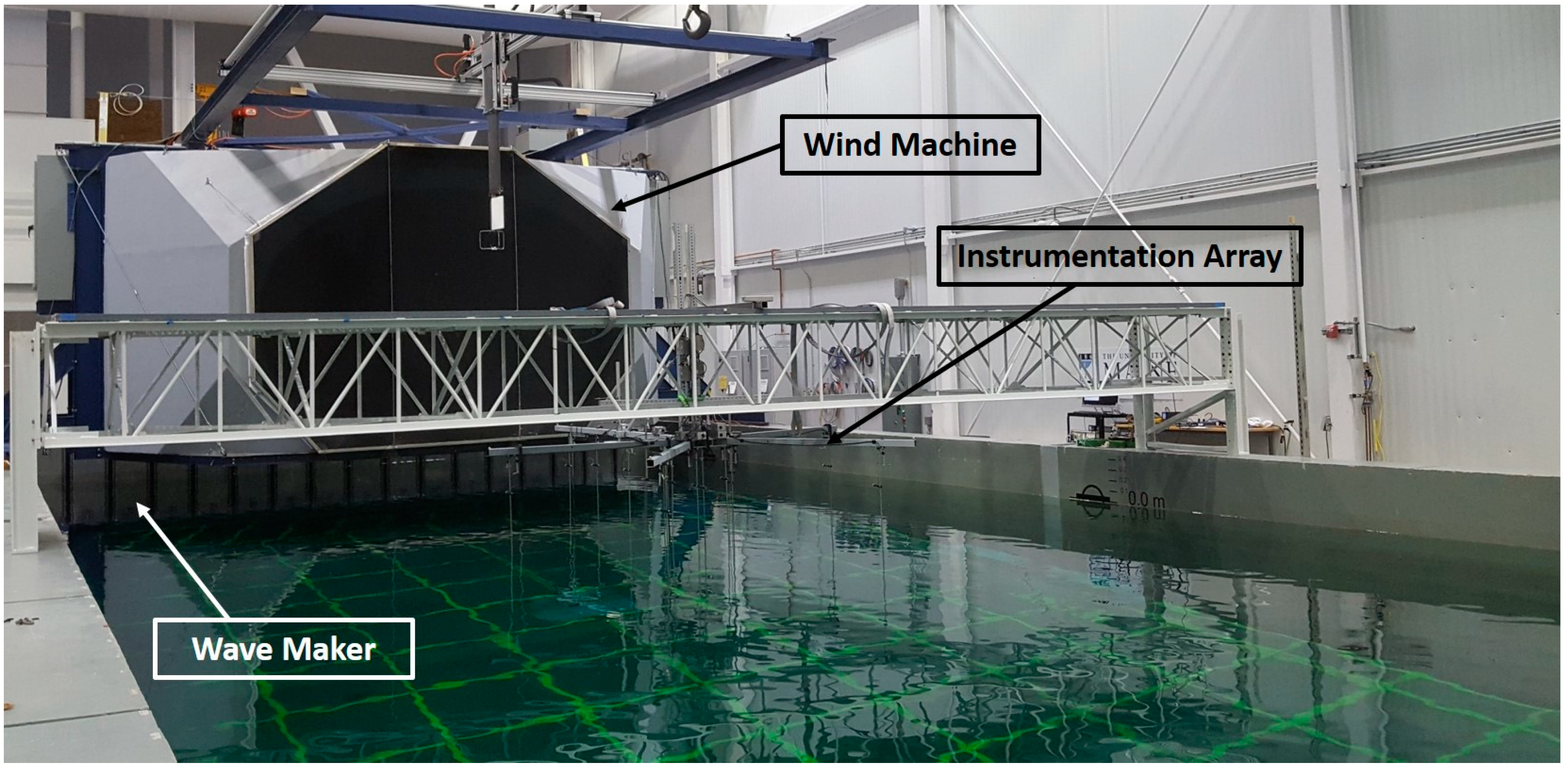
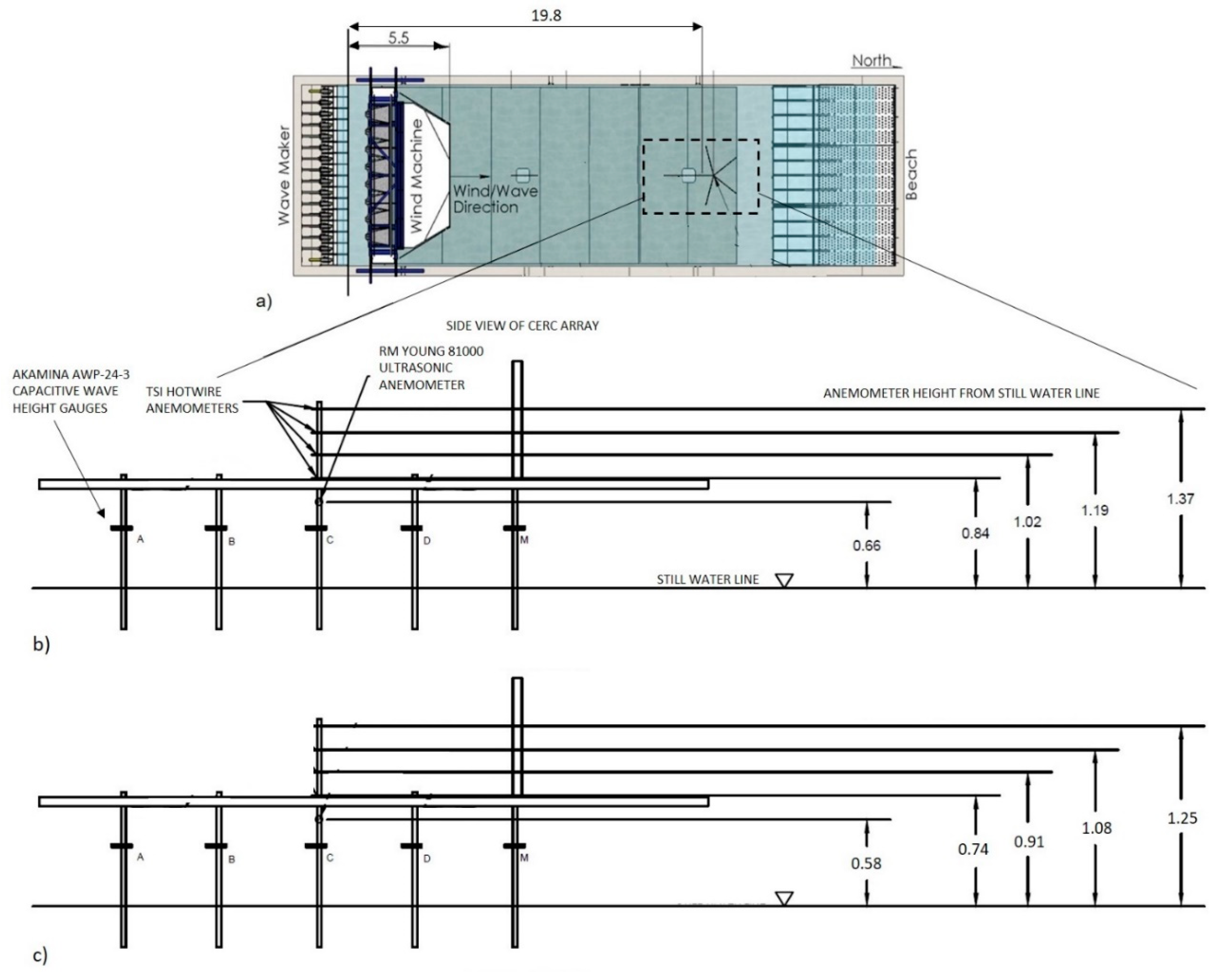
2.1. Test Facility

The laboratory experiments were performed at the Harold Alfond W² (Wind/Wave) Ocean Engineering Laboratory at the University of Maine Advanced Structures and Composites Center (ASCC). The 30 m long by 9 m wide basin has a 16-flap paddle wave generator below a 5 m by 3.5 m by 6 m open-jet wind tunnel (Figure 1). At the opposite end of the basin is an energy-absorbing elliptical beach designed to minimize wave reflection. The basin possesses a moveable concrete floor that was set to allow a water depth of 4.5 m for the duration of the experiment.

2.2. Instrumentation and Data Collection

Two separate data collection campaigns were conducted in the W² in order to obtain a comprehensive data set with a wide range of wave steepness values. A combined total of 15 long wave environments were simulated under five different wind speeds. The first campaign included four test wind speeds: U = 0, 7, 8.5 and 10 m/s and only irregular wave environments. The second campaign expanded the original data set to include more waves of varying steepness and an additional wind speed, U = 5.5 m/s, as well as monochromatic waves. Data were also collected for wind-only seas created in the absence of long waves under each test wind speed, in order to observe the production of wind waves on the water surface.

All wave environments considered in this study are outlined in

Table 1. Wave parameters used to characterize the JONSWAP for the wave environments.

ID	Hs (m)	Tp (s)	aLkL	U (m/s)
1	0.10	2.5	0.032	0, 5.5, 7, 8.5, 10
2	0.15	2.5	0.049	0, 5.5, 7, 8.5, 10
3	0.15	2.5	0.049	0, 7, 8.5, 10
4	0.15	2.25	0.060	0, 5.5, 7, 8.5, 10
5	0.15	2.0	0.076	0, 5.5, 7, 8.5, 10
6	0.25	2.5	0.081	0, 7, 8.5, 10
7	0.15	1.75	0.099	0, 7, 8.5, 10
8	0.35	2.5	0.113	0, 7, 8.5, 10
9	0.30	2.2	0.125	0, 7, 8.5, 10
10	0.40	2.5	0.130	0, 7, 8.5, 10
11	0.27	2.0	0.136	0, 7, 8.5, 10
12M	0.27	2.0	0.136	0, 5.5, 7, 8.5, 10
13M	0.15	2.5	0.049	0, 5.5, 7, 8.5, 10
14M	0.15	1.75	0.099	0, 5.5, 7, 8.5, 10
15M	0.3	1.75	0.197	0, 5.5, 7, 8.5, 10
Wind Only 1	-	-	-	5.5 m/s
Wind Only 2	-	-	-	7 m/s
Wind Only 3	-	-	-	8.5 m/s
Wind Only 4	-	-	-	10 m/s

Symbol M indicates a monochromatic wave.

, including the irregular wave environments, the monochromatic waves (denoted with the symbol M), and wind-only seas. Wave environments are defined by the significant wave height, H_s, and the peak wave period, T_p, the period that corresponds to the frequency at the peak of the wave spectrum. Also presented in Table 1 is the steepness parameter a_Lk_L, where a_L = ½ H_s is the approximate long wave amplitude, and k_L = 2π/L is the long wavenumber where L the wavelength at the peak frequency. A JONSWAP gamma, γ, of 3.3 was used to characterize the frequency spectrum for the irregular waves.

Each of the wave environments presented in Table 1 were coupled with all the wind speeds used during their respective test campaign. In addition to the parameters presented in Table 1 that defined the wave environments, for all irregular environments a cosine 2S shape function was defined, using an S value of 4.0, as well as a directional (angular) spread of ±10 degrees.

The wind and wave environments were examined using a three-dimensional wind/wave array assembled with thirteen wave probes, four hotwire anemometers, and one ultrasonic anemometer (Figure 2). This array was used for both test campaigns with dimensions varying only for the anemometer heights above the water surface, as shown in Figure 2b,c. Wind velocities were collected using four TSI 8455 hotwire anemometers at a sampling rate of 20 Hz with a response frequency of 5 Hz, and one R.M. Young 81000 ultrasonic anemometer sampling at 32 Hz. Surface elevation was measured with 13 Akamina AWP-24-3 capacitive style wave height gauges with accuracy up to 1.35 mm. The wave probes were calibrated and zeroed to a mean water level before the data collection began and were set to sample at a rate of 32 Hz.

The set-up of the wave gauges and anemometers mounted on the instrumentation array are shown in Figure 2b,c for the first and second test campaigns, respectively. The instrumentation array collected surface elevation data and wind speed data at a fetch of 14.31 m with respect to the anemometer staff location (Figure 2a). Data were collected using a directional array assembly similar to the design proposed by the Coastal Engineering Research Center (CERC) [18], but only Probe C, along the center line of the basin was used for post-processing for this study. This is due to its close proximity to the anemometer staff, providing the surface elevation record that most closely corresponds to the reported values of wind speed, air friction velocity and roughness length.

The wave absorbing beach, shown in Figure 2a, is expected to dissipate approximately 90% of the wave energy [19], and the flap wave generators are also designed to actively absorb reflected wave energy. Additionally, a settling time of three minutes was also allotted between wave runs in order to reduce the presence of wave components of the previous test in the next wave record. Each irregular wave environment outlined in Table 1 was run for a 20-min time period. Monochromatic wave environments were run for 15 min.

2.3. Characterizing the Wind Field

Using wind data from both test campaigns, the mean wind speed in the horizontal direction, $\overline{U}$, collected by each anemometer on the staff was used to obtain a profile for U = 7 m/s, U = 8.5 m/s and U = 10 m/s for both campaigns, and additionally, U = 5.5 m/s for the second campaign. These profiles of $\overline{U}$ over the still water surface were used to obtain estimates of $u_{*}$ via a least-squares fit, in a manner similar to Mitsuyasu and Yoshida [20], following the log law,

$$\frac{\overline{U}}{u_{*}}=\frac{1}{\kappa }\ln (\frac{z}{z_0}).$$

(5)

In Equation (5), κ is the von Karman constant (κ ~ 0.4), z is the vertical elevation above the water surface, and $z_0$ is the aerodynamic roughness length [21]. The $u_{*}$ values obtained for the wind speeds, U = 5.5–10 m/s, are on the order of 0.51–0.99 m/s.

Due to the jet-like geometry of the wind machine in the W², the values of roughness length, $z_0$, are on the order of 10⁻² m, which are higher than what is observed in many other laboratories for similar wind speeds. Mitsuyasu and Yoshida [20] obtained values of $z_0$ on the order of 10⁻⁴ m using a similar method of extrapolation of the wind profile via fit to the log law and wind speeds on the order of U = 10 m/s. The values of $z_0$ obtained in the W² are high, and are therefore, more representative of storm sea states observed in the field in which wind waves are more likely to be well developed [22].

3. The Chen and Belcher (2000) Model

The model, presented in Chen and Belcher [5] to estimate the effect of long waves on wind waves, was applied in this study for irregular waves. The CBM model assumes that the momentum associated with the total stress in the wind at the water surface, ${\tau }_{tot}$, is composed of the long wave-induced stress, ${\tau }_L$, and the turbulent wind stress that induces wind wave growth, ${\tau }_t$ so that ${\tau }_{tot}$ = ${\tau }_t+$ ${\tau }_L$ = ${\rho }_a{u}_{*}^2$. The influence of the long wave on wind wave growth is then determined via the reduction of the turbulent wind stress, ${\tau }_t$. This is done considering only four independent parameters: The long wave steepness in the absence of wind, a_Lk_L, the atmospheric pressure coefficient, ${\alpha }_p$, dimensionless frequency, ${\sigma }_{*}$ = ${\sigma }_L{u}_{*}/g$, and dimensionless fetch, $X_{*}$ = $gx/u_{*}^2$, where the subscript, _L, denotes the properties of the long waves in the absence of wind. This is expanded upon in the following sections.

3.1. Long Wave-Induced Stress

The long wave-induced stress, ${\tau }_L$, can be quantified by considering the long wave wind induced growth rate, ${\gamma }_L$, which is defined by

$$\frac{\partial {\mathsf{\Phi }}_L\left(\sigma \right)}{\partial t}={\gamma }_L{\mathsf{\Phi }}_L\left(\sigma \right)$$

(6)

where ${\mathsf{\Phi }}_L$ is the long wave spectral density, and the formulation for ${\gamma }_L$ for monochromatic waves is as expressed in Equation (2). Based on the rate of change of the momentum density of the long wave over time, ${\tau }_L$ is expressed as,

$${\tau }_L={\rho }_w{{\displaystyle \int }}_0^{\infty }{\gamma }_L{\sigma }_L{\mathsf{\Phi }}_L\left(\sigma \right)d\sigma$$

(7)

Therefore, if ${\tau }_L$ is quantified for long waves in the absence of wind and $u_{*}$ is known, ${\tau }_t$ can be calculated as ${\tau }_t={\tau }_{tot}$ − ${\tau }_L$. In order to accurately quantify the long wave-induced stress, the growth of the long wave, ${\gamma }_L$, as expressed in Equation (2) must be quantified.

3.2. Growth Rate of the Long Wave, ${\gamma }_L$

Belcher [15] investigated non-separated sheltering induced wave growth and van Duin [16] investigated wave growth induced by turbulent air flow over waves. Both studies arrived at similar formulations of the wave growth rate due to these mechanisms (Equation (2)), after making several important assumptions. The first major assumption is that the wave steepness is on the order of ak << 1. The second major assumption is that the long waves fall within the regime of slow waves or fast waves which are defined by the wave age thresholds of $c/u_{*}$ < 15 and $c/u_{*}$ > 25, respectively, for $k{z}_0$ ~ 10⁻⁴. Finally, the model of Belcher [15] was formulated based on the energy equation for deep water waves; therefore, Equation (2) can only be applied to waves that can be considered short, based on their relative depth, d/L, where d is the water depth, and L is the wavelength. The origin of the growth rate coefficient, β, is an integral parameter in the CBM, which describes the growth of waves by the wind. This parameter, first presented in Equation (2), has evolved over decades through consideration of different mechanisms by which it is possible for the wind to transfer energy and momentum to the waves [15,23,24]. The development of β used in the CBM is based on the physical model by Belcher [15] of non-separated airflow sheltering over slow waves, which are defined by [25] as waves for which,

$$k{z}_c=k{z}_0{e}^{\kappa c/u_{*}}\ll 1,$$

(8)

where $z_c$ is the critical layer height. For slow waves, for which the wind speed is greater than the wave speed, the critical layer is small, and therefore, $k{z}_c$ is small, indicating that the waves are forced by wind and not vice versa [25].

The model presented in Belcher [15] to quantify β is based on the criterion that the waves fall within this slow wave regime, indicating that there is non-separated sheltering immediately above the water surface. Although the values of $z_0$, on the order of 0.01 m, obtained in the W² are high compared to other laboratory wind fields [20] for similar wind speeds, the values of $k{z}_c$ for the highest wind speed, U = 10 m/s, are on the order of 10⁻¹ m. This indicates that the wave environments of this study fall within the slow wave regime.

The non-separated sheltering assumption guarantees the existence of an inner layer (just above the water surface) and a middle layer (above the inner layer) that are characterized by different flow behaviors, yet do not experience boundary layer separation at the wave crests. In order to calculate an appropriate value of β to use for the model for the irregular waves, the inner layer, l_i, and middle layer, h_m, heights were calculated following the methodology of [24] using the long wave data under the action of wind. To iteratively quantify these length scales, the assumption was made that both l_i and h_m were greater than $z_c$ (equal to the matched height, $z_m$, as defined by [24]) to be the vertical location at which the wind speed and the wave speed are equivalent.

To calculate the β, five components must be considered [15],

$$\beta ={\beta }_{s{z}_i}+{\beta }_{s{u}_i}+{\beta }_{p_o}+{\beta }_{{\eta }_s}+{\beta }_{u_s}$$

(9)

The first two of the five components account for non-separated sheltering effects, including the influence of shear stress on the inner region due to undulations on the water surface, ${\beta }_{s{z}_i}$, and due to changes of velocity at the water surface, ${\beta }_{s{u}_i}$. The third is due to the variations in pressure in the outer region, ${\beta }_{p_o}$. The respective equations are,

$${\beta }_{s{z}_i}=2{(\frac{{\overline{U}}_{ml}-c}{{\overline{U}}_{il}-c})}^4\{2-\frac{c}{{\overline{U}}_{il}}\}$$

(10)

$${\beta }_{s{u}_i}=-2{(\frac{{\overline{U}}_{ml}-c}{{\overline{U}}_{il}-c})}^2 \frac{c}{{\overline{U}}_{il}}$$

(11)

$${\beta }_{p_o}=2\kappa {\delta }^{2n}\{\frac{{\overline{U}}_{ml}-c}{u_{*}}\}$$

(12)

where ${\overline{U}}_{ml}$ and ${\overline{U}}_{il}$ are the mean wind speeds at h_m and l_i, respectively, calculated as,

$${\overline{U}}_l\left(z\right)=(\frac{u_{*}}{\kappa })\ln (\frac{z}{z_0})$$

(13)

where z is set equal to h_m and l_i, and the subscript l is set to ml or il, respectively. In Equation (12), $\delta =\kappa /\left|ln\left(k{z}_c\right)\right|$ for slow waves [25] and n is a model coefficient between 0 and 1 [15], set here to 0.5. The fourth and fifth terms in Equation (9) arise from the wave-induced surface shear stress, where the first contribution is from the waves, ${\beta }_{{\eta }_s}$, and the second from variations in surface velocity, ${\beta }_{u_s}$, where

$${\beta }_{{\eta }_s}=\frac{2{({\overline{U}}_{ml}-c)}^2}{({\overline{U}}_{il}-c){\overline{U}}_{il}}$$

(14)

$${\beta }_{u_s}=-\frac{2c}{{\overline{U}}_{il}}$$

(15)

According to Belcher [15], the term ${\beta }_{s{z}_i}$ should dominate the growth rate coefficient for slow waves, which is what is expected for this study. Once β has been quantified, ${\gamma }_L$ can be determined and used for calculation of the long wave-induced stress, ${\tau }_L$ (Equation (7)). Combining Equation (2) and Equation (7), an expression for the dependence of the long wave amplitude development with fetch (under a steady wind), denoted, ${ϵ}_L$, is formulated as

$${ϵ}_L=exp\left[2\frac{{\rho }_a}{{\rho }_w}\frac{{\alpha }_p}{1+\frac{1}{2}{(a_L{k}_L)}^2{\alpha }_p{ϵ}_L}{\sigma }_{*}^4\left(X_{*}-X_{0*}\right)\right]$$

(16)

where the subscript, ₀, denotes a value measured at the location of the initial fetch, meaning the horizontal distance at which the wind first impacts the long wave. The result from combining Equations (7) and (16) is a ratio which describes the distribution of the turbulent stress to the total stress,

$$\frac{{\tau }_t}{{\tau }_{tot}}=\frac{1}{1+\frac{1}{2}{(a_L{k}_L)}^2{\alpha }_p{ϵ}_L}$$

(17)

To assess the influence of the long waves on the wind waves through the reduction of the turbulent stress, the CBM utilizes the ratio of the wind wave energy in the presence of long waves, $E_{L+ww}$, to the wind wave energy in the absence of long waves, $E_{ww}$, to compare the model results to data collected in the laboratory. Assuming that in the presence of the long wave $u_{*}$ can be rewritten in terms of the turbulent stress as $u_{*}={({\tau }_t/{\rho }_a)}^{1/2}$, the ratio $\frac{E_{L+ww}}{E_{ww}}$ is derived from Equation (4) as,

$$\frac{E_{L+ww}}{E_{ww}}={(\frac{{\tau }_t}{{\tau }_{tot}})}^{1.36}$$

(18)

which, for short fetch distances, such as the conditions in the laboratory, can be simplified to

$$\frac{E_{L+ww}}{E_{ww}}={(\frac{1}{1+\frac{1}{2}{(a_L{k}_L)}^2{\alpha }_p})}^{1.36}$$

(19)

due to the dependence of Equation (19) on $a_L{k}_L$ and ${\alpha }_p.$ The energy ratios presented from the model (Equations (18) and (19)) will be compared to estimates made directly from laboratory data. Data analysis techniques used to determine the ratio from data will be described in the following section. For further details on the model derivation, the reader is referred to Chen and Belcher [5].

4. Methods: Data Analysis

4.1. Experimental Energy Ratio, $\frac{E_{L+ww}}{E_{ww}}$

This section describes the data analysis performed in order to obtain experimental values of $\frac{E_{L+ww}}{E_{ww}}$ directly from the laboratory data to compare to the values of $\frac{E_{L+ww}}{E_{ww}}$ obtained from the model. The procedure for obtaining the values of $E_{ww}$ and $E_{L+ww}$ will be discussed separately, as additional data analysis techniques were required to obtain $E_{L+ww}$ due to the presence of the long wave in the surface elevation records.

To calculate $E_{ww}$ directly from the data, a spectral analysis and a wavelet analysis were performed on the surface elevation records collected at Probe C for wind only runs for all wind speeds. Using the wave gauge sampling interval of 0.0313 s, a Fast Fourier transform (FFT) of 1024 points was applied to the surface elevation record with the first two minutes of the record removed as a contribution to start-up time for the wind waves to develop fully. Frequencies lower than 0.1 Hz were cut-off in order to accurately quantify the peak period from the spectra, and a high pass filter with a cut-off at f = 2 Hz was applied to remove residual low frequency energy observed in the wave spectra. The variance of the wind sea, $\overline{{\eta }^2}$ was quantified from the spectral results as $\overline{{\eta }^2}$ = $S_f\Delta f$, where $S_f$ is the spectral energy at each frequency separated by Δf = 0.0078 Hz. The energy of the wind sea alone was then quantified as $E_{ww}={\rho }_{w}g\overline{{\eta }^2}$.

To calculate $E_{L+ww}$ from the data, a wavelet reconstruction method, outlined in Torrence and Compo [26] was applied. First, a wavelet transform was performed on the data in order to analyze the energy within the high frequencies and how it varies with time. The Morlet mother wavelet function was used with a spacing of 0.01 between discrete scales to provide a fine resolution. All other input parameters were set to default [26]. The sampling interval, in this case, was the same as the sampling interval of the surface elevation record, which was approximately 0.0313 s. Surface elevation records used in the analysis were unfiltered in order to capture the high frequency oscillations associated with wind waves. Based on the observed peak frequencies of the wind sea alone and the results of the wavelet analysis, the energy associated with frequencies, f > 2 Hz, were deemed to be associated predominantly with energy input from the wind. Therefore, the wavelet reconstruction was used to recreate the surface elevation records for each case using only the energy associated with f > 2 Hz.

Following the reconstruction of the surface elevation record of the high frequencies for the irregular waves, despiking of each individual record was performed, using a threshold wind wave amplitude of 1 cm to identify spikes, and replacing the spikes with the mean wave amplitude of the record, which is one option for spike replacement as suggested by Goring and Nikora [27]. Prior to obtaining the variance of each high frequency record for the irregular and monochromatic waves, a second method to ensure removal of any potentially remaining low frequency long wave energy was applied, which consisted of a high-pass filter with a cut-off frequency of f = 2 Hz.

Following the high-pass filter, the spectral analysis was performed on the high frequency record and the energy of the wind waves in the presence of the long wave, $E_{L+ww}$, was calculated using the same methods as described to calculate $E_{ww}$. For the mixed sea states of monochromatic waves and wind, the code WaveSpectraFun from the OCEANLYZ Ocean Wave Analyzing Toolbox was used to perform the spectral analysis on the high frequency records [28]. From the spectral analysis of the monochromatic waves, the same method was then used to quantify $E_{L+ww}$ as outlined for the irregular waves, despite the smaller spread of the peak spectral energy. This was performed for consistency and was decided based on the knowledge of the distribution of spectral energy for the wind sea alone.

4.2. Quantifying the Growth Rate Coefficient and the Atmospheric Pressure Coefficient

Data from several laboratory studies [1,2,3] are used to validate the CBM in Chen and Belcher [5]. Values of ${\alpha }_p$ = 80 and ${\alpha }_p$ = 160 were selected based on a fit to the data, and values of β were quantified from the relation,

$$\beta =\frac{{\alpha }_p}{1+k_L^2\overline{{\eta }_L^2}{\alpha }_p},$$

(20)

from Chen and Belcher [5]. The values of β obtained via this method were considered acceptable because they fell within the range of β = 34 ± 16, which was the range obtained by Plant [23]. This practice was adopted here in the selection of an appropriate ${\alpha }_p$ value for the wave data of this study. A ${\alpha }_p$ value was selected based on fit of the model results to the experimental energy ratios, then β was quantified via Equation (20) and verified to be within the range of values obtained by Plant [23].

5. Results

5.1. CBM Results for the Monochromatic Waves

As was found in Chen and Belcher [5], the monochromatic waves in this study indicate that as wave steepness increases, energy is transferred from the wind waves to the long waves, ultimately decreasing the energy ratio. This was observed for all wind speeds considered in this study, except U = 5.5 m/s (Figure 3). The model results in Figure 3 are presented both as the model prediction curve (red line), using the short fetch approximation of Equation (19), and as model points (red, open symbols), calculated specifically for each wave environment using Equations (17) and (18), which differ only from the model curve due to their dependence on ${ϵ}_L$, which for short fetch, such as that in a laboratory, is approximately 1 [5]. The experimental results deviate from the model at U = 5.5 m/s due to reduced wind wave growth leading to a lower steepness threshold for wind wave suppression. The model does well to predict the energy ratio for U = 5.5 m/s up until a value of a_Lk_L ~ 0.12–0.14 is achieved.

For the model (Equation (19)), ${\alpha }_p$ was set to 100 based on best fit to the data and were compared to values of ${\alpha }_p$ used to assess previous experimental data [1,2] in Chen and Belcher [5], for which ${\alpha }_p$ ~ 80–160.

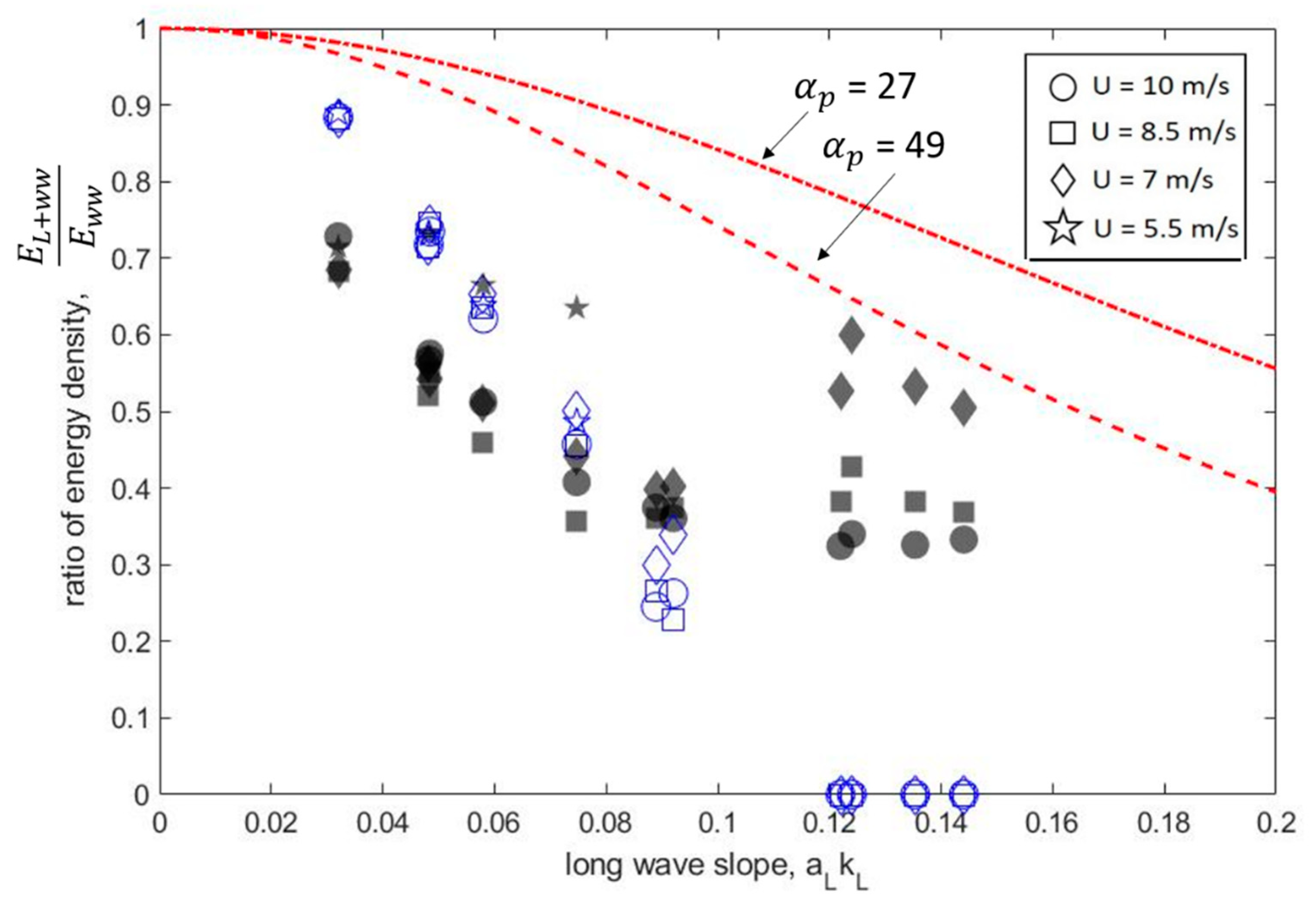
5.2. CBM Results for Irregular Waves

Here the CBM is applied to the irregular waves of this study, and it is shown that the decrease in the energy ratio with increasing steepness occurs far more quickly than is predicted by the CBM (Figure 4). Using the same value of ${\alpha }_p$ = 100 as was used in the model for the monochromatic waves, the model results were computed for the irregular waves. In order to apply Equation (2) and Equation (17) to the irregular wave environments, the values of c_L, k_L and ${\sigma }_L$ are based on the significant properties of the waves, as opposed to the single frequency of a monochromatic wave. Here, the dispersion relation was used to iteratively quantify L based on the peak period, T_p, of the wave spectrum, c_L was calculated as c_L = L/T_p, k_L as k_L = 2$\pi /L$, and ${\sigma }_L$ as ${\sigma }_L$ = 2$\pi$f_p, where f_p is the peak frequency of the wave spectrum. The variance of the long wave, $\overline{{\eta }_L^2}$, was quantified as the zeroth-moment of the wave spectrum.

The results in Figure 4 show that the slope of the model curve, calculated from Equation (19), and the model points, computed from Equation (17) in Equation (18), is too small to fit the trend of the experimental energy ratios with increasing steepness for the irregular waves. It was estimated that an ${\alpha }_p$ of approximately 300 would be required in order to fit the model results to the experimental energy ratios of the irregular waves (not shown), which, for the range of steepness values considered (a_Lk_L ~ 0.03–0.15) produces corresponding β values between 69–264. The value of ${\alpha }_p$ and the corresponding values of β are far too large to be reasonable, falling outside the range obtained by Plant [23].

The waves with a_Lk_L > 0.1 do not follow the model curve, nor the trend of the model energy ratios, due to breaking of the tallest waves, which induces high frequency energy [29] that results in an increase in the variance of the high frequency record. Wave breaking of the significant waves of these cases was confirmed visually in a test video of the experiment (not shown). Because the value of ${\alpha }_p$ required to fit the model to the experimental data is far too large to be reasonable, it was necessary to directly quantify values οf β and the associated ${\alpha }_p$ for the irregular waves following Belcher [15] and Belcher [24], as outlined in Section 3.2 rather than using ${\alpha }_p$ as a fitting parameter. These results will be presented next.

5.3. The Growth Rate Coefficient and Atmospheric Pressure Coefficient for the Irregular Waves

Following the methodology of Belcher [15] summarized in Section 3.2, values of β were quantified using Equations (10)–(12), (14) and (15) based on the irregular wave data collected in the experiments. It was first verified that the assumptions of the model by Belcher [15] were met for the wave environments of this study; the long wave environments fall within the slow wave regime, i.e., $c/u_{*}$< 15, are of steepness, ak << 1, and can be considered deep water, i.e., a relative depth, d/L of approximately 0.5 or greater. The long wave data in the absence of wind were then used to obtain the properties of the waves to convert the actual values of β to ${\alpha }_p$ through the iterative calculation of Equation (20). For the irregular waves of this study, under U = 5.5–10 m/s, ${\alpha }_p$~ 27–49, and β ~ 25–34. Figure 5 shows the estimates of β versus wave age, $c/u_{*},$ for the irregular long waves of this study. The values of β obtained for the irregular waves fall within the range outlined by Chen and Belcher [5] based on values determined by Plant [23] of approximately β = 34 ± 16. The corresponding values of ${\alpha }_p$ for the irregular long waves versus $c/u_{*}$ are shown in Figure 6.

The values of ${\alpha }_p$ for the irregular waves of this study are low compared to the values used for fit to the laboratory data obtained by Mitsuyasu [1] (${\alpha }_p$ = 80) and Phillips and Banner [2] (${\alpha }_p$ = 160), and are therefore, more representative of ocean conditions as opposed to the conditions in the laboratory. Chen and Belcher [5] suggest that in the ocean, β is small, and because of the small slopes associated with ocean swell, imply that ${\alpha }_p$ ≈ β. The waves of this study are not representative of ocean swell, as discussed in Section 1, but are more representative of long wind waves which are typically steeper than ocean swell [30]. The wind field conditions simulated in the W², however, are more similar to ocean conditions during storm seas, as discussed in Section 2.3, due to large roughness values of $z_0$ ~ 10⁻² m. These results for ${\alpha }_p$ and β suggest that the conditions of this study are representative of long waves coupled with strong wind fields (U ~ 7–10 m/s) in the ocean.

The results for the application of the CBM model to the monochromatic and irregular wave data of this study have been presented, as well as values of β associated with the conditions of the wind field and the irregular wave environments. It was found that the model was able to accurately predict the reduction of wave energy with increasing steepness in the monochromatic wave environments, but not the irregular wave environments. In the latter case, using the atmospheric pressure coefficient (${\alpha }_p$) and growth rate coefficient (β) as fit parameters, the model underestimates the reduction in the energy of the wind waves with increasing long wave steepness. Unrealistic values of ${\alpha }_p$ and β are required to capture this trend. Implications of these results will be discussed next, and a modified version of the CBM model will be presented that adapts the original model for use with irregular wave environments using the values of β that were directly quantified.

6. Discussion

The goal of this study is to determine if the CBM for wind wave suppression on the surface of long waves is applicable to irregular waves. In order to reach this goal, two specific research questions were defined: (1) Does the CBM accurately predict the decrease in the energy of the wind waves in the presence of irregular waves of increasing steepness? (2) Can the CBM model be improved by accounting for the long wave energy at each frequency of the wave spectrum for an irregular wave environment? The CBM model was first applied here to monochromatic waves of this study to validate it for the wave environments simulated in the W² (Wind/Wave) Basin and the results show that it does well to predict the variation in the experimental energy ratio with increasing long wave steepness for these waves. To address research question 1, the CBM was then applied to the irregular wave environments simulated in the W². The model results for the irregular waves underpredict the slope of the experimental energy ratios with increasing long wave steepness, and therefore, do not accurately predict the decrease in the energy of the wind waves in the presence of the irregular long waves of increasing steepness. An unreasonably high value of ${\alpha }_p$ (~300) is required for use in the model in order to fit the model results to the experimental energy ratios, which for the range of steepness values considered ($a_L{k}_L$ ~ 0.03–0.15) produce corresponding β values between 69–264. For slow waves, $c/u_{*}$ < 15, which is the regime within which the waves of this study fall, these β values are much higher than values observed in both laboratory and ocean environments [5,8,23]. Belcher [15] concluded that for slow waves, β ≈ 20.

The reason for the discrepancy in the model’s applicability to monochromatic and irregular waves, is that the model is formulated to account for only the momentum of the long wave at a singular frequency, ${\sigma }_L$. This is shown, namely, in Equation (7), where ${\tau }_L$ is based on the rate of change of momentum of the long wave at ${\sigma }_L$. While this formulation is accurate for monochromatic waves, whose wave energy exists at a single frequency, it is inapplicable to irregular wave environments due to the spread of wave energy over a range of frequencies. Therefore, direct application of the CBM to irregular long waves underestimates the rate of change of $\frac{E_{L+ww}}{E_{ww}}$ with increasing a_Lk_L, resulting in an overestimation of ${\alpha }_p$. In order to apply the model to irregular waves, the long waves must be treated as a superposition of monochromatic waves that occur at a wide range of frequencies. A modified version of the CBM model that invokes this principle is introduced next.

6.1. Modifying the CBM for Irregular Long Waves

In order to modify the CBM for the application to irregular long waves, Equation (7) must be modified to account for the momentum associated with each wave frequency in the wave spectrum. The modified expression for ${\tau }_L$ for irregular waves becomes

$${\tau }_L={\rho }_w{{\displaystyle \int }}_0^N\left[{\gamma }_{L1}{\sigma }_{L1}{\mathsf{\Phi }}_{L1}\left(\sigma \right)+{\gamma }_{L2}{\sigma }_{L2}{\mathsf{\Phi }}_{L2}\left(\sigma \right)+\dots {\gamma }_{LN}{\sigma }_{LN}{\mathsf{\Phi }}_{LN}\left(\sigma \right)\right]d\sigma$$

(21)

where the integration is performed over the range of frequencies of the wave spectrum. To calculate this expression, the wavelet reconstruction method described by Torrence and Compo [26] was used. The reconstruction method allows the original surface elevation record, η_L, to be broken down into individual records, η_Lj, based on the energy contained within each discrete frequency scale, j, where j = 1, 2, …, N, and N is the number of scales of the wavelet, and ${\sigma }_{Lj}$ is the frequency associated with each scale. The terms within the bracket of Equation (21) were quantified for each scale of the wavelet, j, which are separated by a spacing, dj = 0.1. For each η_Lj, γ_Lj was calculated by quantifying c_Lj for the waves of the record of scale j. The $u_{*}$ associated with each wind speed was used, and the ${\sigma }_{Lj}$ value is quantified as the inverse of the Fourier period, T_j, times 2π. The value of β used in Equation (2) to calculate γ_Lj for each wave environment was the calculated value of β based on the properties of the entire long wave surface elevation record. To quantify ${\mathsf{\Phi }}_L$, the power at each scale was integrated over time, in order to provide an estimate of ${\mathsf{\Phi }}_{Lj}$ for each ${\sigma }_{Lj}$.

The results of the modified CBM described above, which accounts for the energy associated with a range of frequencies of the wave spectrum, show better agreement with the trend of the experimental energy ratios with increasing wave steepness for the irregular waves for a_Lk_L = 0.03−0.09 (Figure 7). Moreover, shown in Figure 7 are the model curves generated by the original CBM using the values of β (and, thus, ${\alpha }_P$) quantified directly from Equations (10)–(12), (14) and (15). The model curves shown in the figure correspond to the maximum and minimum ${\alpha }_P$ values obtained for the irregular waves. Physically, the maximum and minimum ${\alpha }_P$ values represent the model’s prediction for the longest (in terms of wavelength) and shortest waves in the irregular data set, respectively. Despite the direct quantification of β and ${\alpha }_P$, the model continues to under predict the slope of the trend in the experimental energy ratios. The original CBM results are shown in order to emphasize the improvement of the results of the modified model using the same values of β.

It is important to note that the modified CBM provides results based on a measured wave spectrum, and due to the need to consider the multiple wave frequencies of an irregular spectrum, the equation that was used in the CBM (Equation (17)) to predict wind wave suppression as a function of long wave steepness is inapplicable. The derivation of Equation (17) in Chen and Belcher [5] is based on the use of Equation (2), for which the growth rate is a function of a single wave frequency, and therefore, fails for irregular waves for which energy exists at multiple frequencies. The modified CBM described in this section, therefore, cannot be used as a prediction tool for estimating wind wave suppression based on a_Lk_L and ${\alpha }_P$ alone, and instead relies on the availability of an observed wave spectrum from which ${\tau }_L$ (Equation (21)) can be quantified.

For the updated model, the values of $\frac{E_{L+ww}}{E_{ww}}$ are set to 0 when ${\tau }_L$ > ${\tau }_{tot}$, because based on the momentum equation, ${\tau }_t={\tau }_{tot}-{\tau }_L$, a value of ${\tau }_L$ > ${\tau }_{tot}$ gives a negative estimate of ${\tau }_t$, which makes the value of $\frac{E_{L+ww}}{E_{ww}}$ based on Equation (19) complex. Physically, ${\tau }_t$ cannot be negative because as the horizontal momentum associated with the wave-induced stress, ${\tau }_L$, increases, the portion of the total momentum associated with ${\tau }_t$ decreases if ${\tau }_{tot}$ is constant [5], which prevails in the reduction of available momentum to grow the wind waves. If ${\tau }_L={\tau }_{tot}$, the total momentum from the wind is absorbed by the long wave and ${\tau }_t$ is completely reduced to 0, at which point the wind waves are completely suppressed by the long wave.

The modified model results are slightly overpredicted for waves of low steepness (a_Lk_L ~ 0.03–0.06). This is likely due to the estimates of $u_{*}$ used in the model. The estimates of $u_{*}$ were obtained via a log law fit to the wind profile measurements collected in the absence of the waves at a distance z = 0.20–1.40 m above the water surface, as described in Section 2.3. The estimates of $u_{*}$ may be slightly underpredicted due to the lack of proximity of the wind measurements to the water surface and the use of a log law fit to a wind profile that is more similar to a jet. In the modified model, the equation, ${\tau }_t={\tau }_{tot}-{\tau }_L$, where ${\tau }_{tot}={\rho }_a{u}_{*}^2$, is used to quantify ${\tau }_t$ from the values of ${\tau }_L$ calculated using the new model equation (Equation (21)). Using estimates of $u_{*}$ obtained from the extrapolated wind profile, ${\tau }_{tot}$ may be slightly underpredicted. This could result in the underprediction of ${\tau }_{tot}$, which would, thus, overpredict the model energy ratio, $\frac{E_{L+ww}}{E_{ww}}={(\frac{{\tau }_t}{{\tau }_{tot}})}^{1.36}$. For waves of higher steepness, a_Lk_L > 0.06–0.09, the model is more accurate, which is likely because $u_{*}$ is reduced in the presence of steep waves due to the obstruction of the wind profile by the wave profile; thus, the experimental results conform better to the modified model results using the estimated values of $u_{*}$ from a log law approximation.

The modified model does well to describe the decrease in $\frac{E_{L+ww}}{E_{ww}}$ for the high wind speeds (U = 7, 8.5, 10 m/s) until a_Lk_L ≥ 0.1. To provide some explanation for this threshold, the modified model results, which are based on the measured $u_{*}$ and calculated β values for each wind speed, ${\tau }_t$ and ${\tau }_L$ are investigated in relation to steepness, a_Lk_L (Figure 8). The a_Lk_L at which ${\tau }_t$ and ${\tau }_L$ are nearly equal is approximately 0.075, but this threshold increases slightly with increasing wind speed. Until the steepness of the long wave environment is greater than approximately 0.075, ${\tau }_t$, which is responsible for wind wave growth on the long waves, is the dominant fraction of the total surface stress. Once this transitional a_Lk_L value is reached, the long wave is steep enough to begin to receive the majority of the wind energy input, reducing the available ${\tau }_t$ for wind wave growth, which results in the suppression of the wind waves. For steepness values above 0.075, the model is no longer predicting the transfer of wind energy to the long wave, but rather the suppression of the wind waves by the long waves, and therefore, breaks down.

It has been shown that by modifying the CBM model to incorporate the growth of individual wave components and directly quantified values of β, it can be used to describe the trend in the experimental energy ratios with increasing steepness for irregular waves. For the application of the modified CBM presented here to irregular waves, it is essential that β be quantified directly following the methodology of Belcher [15,24] using Equations (10)–(12), (14) and (15). A corresponding value of ${\alpha }_p$ must then be calculated using Equation (20), as it has been shown in Figure 7 that use of ${\alpha }_p$ as a fitting parameter is inadequate. Additionally, to ensure that the calculated values of β are appropriate, it is important to determine if they fall within the range of values observed for field conditions by Plant [23] (β = 34 $\pm$ 16) prior to use of the corresponding ${\alpha }_p$ values in the model. To physically understand the mechanisms contributing to the growth of the long wave, the individual contributions to β will be discussed next.

6.2. Analysis of the Growth Rate Coefficient

As discussed in Section 3.2, there are five physical mechanisms that contribute to β and ultimately cause the waves to grow. As noted by Belcher [15], for the slow wave regime, i.e., $c/u_{*}$< 15, it is the contribution from the shear stress on the inner region due to undulations on the water surface associated with non-separated sheltering, ${\beta }_{s{z}_i}$, that will dominate the growth of the long waves under wind action. This claim is supported by the calculated components of β for the irregular long waves of this study (Figure 9). In fact, the contribution from ${\beta }_{s{z}_i}$ is nearly ten times larger than the contribution from the wave-induced surface stress component, ${\beta }_{{\eta }_s}$, which is believed to be the largest contributor to wave growth in the fast wave regime. i.e., $c/u_{*}$ > 25 [15].

The contribution from the varying surface velocity associated with the non-separated sheltering, ${\beta }_{s{u}_i}$, is negative because it accounts for a decrease in the pressure at the surface due to negative wave-induced stress over the inner region. This negative portion of the wave-induced stress is caused by the orbital motions of the waves [15]. The contribution from the varying surface velocity associated with the surface stress, ${\beta }_{u_s}$, is also negative, but for slow waves, this contribution to the growth coefficient is typically small, on the order of 1 [25]. The terms ${\beta }_{s{u}_i}$ and ${\beta }_{u_s}$, therefore, counteract the contributions from the other terms, nearly cancelling the contributions from ${\beta }_{{\eta }_s}$ and the contribution from changes in pressure in the inner region associated with non-separated sheltering, ${\beta }_{p_o}$.

This study has investigated the mechanisms that contribute to the growth of the long wave by analyzing the contributions to β. A research question that has been posed by many studies, but remains unanswered is, what physical mechanism is responsible for the suppression of wind waves on the surface of long waves? Although this study cannot draw conclusions that answer this question, it does support the conclusion drawn by Chen and Belcher [5] that the momentum available to grow the wind waves is dependent on the amount of momentum absorbed by the long waves due to direct coupling between the long waves and the wind. This suggests that the suppression of the wind waves is a result of reduced turbulent stress, which is proportional to the long wave-induced stress which increases with increasing a_Lk_L. Additionally, Chen and Belcher [5] mention that, for the application of the model (Equation (18)), the fetch law presented in Equation (4), from which Equation (18) is derived, must be replaced with a fetch law obtained from observational measurements in the ocean. To investigate the applicability of the modified model to open ocean conditions, the energy ratio was also derived from fetch laws presented in Komen et al. [31] for open ocean sea states and produced results with a negligible difference to Equation (18) (not shown). The agreement between the energy ratio of Equation (18) derived by Chen and Belcher [5] and that derived from the fetch laws for open ocean conditions is contributed to the wind fields generated by the wind machine in the W² Basin, which compares well to measured conditions in the ocean [22].

7. Conclusions

The Chen and Belcher [5] wind wave suppression model was applied to a comprehensive data set of long monochromatic and irregular waves of varying properties (H_s and T_p). The goal of this study is to investigate the use of the CBM for wind wave suppression on the surface of irregular waves. The model accurately predicts the variation in the energy ratio, $\frac{E_{L+ww}}{E_{ww}}$, with increasing wave steepness, a_Lk_L, for monochromatic waves under wind speeds varying from U = 7–10 m/s, which contain wave energy at only a single frequency. When applied to the irregular wave environments, unreasonably large estimates of ${\alpha }_p$ are required to fit the CBM results to the trend of the experimental energy ratios with increasing a_Lk_L, and therefore, it cannot be directly applied to irregular waves. The CBM was modified for the application to irregular waves by considering a wide range of frequencies in the expression for the long wave-induced stress, as opposed to a single frequency consistent with monochromatic waves, in order to account for the growth of the individual wave components of an irregular sea state. When this modification is considered, the CBM model is able to better describe the trend in $\frac{E_{L+ww}}{E_{ww}}$ with a_Lk_L well using the directly quantified values of the atmospheric pressure coefficient (${\alpha }_p$ ~ 25–50), however, the derivation used in the CBM to arrive at Equation (17) becomes invalid due to the consideration of multiple wave frequencies. Because of the failure of Equation (17) to be applicable for irregular waves, the modified CBM is not a prediction tool, but instead allows for an estimate of the energy ratio under varying wind by use of a single wave spectrum in the absence of wind and characteristic values of β and $u_{*}$ for the conditions of interest.

This study further validates the CBM model for monochromatic waves in wind environments of elevated roughness $z_0$ ($z_0$ ~ 10⁻² m), and suggests a correction to the model to make it more applicable to realistic sea states that are better represented by irregular waves. Future work should include the investigation of a method to infer a prediction tool from the newly proposed long wave-induced stress formulation (Equation (21)) to allow for the prediction of wind wave suppression as a function of the long wave steepness for irregular waves directly. Application of this modified model to field conditions or to irregular waves simulated in a laboratory of longer fetch could help to further validate this model and refine the conditions for which it is applicable. Given more observational data, improved thresholds, in terms of long wave steepness and wind speed, could be determined and used in the wave models to identify sea states that are susceptible to the suppression of wind waves.

References

1. Mitsuyasu, H. Interactions between water waves and wind (I). Rep. Res. Inst. Appl. Mech. Kyushu Univ. 1966, 14, 67–88. [Google Scholar]
2. Phillips, O.M.; Banner, M.L. Wave breaking in the presence of wind drift and swell. J. Fluid Mech. 1974, 66, 625–640. [Google Scholar] [CrossRef]
3. Donelan, M.A. The Effect of Swell on the Growth of Wind Waves. J. Hopkins APL Tech. Dig. 1987, 8, 18–23. [Google Scholar]
4. Makin, V.K.; Branger, H.; Peirson, W.L.; Giovanangeli, J.P. Stress above Wind-Plus-Paddle Waves: Modeling of a Laboratory Experiment. J. Phys. Oceanogr. 2007, 37, 2824–2837. [Google Scholar] [CrossRef]
5. Chen, G.; Belcher, S.E. Effects of Long Waves on Wind-Generated Waves. J. Phys. Oceanogr. 2000, 30, 2246–2256. [Google Scholar] [CrossRef]
6. Ardhuin, F.; Rogers, E.; Babanin, A.V.; Filipot, J.; Magne, R.; Roland, A.; Westhuysen, A.V.D.; Queffeulou, P.; Lefevre, J.; Aouf, L.; et al. Semiempirical Dissipation Source Functions for Ocean Waves. Part I: Definition, Calibration, and Validation. J. Phys. Oceanogr. 2010, 40, 1917–1941. [Google Scholar] [CrossRef] [Green Version]
7. The WAVEWATCH® Development Group (WW3DG). User Manual and System Documentation of WAVEWATCH III®, version 5.16. 2016, Tech. Note 329, NOAA/NWS/MMAB; WW3DG: College Park, MD, USA, 2016; 326p. + Appendices. [Google Scholar]
8. Peirson, W.L.; Garcia, A.W. On the wind-induced growth of slow water waves of finite steepness. J. Fluid Mech. 2008, 608, 243–274. [Google Scholar] [CrossRef]
9. Hasselmann, K.; Barnett, T.P.; Bouws, E.; Carlson, H.; Cartwright, D.E.; Enke, K.; Ewing, J.A.; Gienapp, H.; Hasselmann, D.E.; Kruseman, P.; et al. Measurements of wind-wave growth and swell decay during the Joint North Sea Wave Project (JONSWAP). Dtsch. Hydrogr. Z. Suppl. 1973, 12, 1–95. [Google Scholar]
10. Dobson, F.; Perrie, E.; Toulany, B. On the deep-water fetch laws for wind-generated surface gravity waves. Atmos.-Ocean 1989, 27, 210–236. [Google Scholar] [CrossRef]
11. Donelan, M.A.; Skafel, M.; Graber, H.; Liu, P.; Schwab, D.; Venkatesh, S. On the Growth Rate of Wind-Generated Waves. Atmos.-Ocean 1992, 30, 457–478. [Google Scholar] [CrossRef]
12. Young, I.; Verhagan, L. The growth of fetch limited waves in water of finite depth. Part 1: Total energy and peak frequency. Coast. Eng. 1996, 27, 47–78. [Google Scholar] [CrossRef]
13. Hwang, P.A. Duration- and fetch-limited growth functions of wind-generated waves parameterized with three different scaling wind velocities. J. Geophys. Res. 2006, 111, C02005. [Google Scholar] [CrossRef]
14. Lamont-Smith, T.; Waseda, T. Wind Wave Growth at Short Fetch. J. Phys. Oceanogr. 2008, 38, 1597–1606. [Google Scholar] [CrossRef]
15. Belcher, S.E. Wave growth by non-separated sheltering. Eur. J. Mech. B/Fluids 1999, 18, 447–462. [Google Scholar] [CrossRef]
16. Van Duin, C.A. An asymptotic theory for the generation of nonlinear surface gravity waves by turbulent air flow. J. Fluid Mech. 1996, 320, 287–304. [Google Scholar] [CrossRef]
17. Mitsuyasu, H.; Rikiishi, K. The growth of duration-limited wind waves. J. Fluid Mech. 1978, 85, 705–730. [Google Scholar] [CrossRef]
18. Panicker, N.N.; Borgman, L.E. Directional spectra from wave gauge arrays. In Proceedings of the 36th Conference on Coastal Engineering, Baltimore, MA, USA, 30 December 2018. [Google Scholar]
19. Ouellet, Y.; Datta, I. A survey of wave absorbers. J. Hydraul. Res. 2010, 24, 265–279. [Google Scholar] [CrossRef]
20. Mitsuyasu, H.; Yoshida, Y. Air-Sea Interactions under the Existence of Opposing Swell. J. Oceanogr. 2005, 61, 141–154. [Google Scholar] [CrossRef] [Green Version]
21. Jones, I.S.F.; Toba, Y. Wind Stress over the Ocean; Cambridge University Press: Cambridge, UK, 2001. [Google Scholar]
22. Toba, Y.; Ebuchi, N. Sea-Surface Roughness Length Fluctuating in Concert with Wind Waves. J. Oceanogr. Soc. Jpn. 1991, 47, 63–79. [Google Scholar] [CrossRef]
23. Plant, W.J. A relationship between wind stress and wave slope. J. Geophys. Res. 1982, 87, 1961–1967. [Google Scholar] [CrossRef]
24. Belcher, S.E.; Hunt, J.C.R. Turbulent shear flow over slowly moving waves. J. Fluid Mech. 1993, 251, 109–148. [Google Scholar] [CrossRef]
25. Cohen, J.E.; Belcher, S.E. Turbulent shear flow over fast-moving waves. J. Fluid Mech. 1999, 386, 345–371. [Google Scholar] [CrossRef]
26. Torrence, C.; Compo, G.P.A. Practical Guide to Wavelet Analysis. Bull. Am. Meteorol. Soc. 1998, 79, 61–78. [Google Scholar] [CrossRef] [Green Version]
27. Goring, D.G.; Nikora, V.I. Despiking Acoustic Doppler Velocimeter Data. J. Hydraul. Eng. 2002, 128, 117–126. [Google Scholar] [CrossRef] [Green Version]
28. Karimpour, A.; Chen, Q. Wind Wave Analysis in Depth Limited Water Using OCEANLYZ, a MATLAB toolbox. Comput. Geosci. 2017, 106, 181–189. [Google Scholar] [CrossRef]
29. Banner, M.L.; Peregrine, D.H. Wave Breaking in Deep Water. Annu. Rev. Fluid. Mech. 1993, 25, 373–397. [Google Scholar] [CrossRef]
30. Bailey, R.J.; Jones, I.S.F.; Toba, Y. The Steepness and Shape of Wind Waves. J. Oceanogr. Soc. Jpn. 1991, 47, 249–264. [Google Scholar] [CrossRef]
31. Komen, G.J.; Cavaleri, L.; Donelan, M.A.; Hasselmann, K.; Janssen, P.A.E.M. Dynamics and Modeling of Ocean Waves; Cambridge University Press: Cambridge, UK, 1996; p. 532. [Google Scholar]
Figure 1. W2 Basin in the Advanced Structures and Composites Center (ASCC) at the University of Maine. The wind machine is located above the 16-paddle flap wave generator over the 30 m long by 9 m wide basin.
Jmse 08 00619 g001
Figure 2. (a) Array position in the basin with respect to the wave maker and wind jet. The anemometer staff on the array is used as the horizontal reference for the array position to the wave maker. Dimensions shown are in meters. Side view of the instrumentation array with dimensions of (b) the first test campaign and (c) the second test campaign. Only center wave probes are displayed. Measurements shown are vertical distances from the mean water level to the anemometer locations. All dimensions are in meters.
Jmse 08 00619 g002
Figure 3. The Chen and Belcher model (CBM) model results for the experimental monochromatic wave data. The red, solid line represents the model results for α p = 100, using the simplification of τ t τ t o t in Equation (19) and a range of aLkL ~ 0–0.2. Red, open symbols represent model results using Equation (16) to calculate τ t τ t o t for the aLkL values of our long waves with no wind. The shape of the open symbols correspond to the same wind speeds as the closed symbols. Black, closed symbols represent results from laboratory data.
Jmse 08 00619 g003
Figure 4. The CBM model results for the experimental irregular wave data. The red, solid line represents the model results for α p = 100, using the simplification of τ t τ t o t in Equation (20) and a range of aLkL ~ 0–0.2. Red, open symbols represent model results using Equation (17) to calculate τ t τ t o t for the aLkL values of our long waves with no wind. The open symbols correspond to the same wind speeds as the closed symbols. Black, closed symbols represent results from laboratory data.
Jmse 08 00619 g004
Figure 5. Growth rate coefficient, β, versus wave age for all irregular waves.
Jmse 08 00619 g005
Figure 6. Atmospheric pressure coefficient, α p , calculated based on β using Equation (20) for the irregular waves versus wave age.
Jmse 08 00619 g006
Figure 7. Results of the modified CBM model. Black symbols represent the energy ratios directly from experimental data, as shown in Figure 4. The red, dashed line and red, dot-dashed lines indicate the maximum and minimum limits of the original CBM results, respectively, using Equation (7) instead of Equation (21) to quantify τ L using directly quantified values of α P . Blue, open symbols represent the modified model results, i.e., the model energy ratio as quantified from Equation (18) using the new formulation for τ L given in Equation (21), and using τ t = τ t o t τ L to calculate the turbulent stress, and using the directly quantified values of α P . Model results for which E L + w w E w w = 0 indicate a value of τ L > τ t o t or τ t = 0, representing total wind wave suppression.
Jmse 08 00619 g007
Figure 8. Modified model results for τ t and τ L as a function of aLkL for (a) U = 5.5 m/s, (b) U = 7 m/s, (c) U = 8.5 m/s, and (d) U = 10 m/s.
Jmse 08 00619 g008
Figure 9. Contributions to the growth rate coefficient, β, for all irregular wave cases. Green, red and blue symbols represent U = 7 m/s, U = 8.5 m/s and U = 10 m/s, respectively.
Jmse 08 00619 g009