Cavitation on Model- and Full-Scale Marine Propellers: Steady And Transient Viscous Flow Simulations At Different Reynolds Numbers


Abstract
:1. Introduction
2. Flow Solution
2.1. Governing Equations
2.2. Turbulence Modelling
2.3. Mass and Energy Transfer
2.4. Solution Algorithm
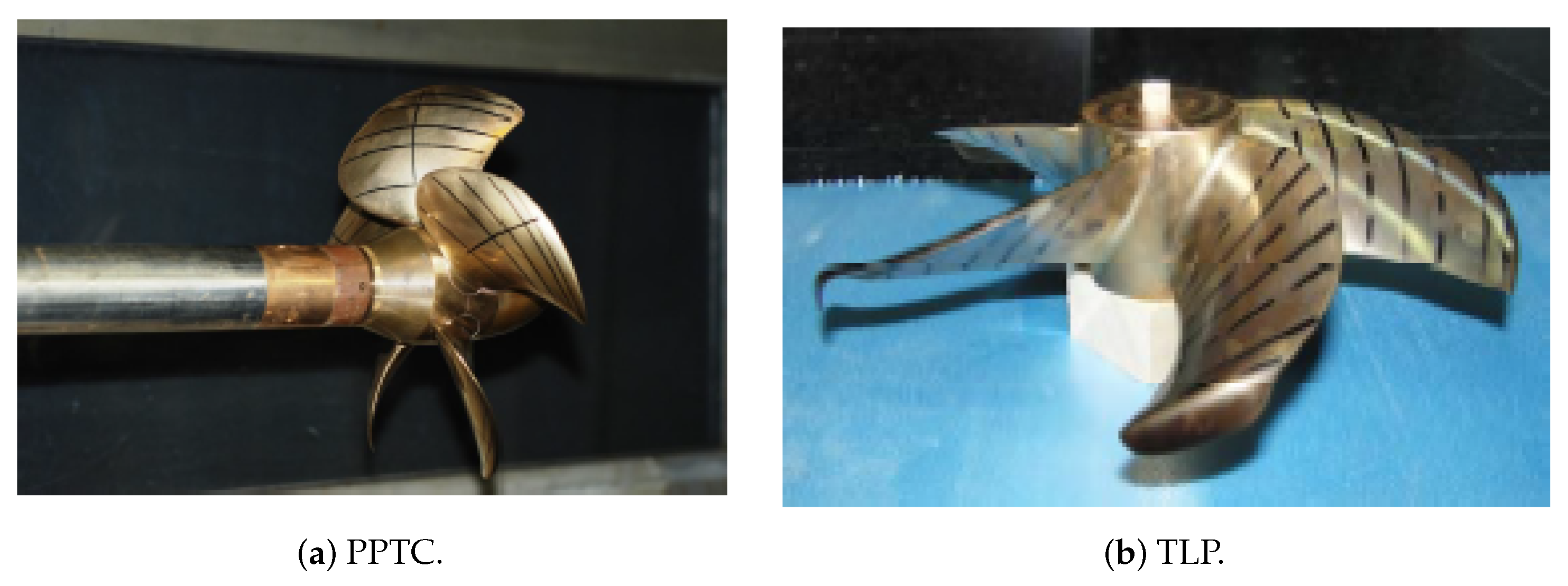
3. Test Cases
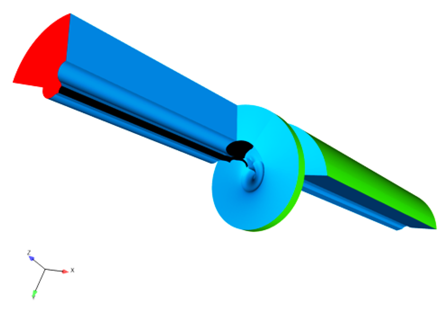
Computational Setup
4. Validation of the Numerical Method
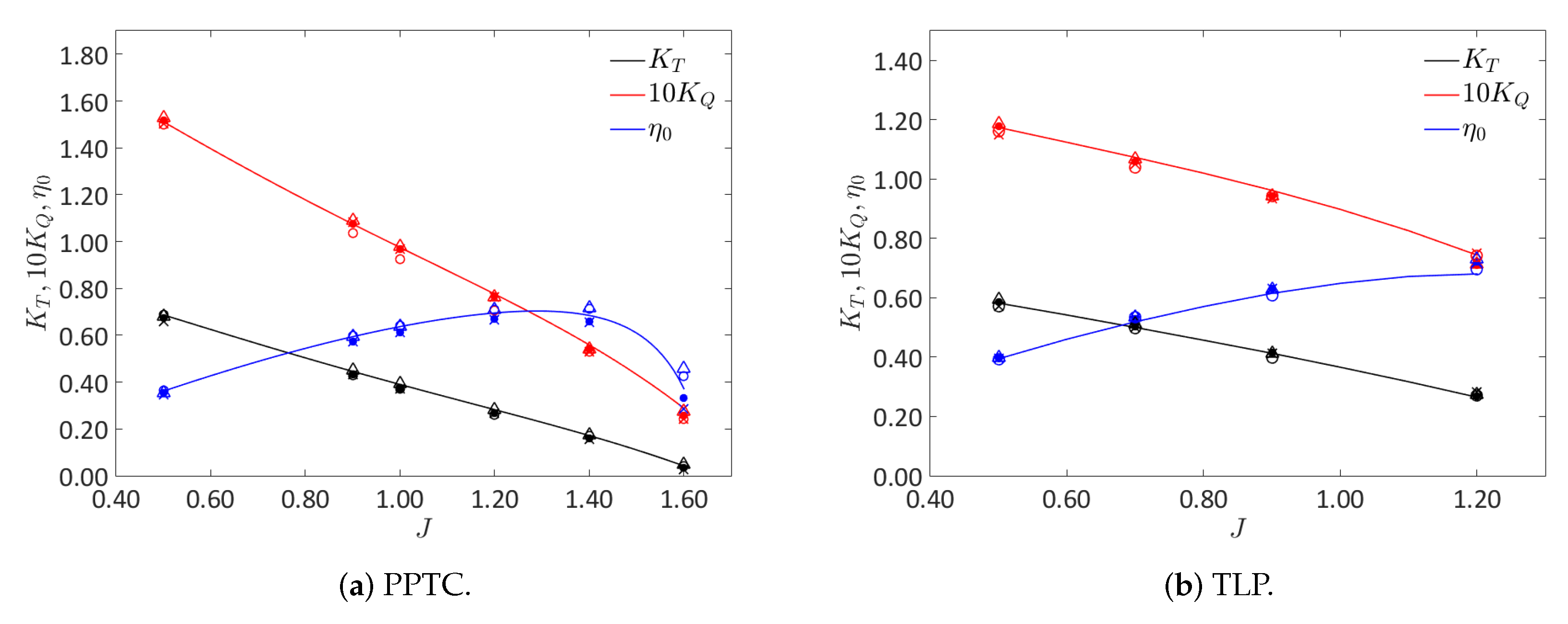
4.1. Global Forces
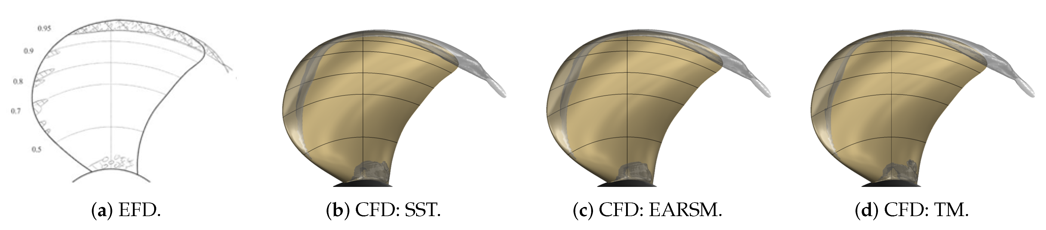
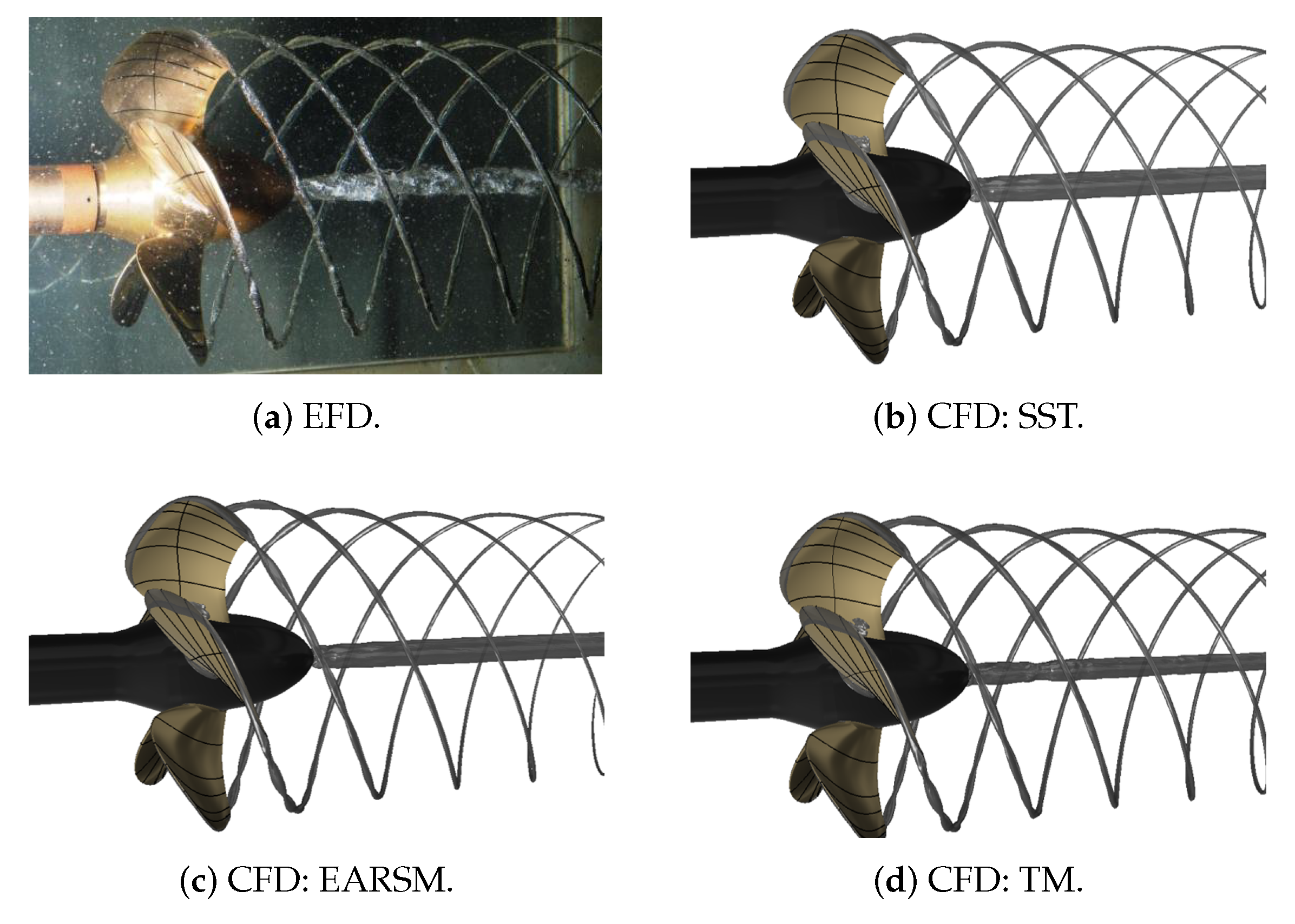
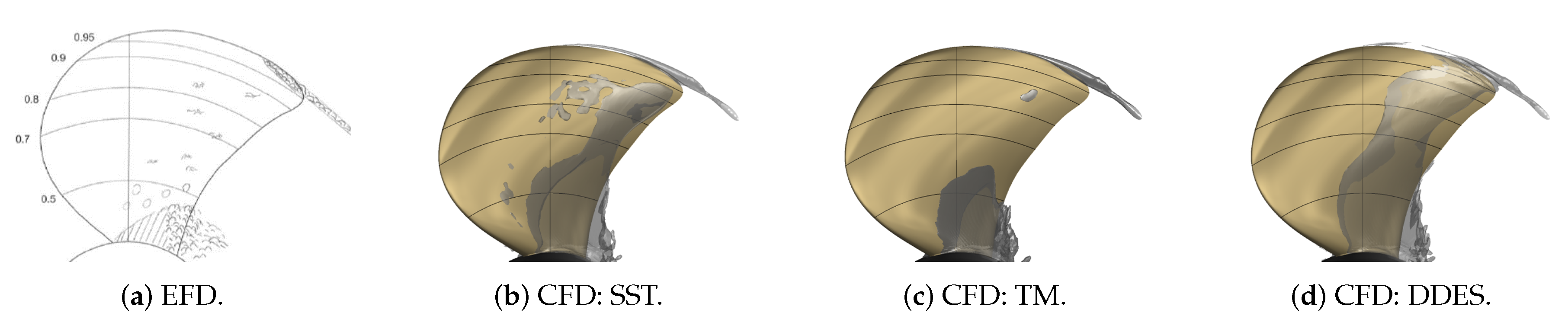
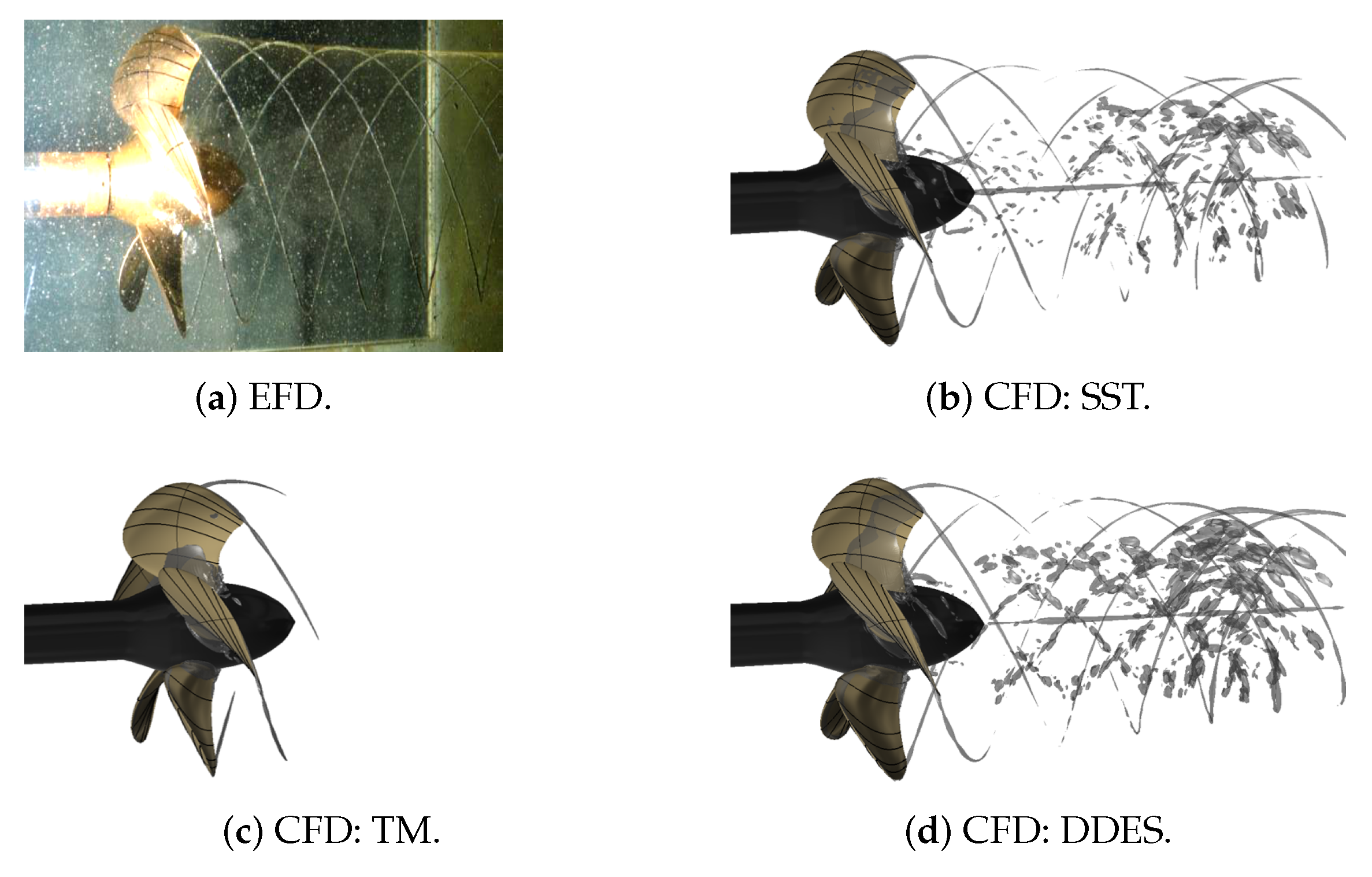
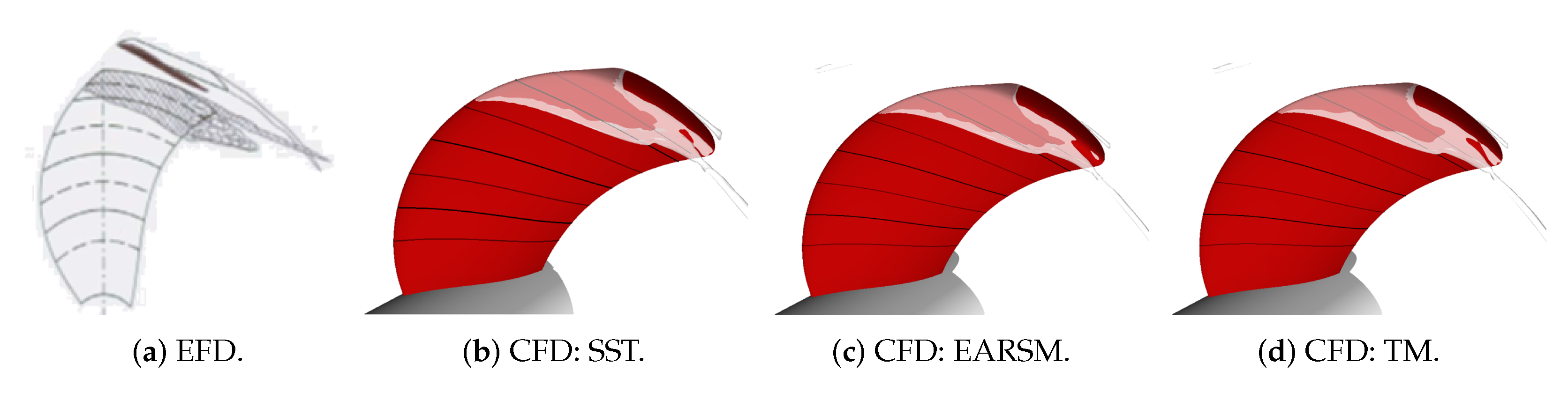
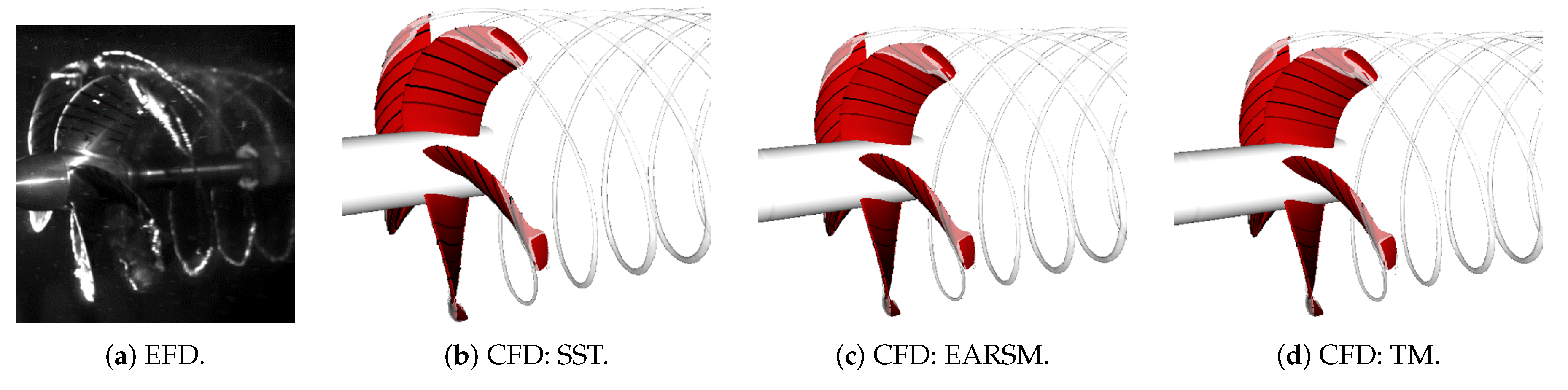
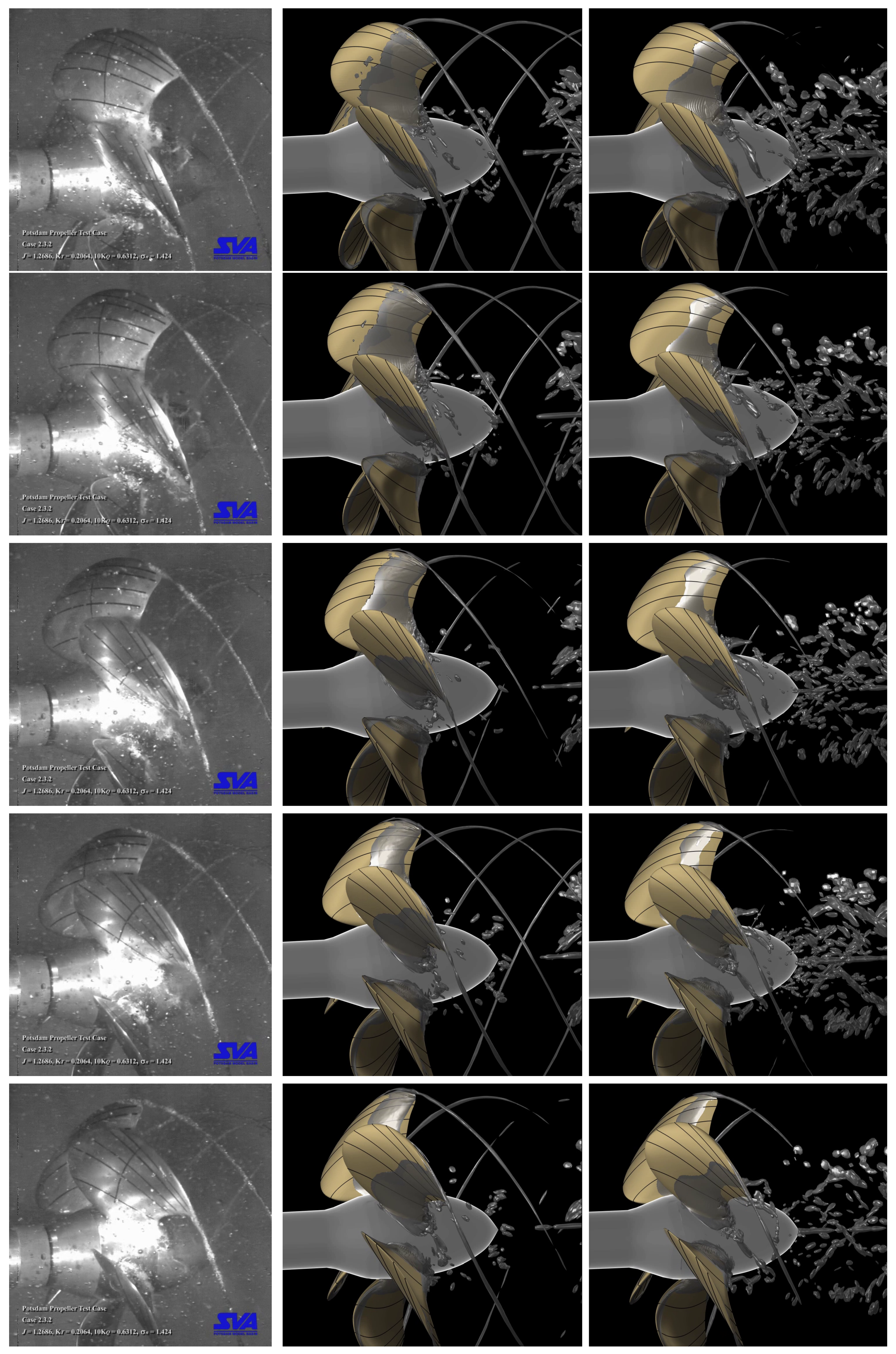
4.2. Cavitation Observation
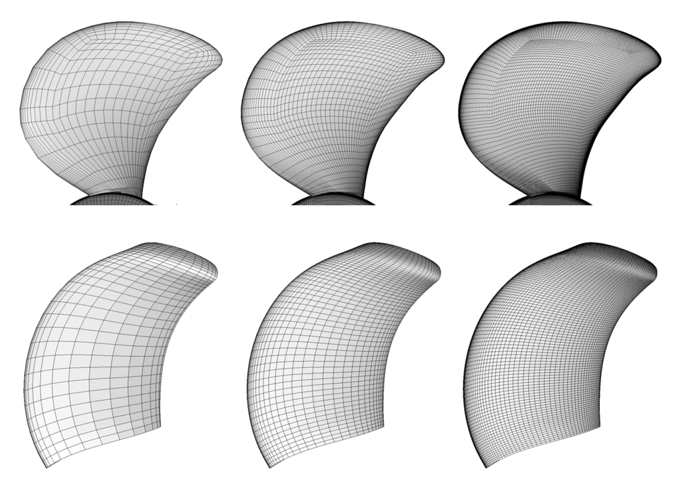
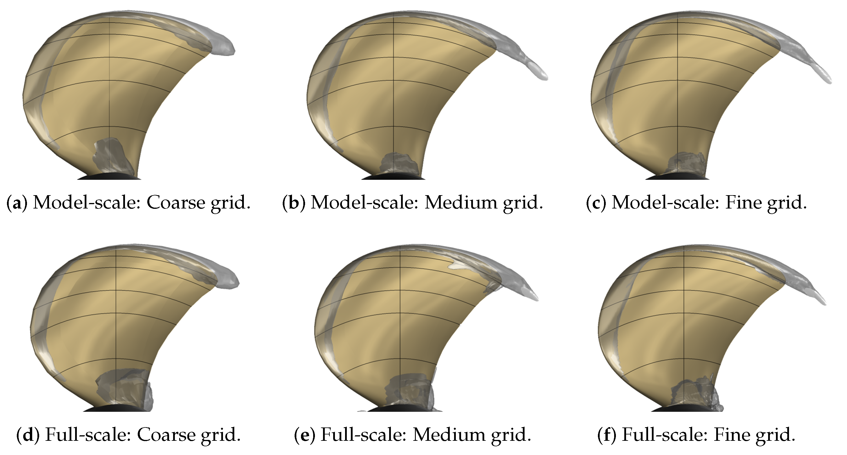
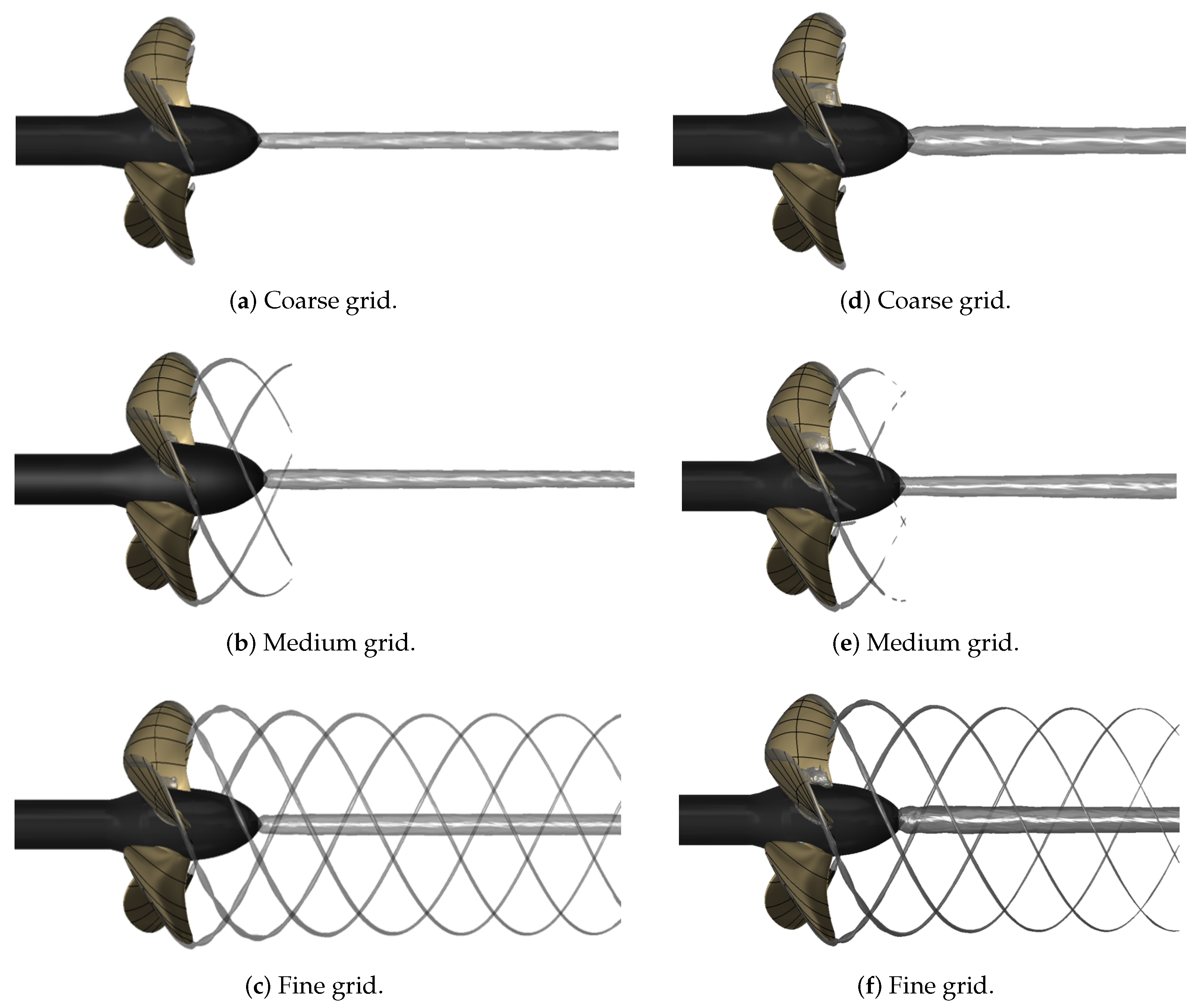
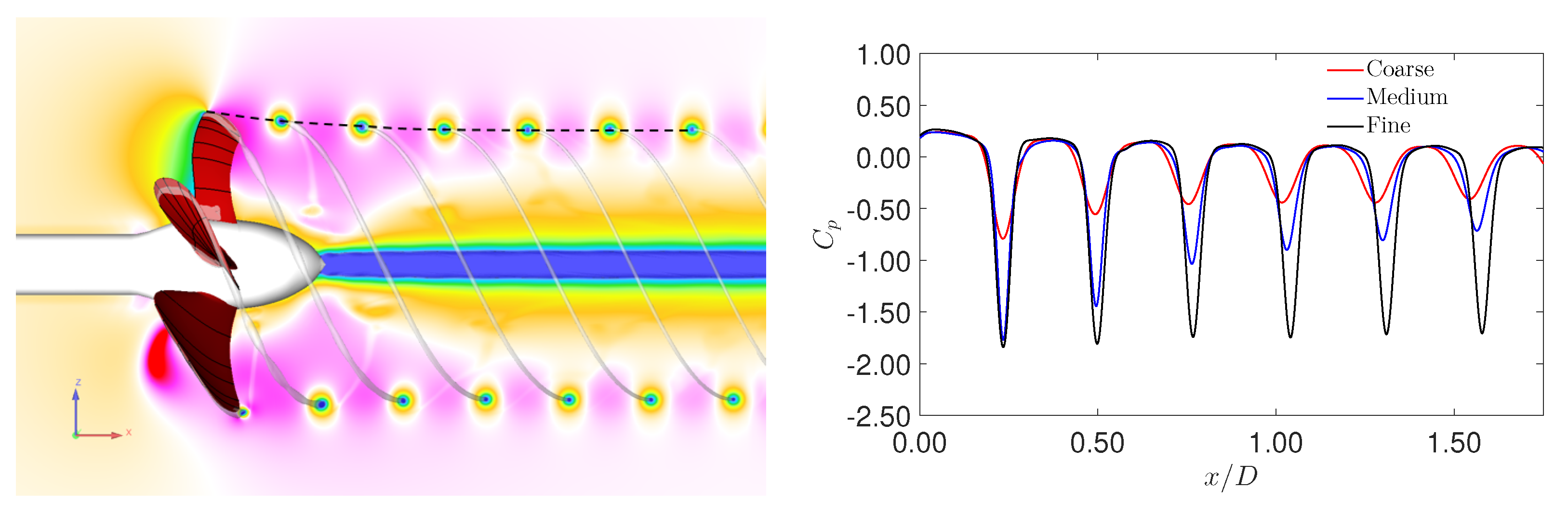
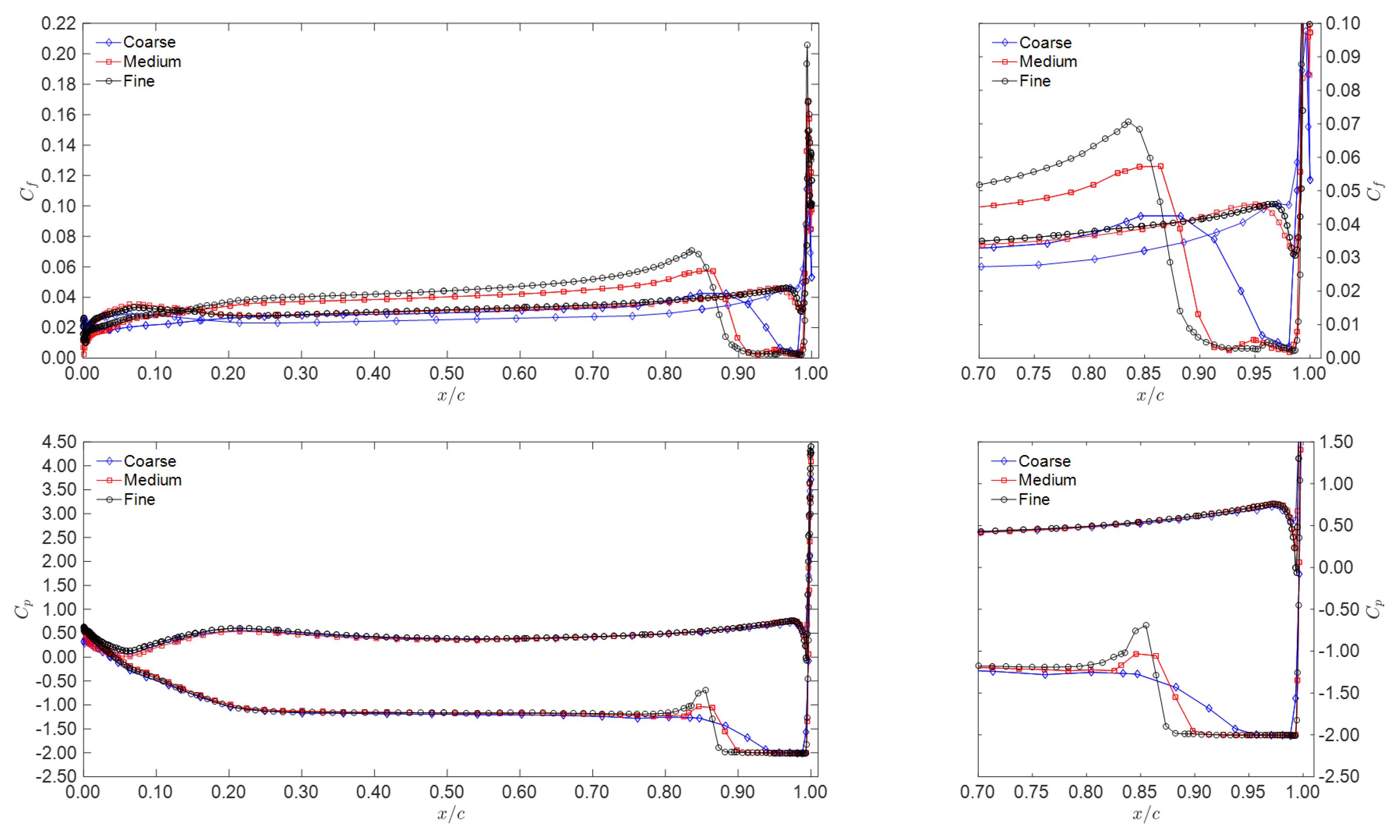
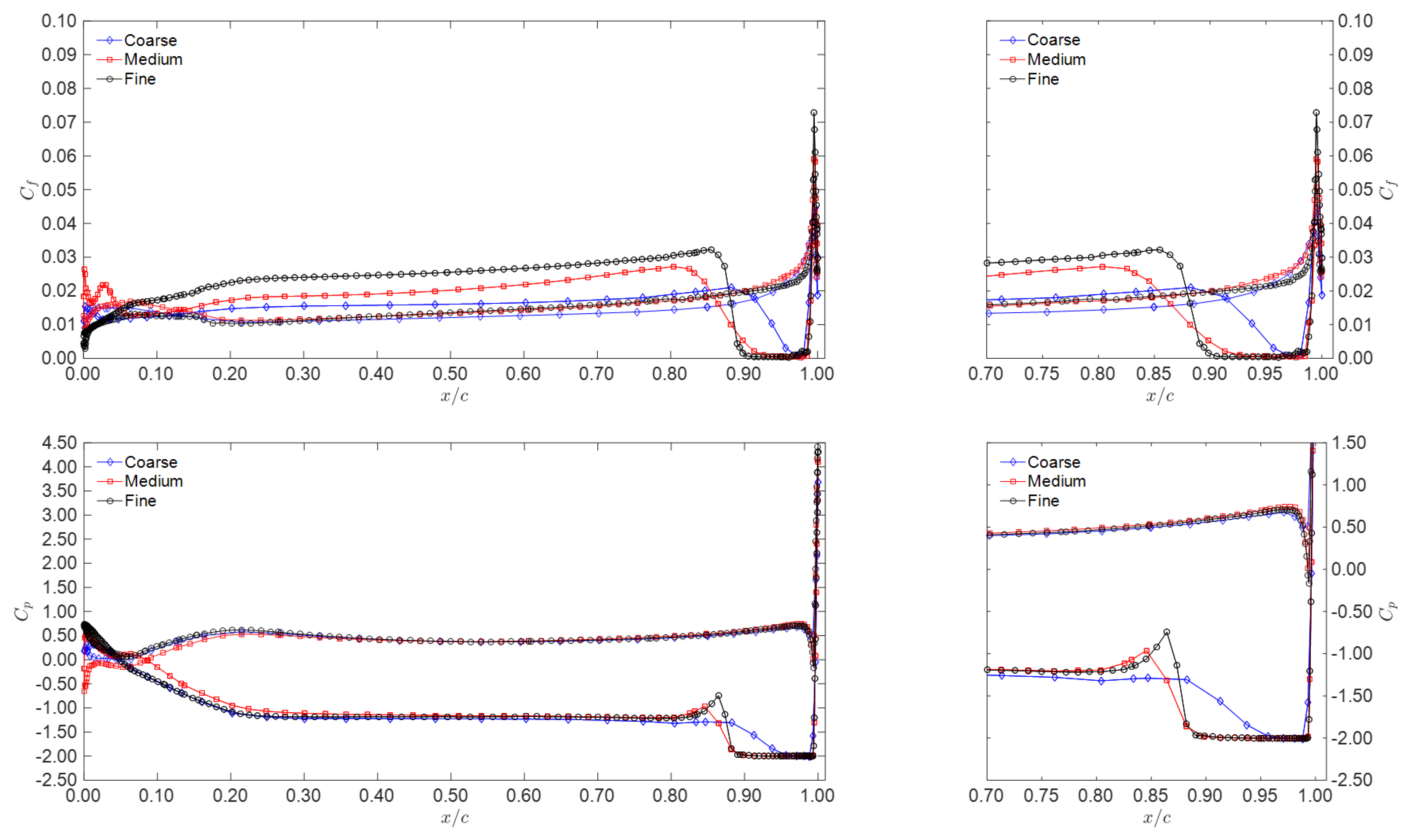
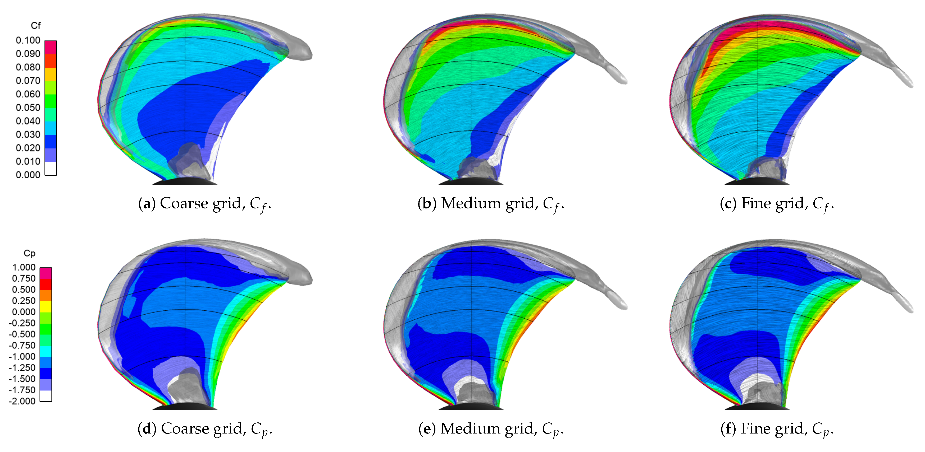
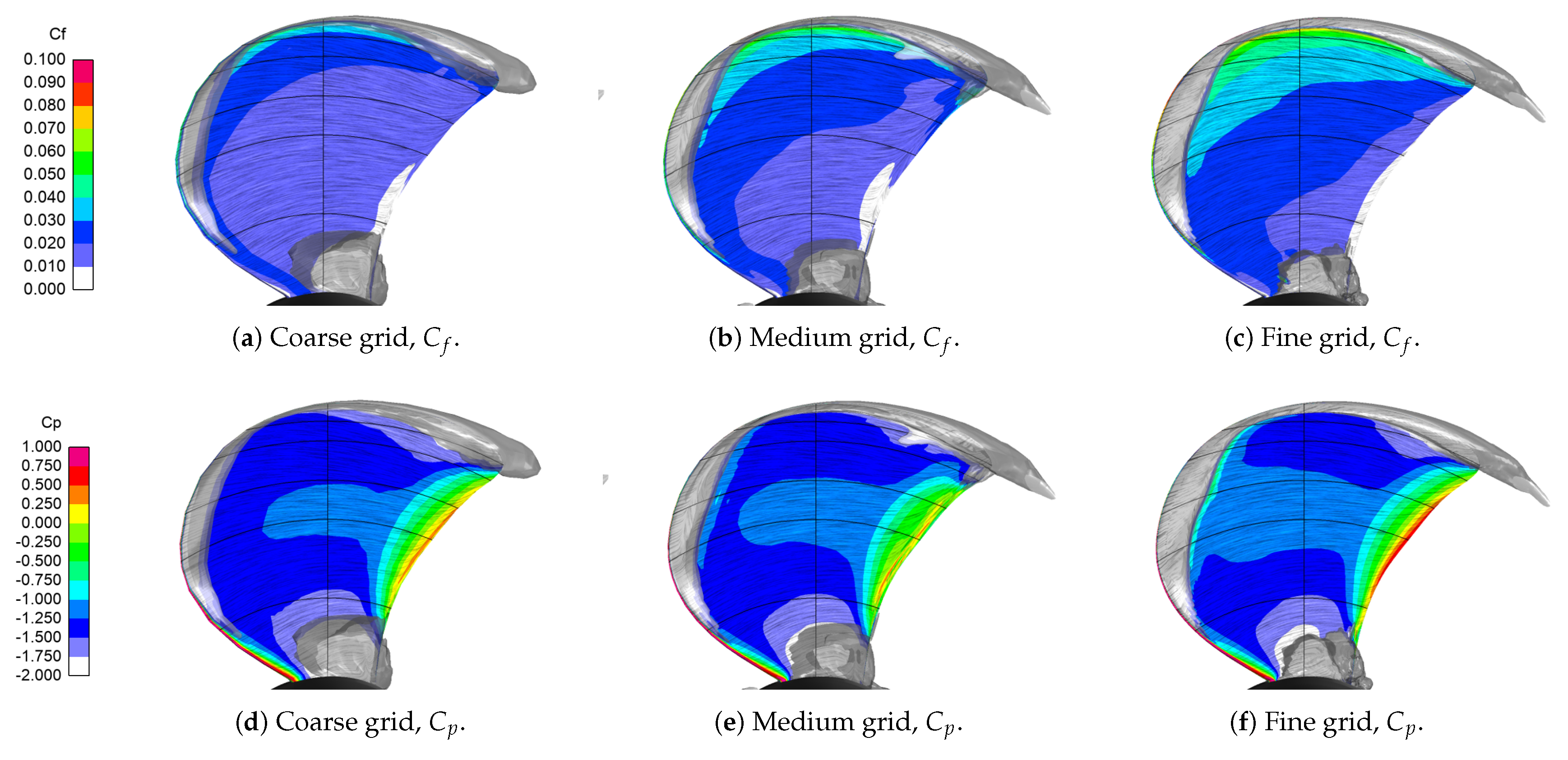
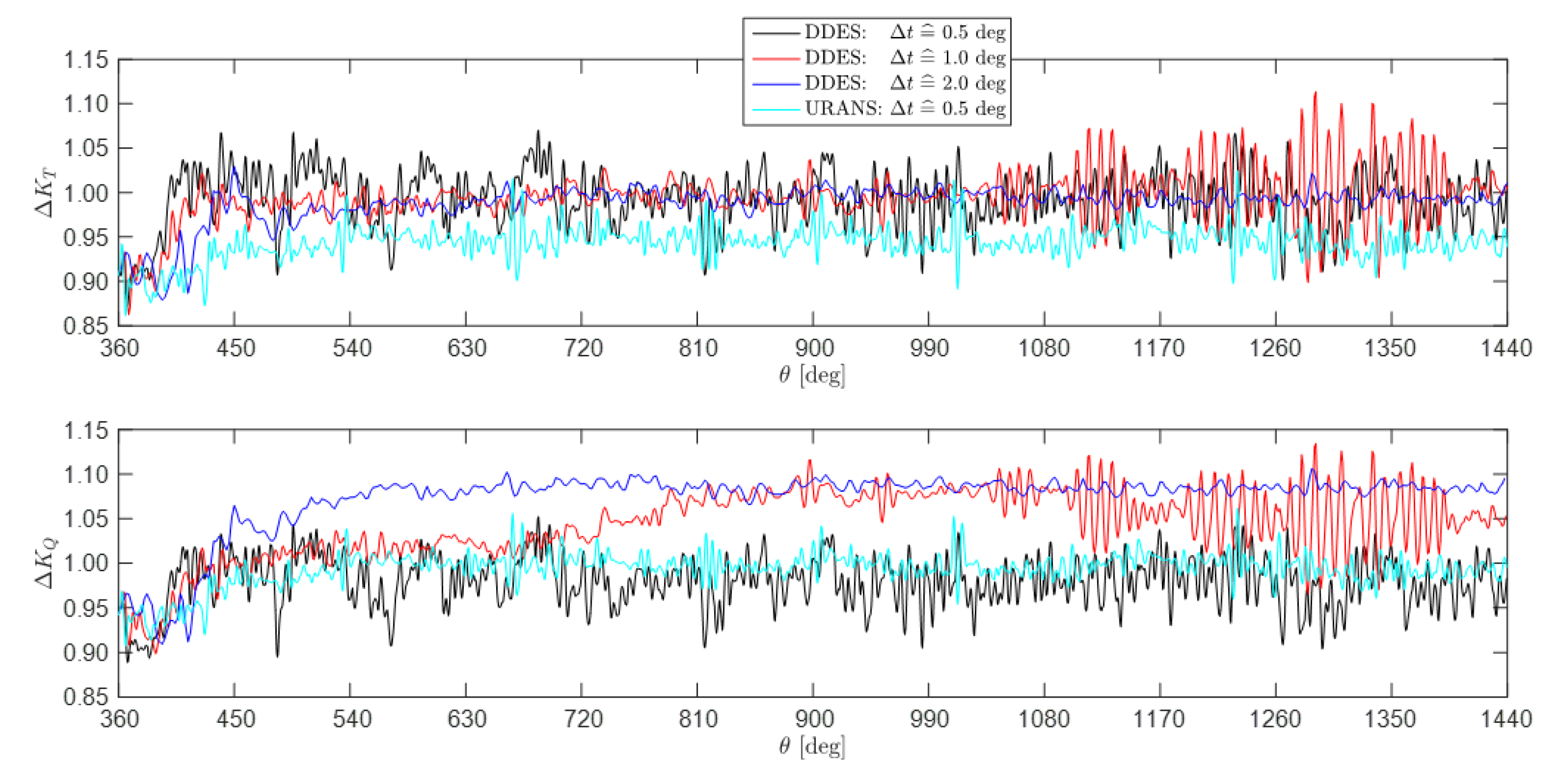
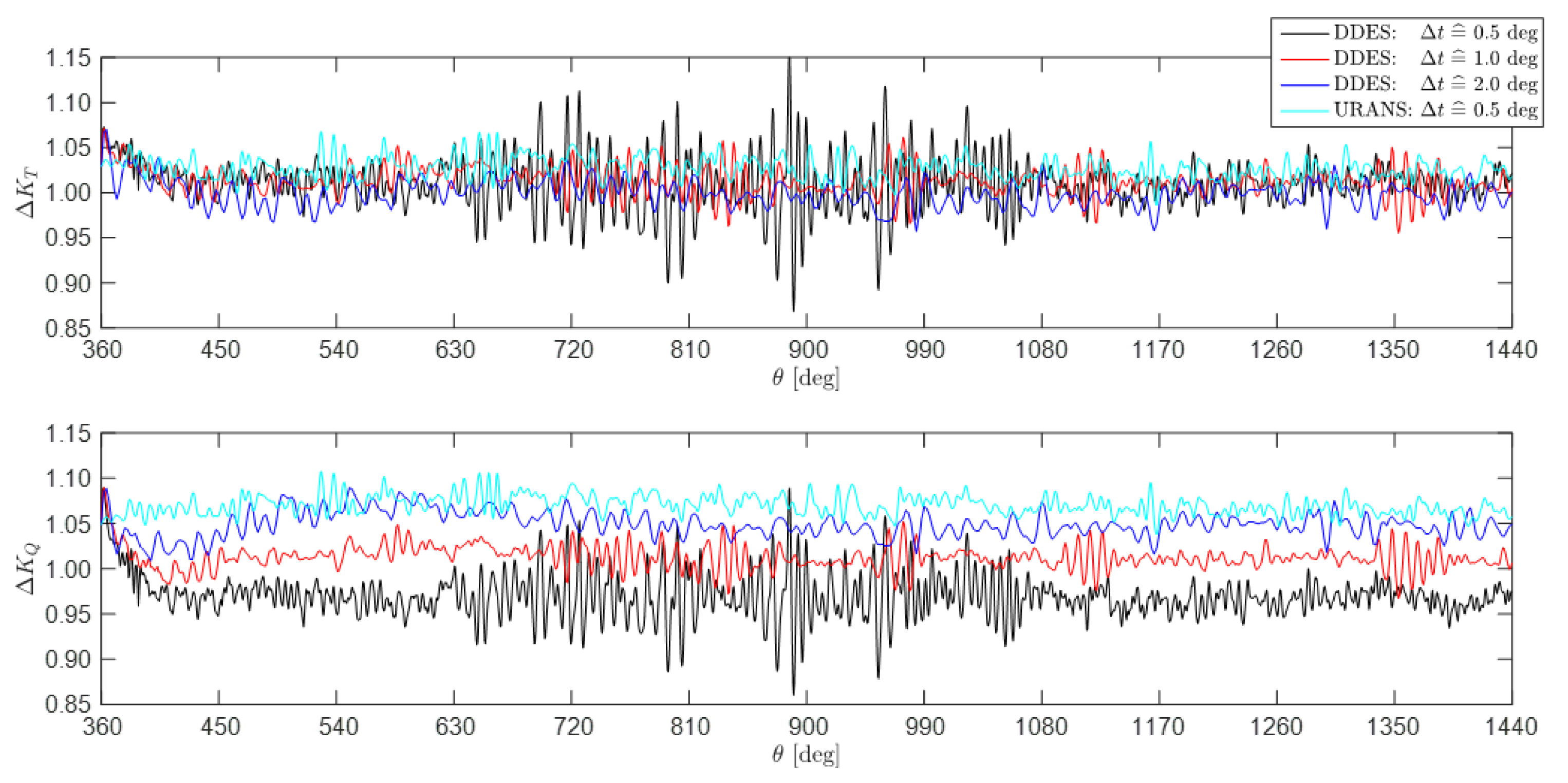
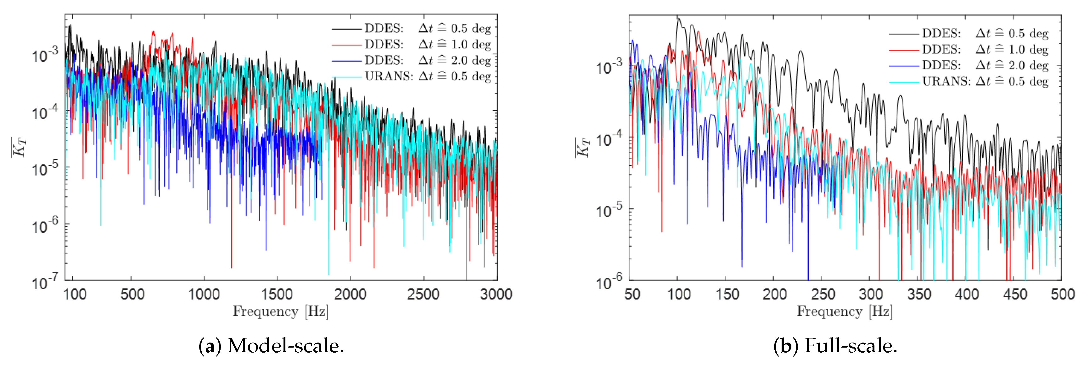
4.3. A Grid and Time Step Sensitivity Study in Model- and Full-Scale Conditions
5. Model- and Full-Scale Propeller Cavitation
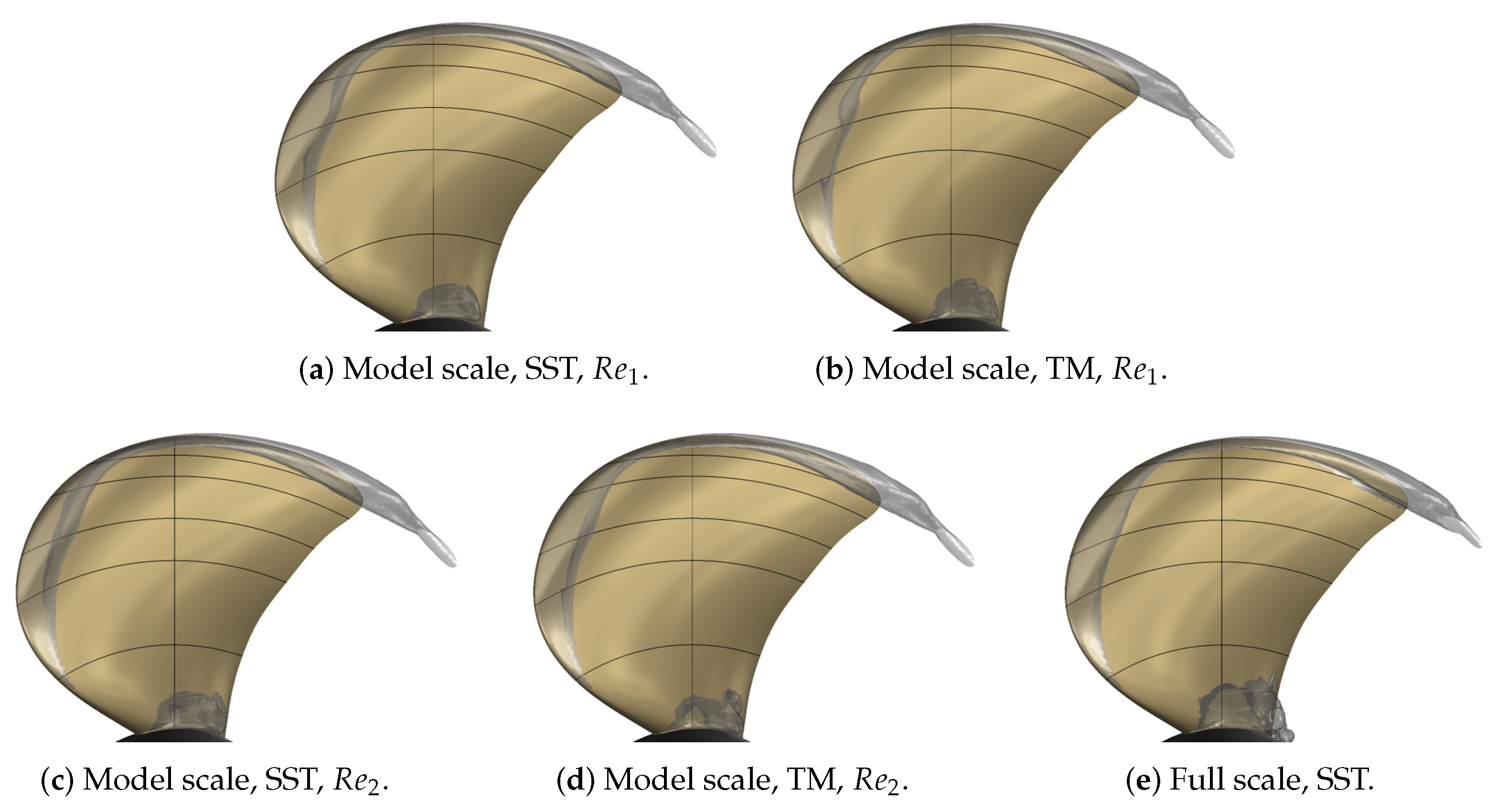
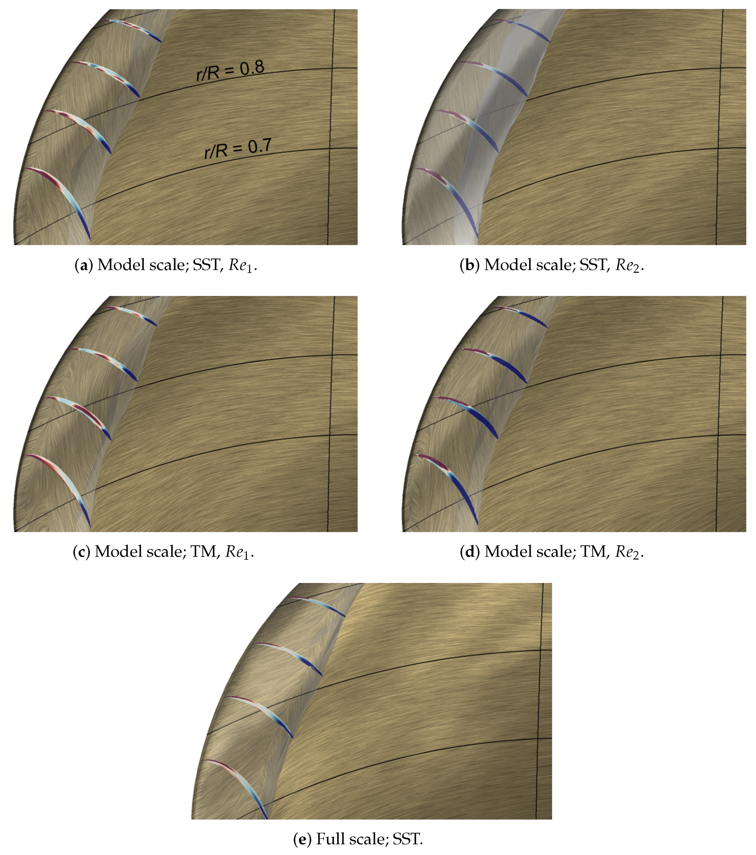
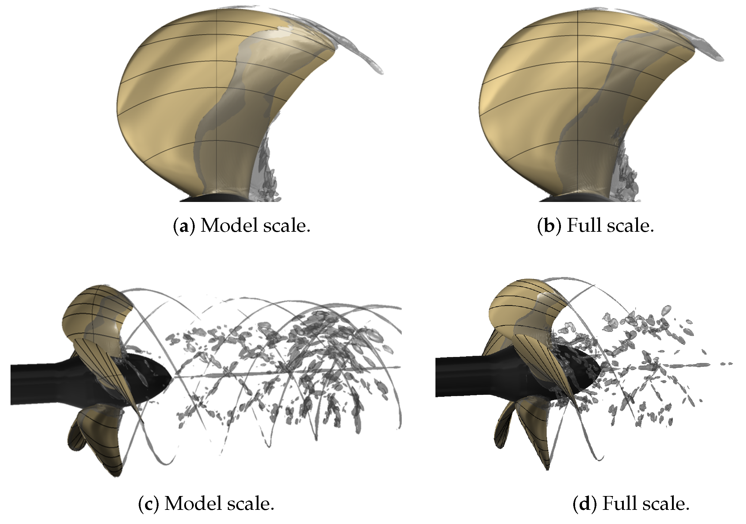
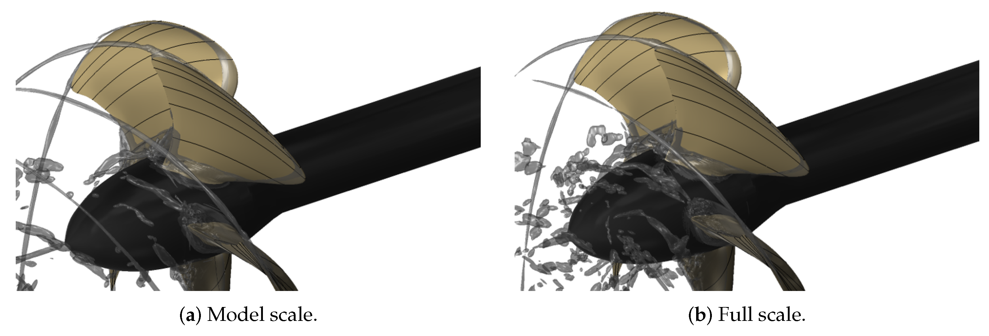
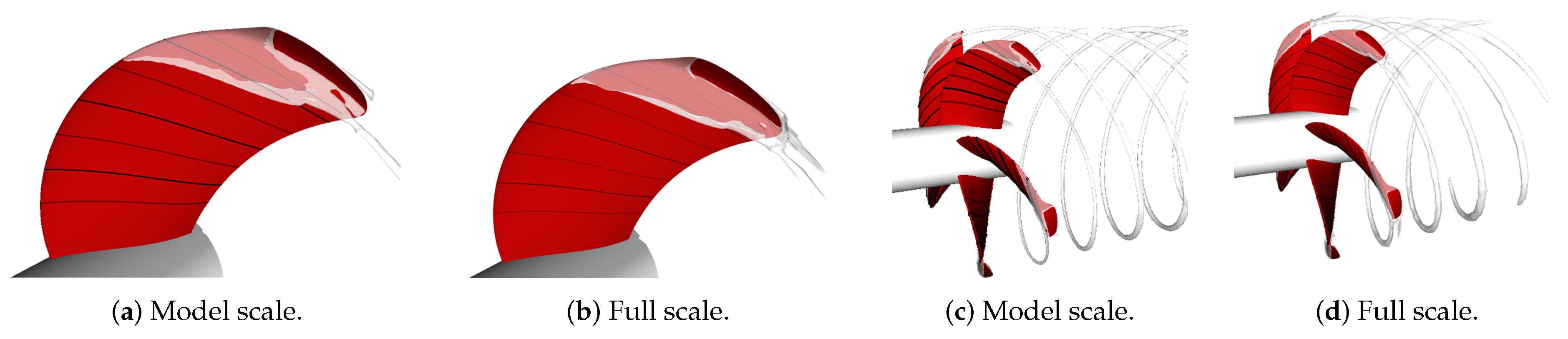
5.1. Cavitation Patterns for PPTC Propeller, Case 1 Conditions
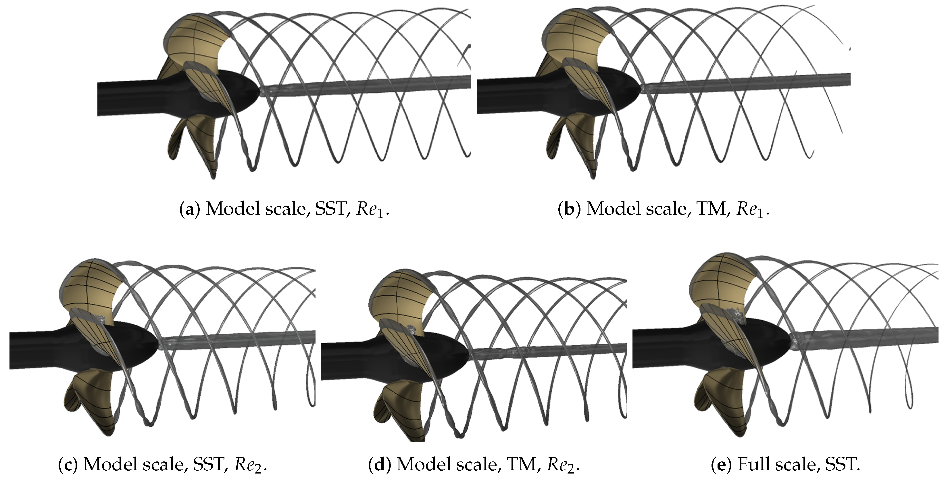
5.2. Cavitation Patterns for PPTC Propeller, Case 2 Conditions
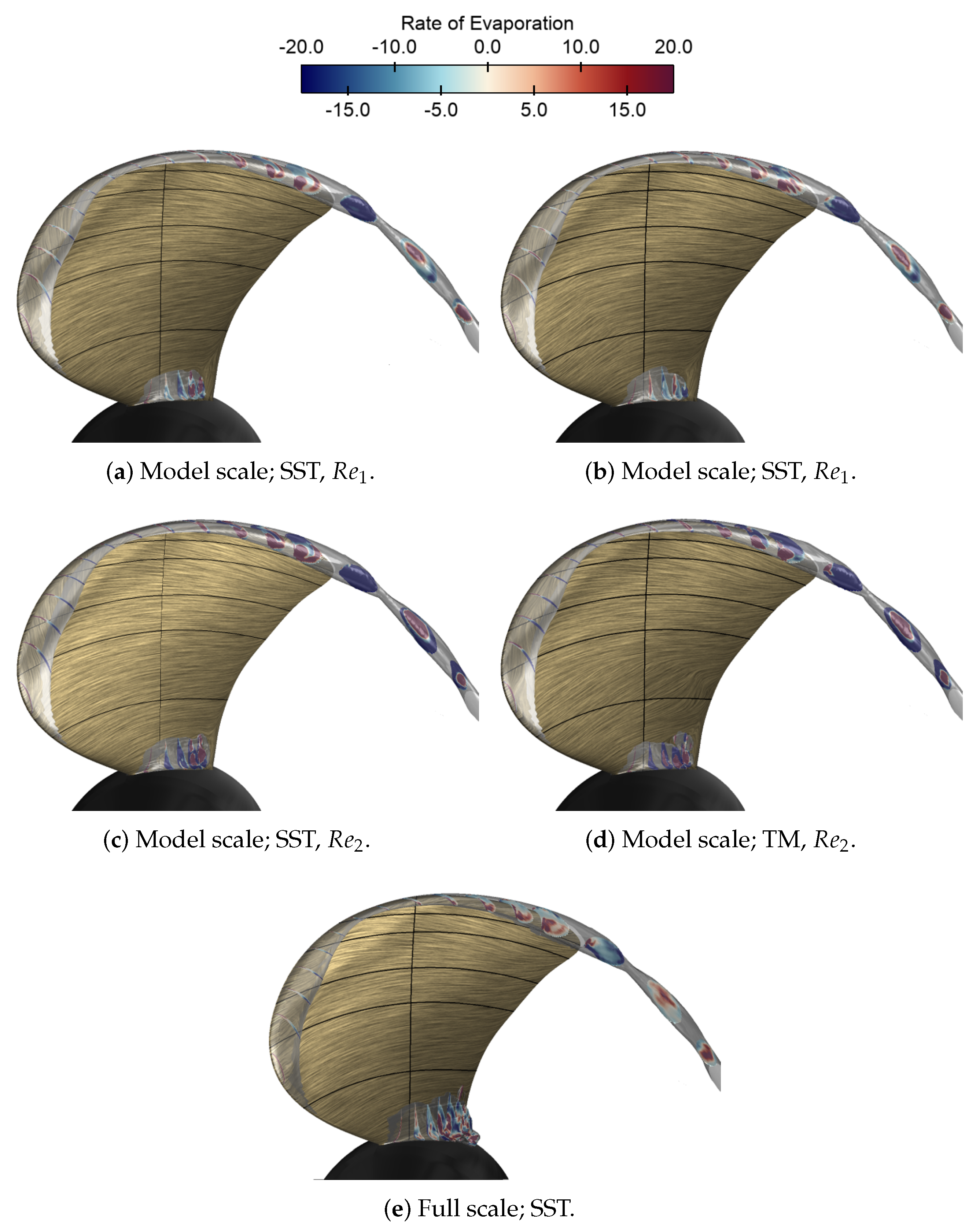
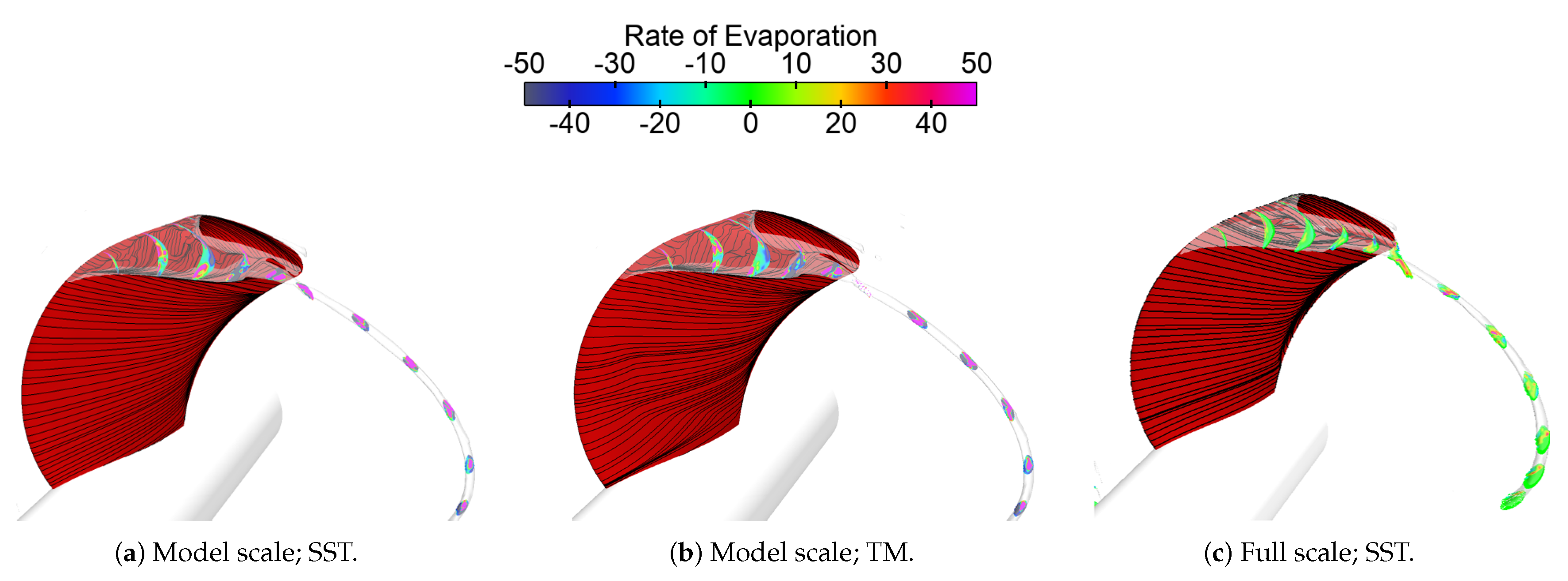
5.3. Cavitation Patterns and Evaporation Rate for TLP Propeller
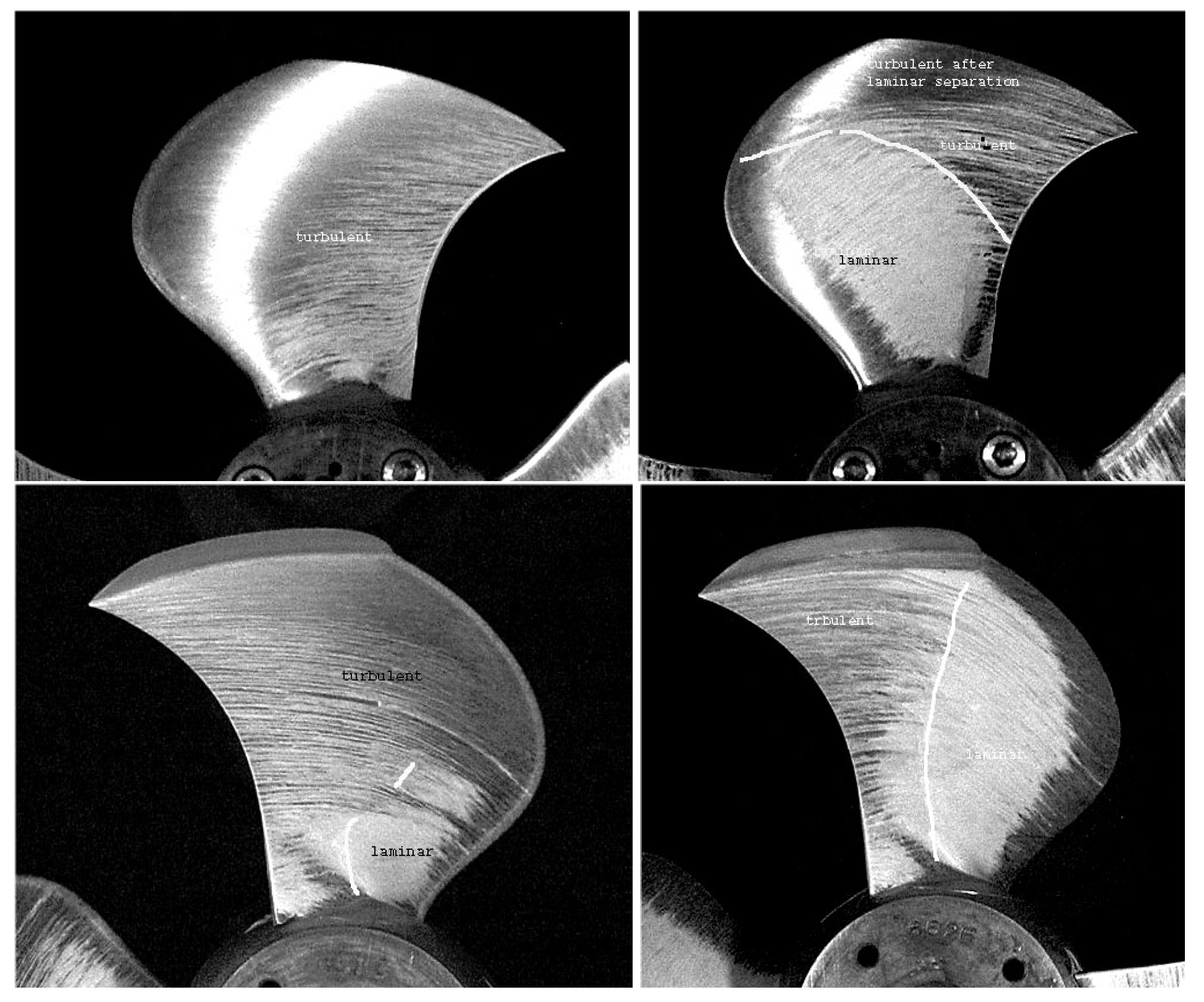
6. Near-Blade Flow: Skin-Friction and Pressure Distributions
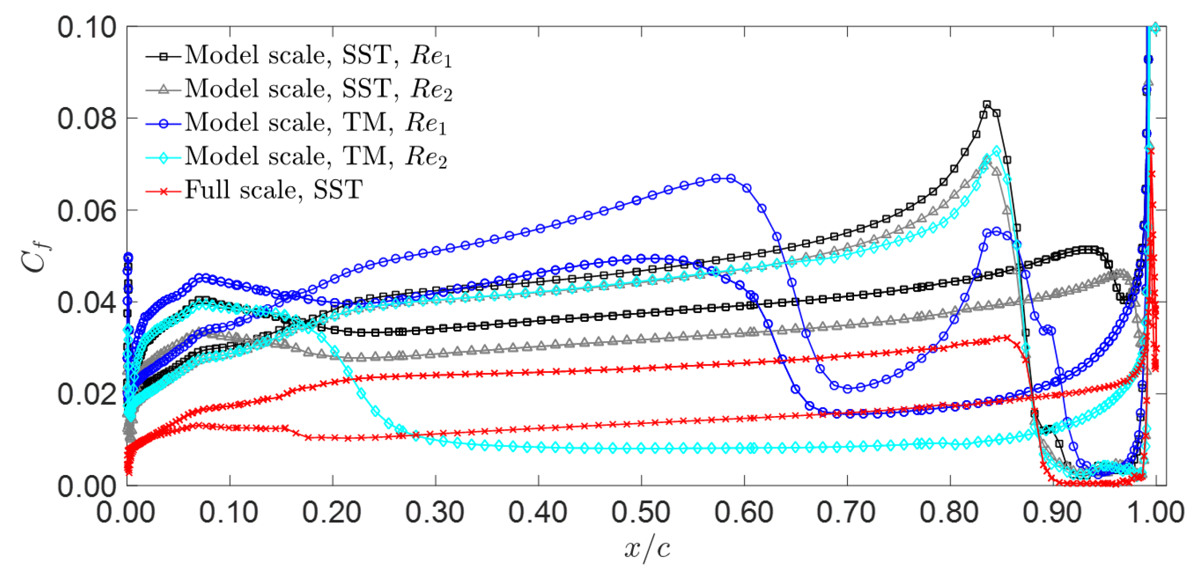
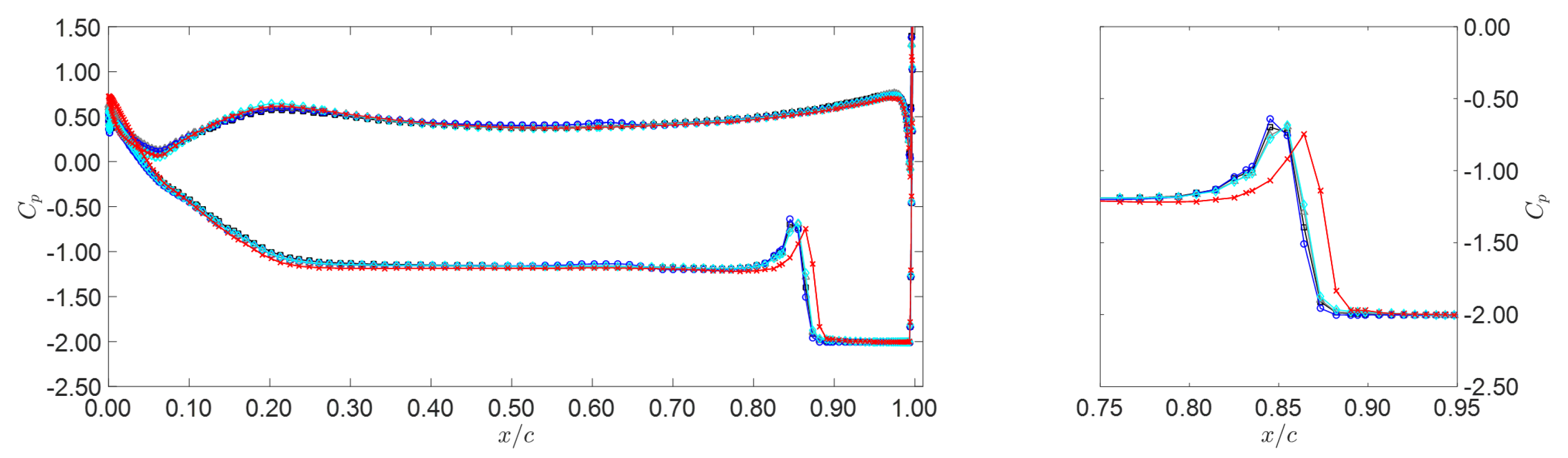
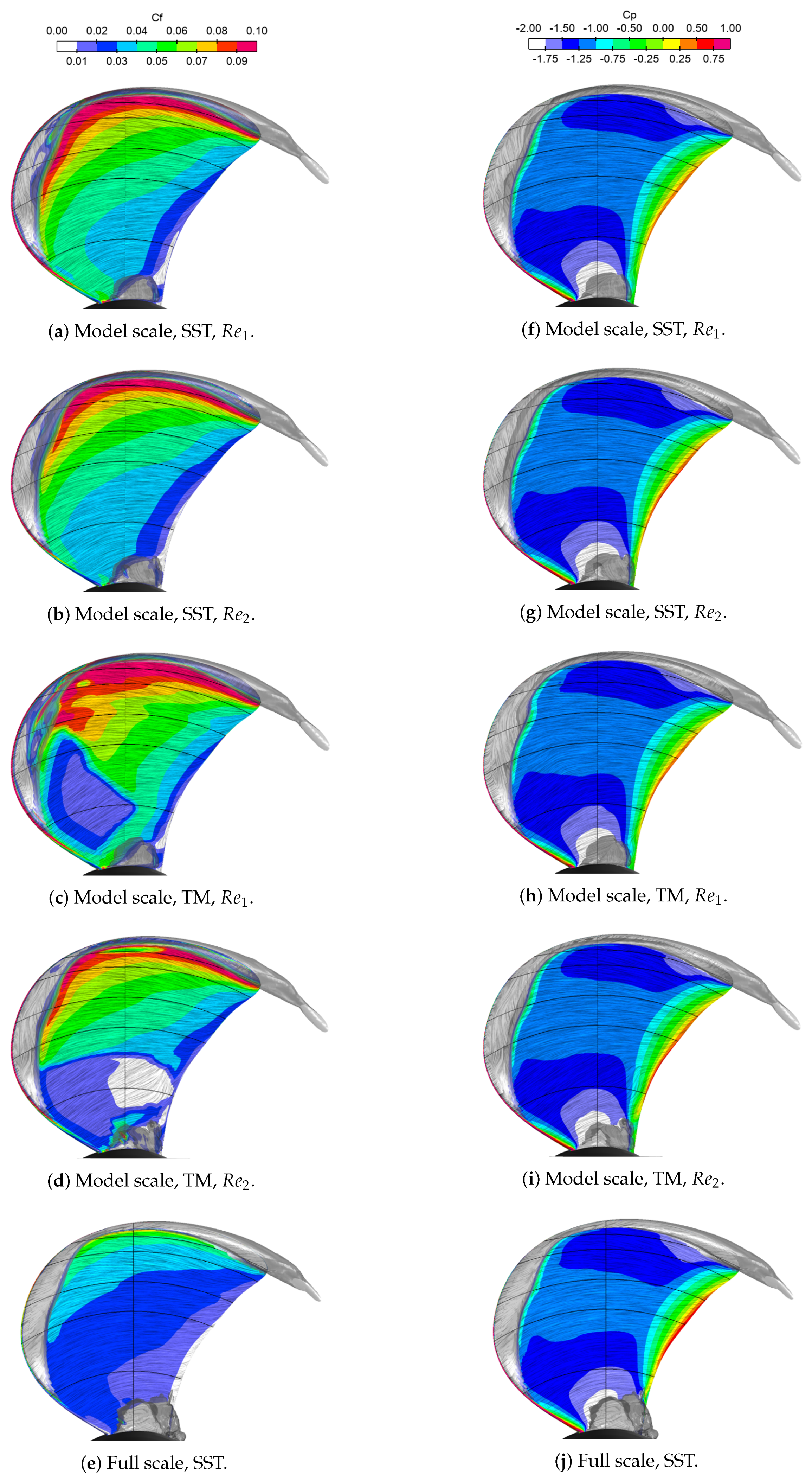
6.1. Near-Blade Flow Analysis for PPTC
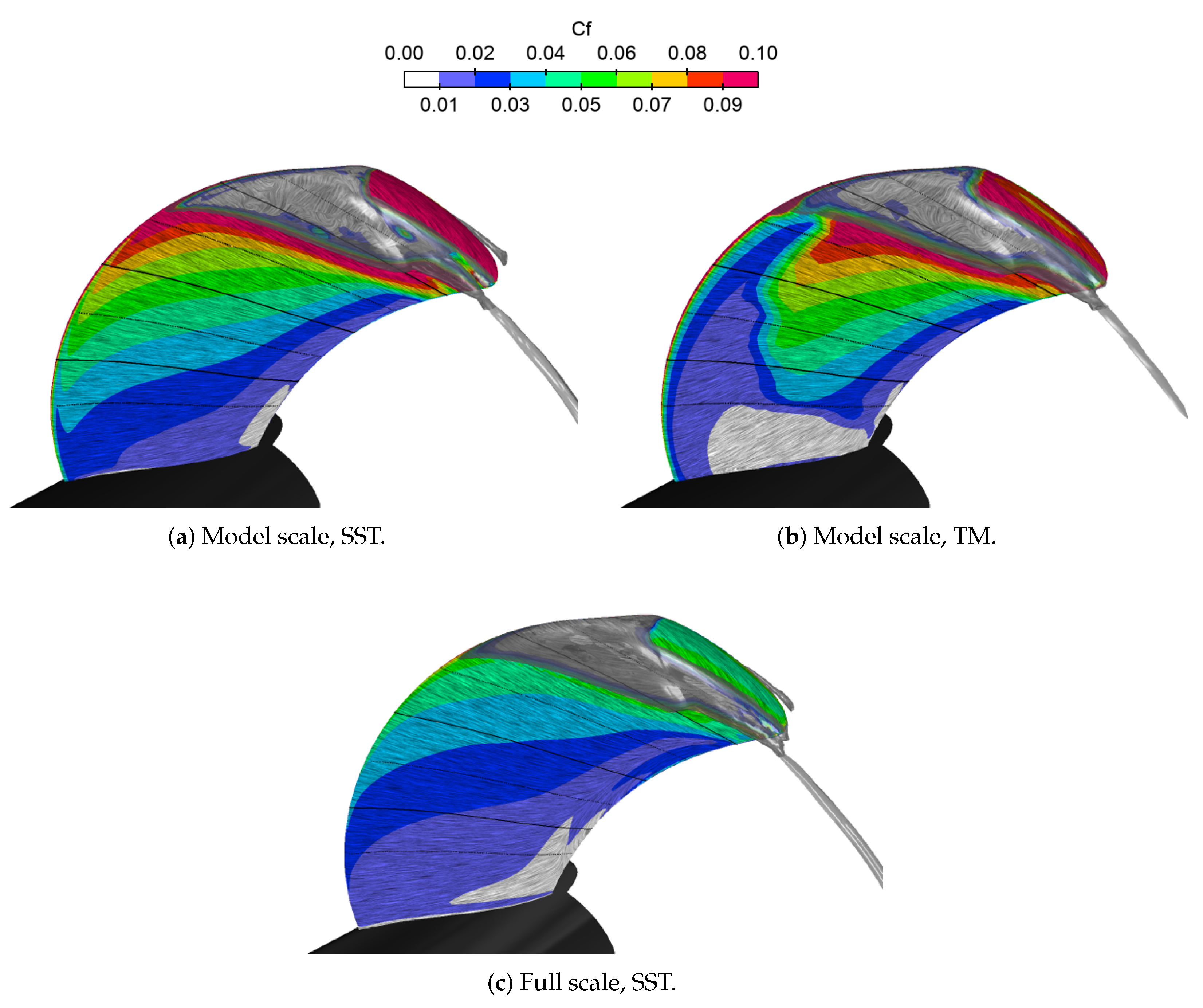
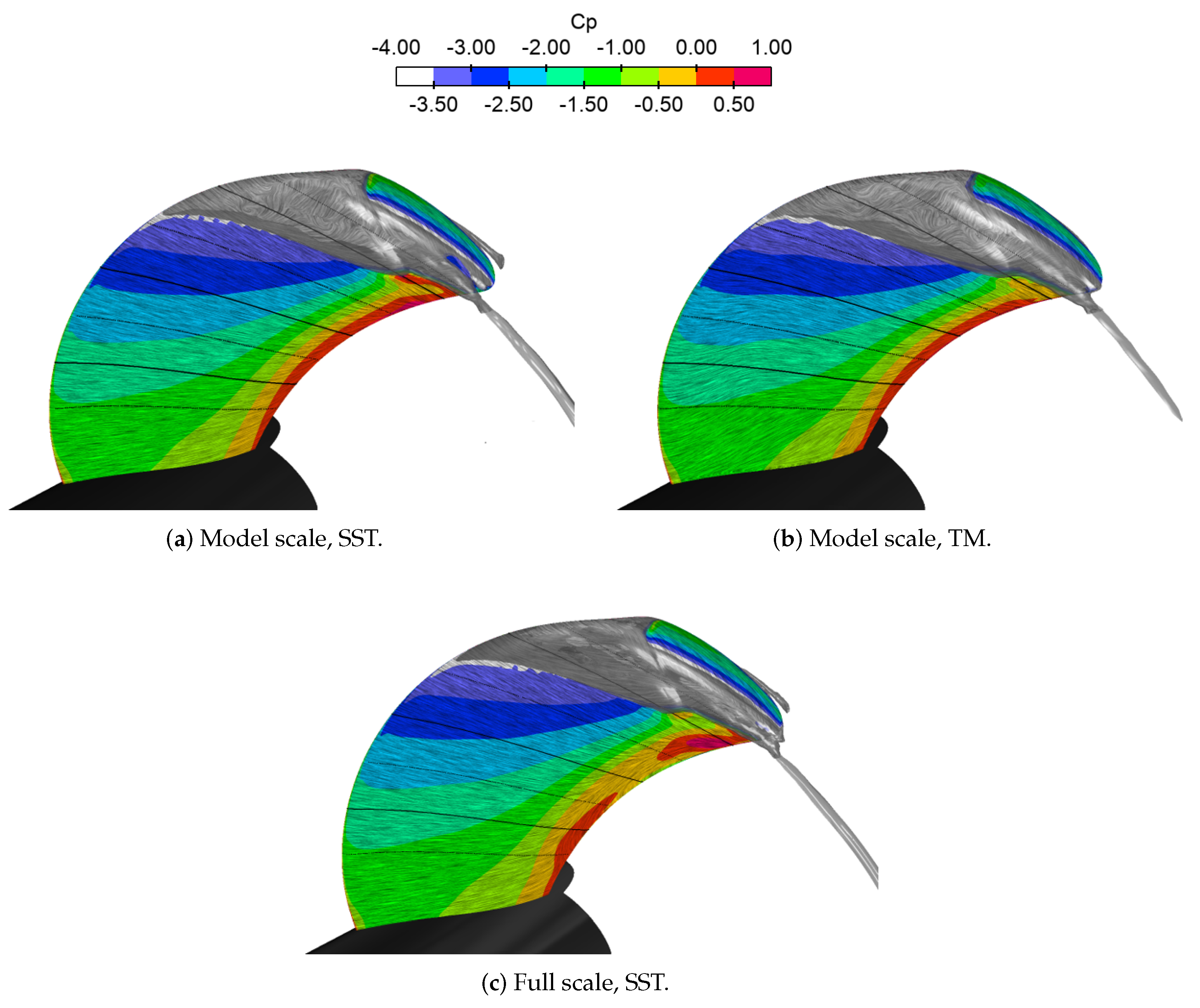
6.2. Near-Blade Flow Analysis for TLP
7. Discussion and Conclusions
Author Contributions
Funding
Acknowledgments
Conflicts of Interest
Abbreviations
| CFD | Computational fluid dynamics |
| CLT | Contracted and loaded tip |
| CPU | Centra processing unit |
| DES | Detached eddy simulation |
| DDES | Delayed detached eddy simulation |
| EARSM | Explicit algebraic Reynolds stress model |
| EFD | Experimental fluid dynamics |
| LDV | Laser Doppler velocimetry |
| LE | Leading edge |
| LES | Large eddy simulation |
| MUSCL | Monotonic upstream-centred scheme for conservation laws |
| PPTC | Potsdam propeller test case |
| RANS | Reynolds averaged Navier–Stokes |
| SST | Shear stress transport |
| TE | Trailing edge |
| TLP | Tip loaded propeller |
| TM | Transition model |
References
- Rijpkema, D.; Baltazar, J.; Falcão de Campos, J. Viscous flow simulations of propellers in different Reynolds number regimes. In Proceedings of the Fourth International Symposium on Marine Propulsors, Austin, TX, USA, 31 May–June 4 2015. [Google Scholar]
- Sánchez-Caja, A.; González-Adalid, J.; Pérez-Sobrino, M.; Sipilä, T. Scale effects on tip loaded propeller performance using a RANSE solver. Ocean Eng. 2014, 88, 607–617. [Google Scholar] [CrossRef]
- Dong, X.Q.; Li, W.; Yang, C.J.; Noblesse, F. RANSE-based Simulation and Analysis of Scale Effects on Open-Water Performance of the PPTC-II Benchmark Propeller. J. Ocean Eng. Sci. 2018, 3, 186–204. [Google Scholar] [CrossRef]
- Müller, S.B.; Abdel-Maksoud, M.; Hilbert, G. Scale effects on propellers for large container vessels. In Proceedings of the First Internatioal Symposium on Marine Propulsors, Trondheim, Norway, 22–24 June 2009. [Google Scholar]
- Baltazar, J.; Rijpkema, D.; Falcão de Campos, J. On the use of the γ − Reθ transition model for the prediction of the propeller performance at model-scale. Ocean Eng. 2018, 170, 6–19. [Google Scholar] [CrossRef]
- Baltazar, J.; Rijpkema, D.; Falcão de Campos, J. Prediction of the Propeller Performance at Different Reynolds Number Regimes with RANS. In Proceedings of the 6th International Symposium on Marine Propulsors, SMP’19, Rome, Italy, 26–30 May 2019. [Google Scholar]
- Amromin, E. Estimations of scale effects on blade cavitation. J. Phys. Conf. Ser. IOP Publ. 2015, 656. [Google Scholar] [CrossRef]
- Viitanen, V.; Siikonen, T.; Sánchez-Caja, A. Numerical Viscous Flow Simulations of Cavitating Propeller Flows at Different Reynolds Numbers. In Proceedings of the 6th International Symposium on Marine Propulsors, SMP’19, Rome, Italy, 26–30 May 2019. [Google Scholar]
- Miettinen, A.; Siikonen, T. Application of pressure- and density-based methods for different flow speeds. Int. J. Numer. Methods Fluids 2015, 79, 243–267. [Google Scholar] [CrossRef]
- Viitanen, V.M.; Siikonen, T. Numerical simulation of cavitating marine propeller flows. In Proceedings of the 9th National Conference on Computational Mechanics (MekIT’17), Trondheim, Norway, 11–12 May 2017; International Center for Numerical Methods in Engineering (CIMNE): Trondheim, Norway, 2017; pp. 385–409, ISBN 978-84-947311-1-2. [Google Scholar]
- Miettinen, A. Simple Polynomial Fittings for Steam, CFD/THERMO-55-2007; Report 55; Laboratory of Applied Thermodynamics, Aalto University: Espoo, Finland, 2007. [Google Scholar]
- Spalart, P.R.; Deck, S.; Shur, M.; Squires, K.; Strelets, M.K.; Travin, A. A new version of detached-eddy simulation, resistant to ambiguous grid densities. Theor. Comput. Fluid Dyn. 2006, 20, 181–195. [Google Scholar] [CrossRef]
- Menter, F.R. Two-equation eddy-viscosity turbulence models for engineering applications. AIAA J. 1994, 32, 1598–1605. [Google Scholar] [CrossRef] [Green Version]
- Langtry, R.B. A Correlation-Based Transition Model Using Local Variables for Unstructured Parallelized CFD Codes. Ph.D. thesis, University of Stuttgart, Stuttgart, Germany, 2006. [Google Scholar]
- Menter, F.; Langtry, R.; Likki, S.; Suzen, Y.; Huang, P.; Völker, S. A correlation-based transition model using local variables Part I: Model formulation. J. Turbomach. 2006, 128, 413–422. [Google Scholar] [CrossRef]
- Langtry, R.; Menter, F.; Likki, S.; Suzen, Y.; Huang, P.; Völker, S. A correlation-based transition model using local variables Part II: Test cases and industrial applications. J. Turbomach. 2006, 128, 423–434. [Google Scholar] [CrossRef]
- Hellsten, A. Curvature corrections for algebraic Reynolds stress modeling: A discussion. AIAA J. 2002, 40, 1909–1911. [Google Scholar] [CrossRef]
- Hellsten, A.; Wallin, S.; Laine, S. Scrutinizing curvature corrections for algebraic Reynolds stress models. In Proceedings of the 32nd AIAA Fluid Dynamics Conference, AIAA, St. Louis, MO, USA, 24–26 June 2002. AIAA Paper 2002–2963. [Google Scholar]
- Menter, F. Influence of freestream values on k − ω turbulence model predictions. AIAA J. 1992, 30, 1657–1659. [Google Scholar] [CrossRef]
- Shur, M.; Spalart, P.; Strelets, M.; Travin, A. Detached-Eddy Simulation of an Airfoil at High Angle of Attack. In Proceedings of the 4th International Symposium on Engineering Turbulence Modelling and Experiments, Ajaccio, Corsica, France, 24–26 May 1999; pp. 669–678. [Google Scholar]
- Strelets, M. Detached eddy simulation of massively separated flows. In Proceedings of the 39th AIAA Aerospace Sciences Meeting and Exhibit, Reno, NV, USA, 8–11 January 2001. AIAA Paper 2001-0879. [Google Scholar]
- Frikha, S.; Coutier-Delgosha, O.; Astolfi, J.A. Influence of the cavitation model on the simulation of cloud cavitation on 2D foil section. Int. J. Rotat. Mach. 2009, 2008. [Google Scholar] [CrossRef] [Green Version]
- Choi, Y.H.; Merkle, C.L. The application of preconditioning in viscous flows. J. Comput. Phys. 1993, 105, 207–230. [Google Scholar] [CrossRef]
- Sipilä, T. RANS Analyses of Cavitating Propeller Flows. Licentiate Thesis, School of Engineering, Aalto University, Espoo, Finland, 2012. [Google Scholar]
- Viitanen, V.M.; Hynninen, A.; Sipilä, T.; Siikonen, T. DDES of Wetted and Cavitating Marine Propeller for CHA Underwater Noise Assessment. J. Marine Sci. Eng. 2018, 6, 56. [Google Scholar] [CrossRef] [Green Version]
- Heinke, H.J. Potsdam Propeller Test Case (PPTC). Cavitation Tests with the Model Propeller VP1304; SVA Potsdam Model Basin Report No.3753; Schiffbau-Versuchsanstalt Potsdam GmbH: Potsdam, Germany, 2011. [Google Scholar]
- Viitanen, V.; Hynninen, A.; Lübke, L.; Klose, R.; Tanttari, J.; Sipilä, T.; Siikonen, T. CFD and CHA simulation of underwater noise induced by a marine propeller in two-phase flows. In Proceedings of the Fifth International Symposium on Marine Propulsors (smp’17), Espoo, Finland, 12–15 June 2017. [Google Scholar]


| Diameter [m] | 0.250 |
| Pitch ratio at | 1.635 |
| Chord at | 0.417 |
| EAR | 0.779 |
| Skew | 18.837 |
| Hub ratio | 0.300 |
| Number of blades | 5 |
| Rotation | Right-handed |
| Diameter [m] | 0.250 |
| Pitch ratio at | 1.465 |
| EAR | 0.594 |
| Number of blades | 5 |
| Rotation | Right-handed |
| Quantity | PPTC, Case 1 | PPTC, Case 2 | TLP |
|---|---|---|---|
| J | |||
| 1424 | |||
| n [rps] | |||
| , model scale | , | ||
| , full scale |
| Case | Thrust Coefficient | Difference to Experiments |
|---|---|---|
| PPTC, Case 1, , SST | 0.360 | −4% |
| PPTC, Case 1, , TM | 0.361 | −4% |
| PPTC, Case 1, , SST | 0.369 | −1% |
| PPTC, Case 1, , TM | 0.364 | −3% |
| PPTC, Case 1, , SST | 0.373 | 0% |
| PPTC, Case 2, , SST | 0.195 | −5% |
| PPTC, Case 2, , TM | 0.183 | −12% |
| PPTC, Case 2, , DDES | 0.204 | −1% |
| PPTC, Case 2, , SST | 0.212 | 3% |
| PPTC, Case 2, , DDES | 0.208 | 1% |
| TLP, , SST | 0.503 | 2% |
| TLP, , TM | 0.505 | 2% |
| TLP, , SST | 0.500 | 1% |
| Case | Thrust Coefficient, | Torque Coefficient, 10 | Open-water Efficiency, |
|---|---|---|---|
| Experiments (model scale) | 0.374 | 0.970 | 0.625 |
| Coarse grid, model scale | 0.343 (−9%) | 0.874 (−11%) | 0.637 (3%) |
| Medium grid, model scale | 0.352 (−6%) | 0.907 (−7%) | 0.630 (1%) |
| Fine grid, model scale | 0.369 (−1%) | 0.950 (−2%) | 0.629 (1%) |
| Coarse grid, full scale | 0.338 (−11%) | 0.833 (−16%) | 0.658 (5%) |
| Medium grid, full scale | 0.358 (−4%) | 0.889 (−9%) | 0.654 (4%) |
| Fine grid, full scale | 0.373 (−0%) | 0.940 (−3%) | 0.644 (3%) |
© 2020 by the authors. Licensee MDPI, Basel, Switzerland. This article is an open access article distributed under the terms and conditions of the Creative Commons Attribution (CC BY) license (http://creativecommons.org/licenses/by/4.0/).
Share and Cite
Viitanen, V.; Siikonen, T.; Sánchez-Caja, A. Cavitation on Model- and Full-Scale Marine Propellers: Steady And Transient Viscous Flow Simulations At Different Reynolds Numbers. J. Mar. Sci. Eng. 2020, 8, 141. https://doi.org/10.3390/jmse8020141
Viitanen V, Siikonen T, Sánchez-Caja A. Cavitation on Model- and Full-Scale Marine Propellers: Steady And Transient Viscous Flow Simulations At Different Reynolds Numbers. Journal of Marine Science and Engineering. 2020; 8(2):141. https://doi.org/10.3390/jmse8020141
Chicago/Turabian StyleViitanen, Ville, Timo Siikonen, and Antonio Sánchez-Caja. 2020. "Cavitation on Model- and Full-Scale Marine Propellers: Steady And Transient Viscous Flow Simulations At Different Reynolds Numbers" Journal of Marine Science and Engineering 8, no. 2: 141. https://doi.org/10.3390/jmse8020141