Environmental Influence on the Spatiotemporal Variability of Fishing Grounds in the Beibu Gulf, South China Sea

Abstract

The spatiotemporal distribution of fishing grounds in the Beibu Gulf and its relationship with marine environment were analyzed using the survey data of light falling-net vessels and satellite remote sensing data including sea surface temperature (SST), chlorophyll a concentration (Chl a) and net primary production (NPP), based on the generalized additive model (GAM) and the center of gravity (COG) of fishing grounds. The results showed that the total deviance explained by GAM for the catch per unit effort (CPUE) in the Beibu Gulf was 42.9%, in which SST was the most important influencing factor on CPUE, with a relative contribution of 40%; followed by latitude, Chl a, month and NPP, with relative contributions of 25.2%, 19%, 10.4% and 5.4%, respectively. Fishing grounds in the Beibu Gulf were mainly distributed in waters with SST of 27–29 °C, Chl a of 0.5–1.5 mg m⁻³ and NPP of 500–700 mg m⁻² d⁻¹. Light falling-net fishing grounds were concentrated in waters with latitude of 18.5° N and 20–20.25° N. There was a significant correlation between the mean latitude of optimum NPP and the latitudinal COG of CPUE, with the R² being 0.91. These were connected with environmental factors such as the northeast monsoon that began in autumn and winter, warm pools near 19° N and local upwelling in the Beibu Gulf.

1. Introduction

Located in the northwest of the South China Sea, the Beibu Gulf is a natural semi-closed shallow bay with a water area of about 130,000 square kilometers. It is one of the most biologically productive waters in the South China Sea (SCS) [1]. Fishery resources in this area are representative of the offshore fishery resources in the SCS [2]. In recent years, with the intensified exploitation of fishery resources in the Beibu Gulf, great changes have taken place in the structure of fishery resources in the Beibu Gulf [3]. Overfishing of most economic species and depletion of coastal fishery resources pose a great threat to the marine ecosystem of the Beibu Gulf [4]. Previous research on the resources and marine environment of the Beibu Gulf focused on the species, quantity, spatiotemporal distribution, biological characteristics of fishery resources [5,6], the spatiotemporal distribution of sea surface temperature (SST), chlorophyll a concentration (Chl a) and sea surface wind (SSW) [7,8,9,10]. The quantitative analysis on the relationship between spatiotemporal distribution of fishery resources and marine environmental factors, as well as the response mechanism of fishery resources to environmental factors remain unclear.

A generalized additive model (GAM), as a nonparametric extension of generalized linear model (GLM), allows the incorporation of smoothing functions to model the nonlinear effect of continuous explanatory variables [11]. GAMs were applied to investigate the influence of environmental variables on the abundance and distribution of fishery resources. GAMs have been successfully applied in the prediction of spatial distribution of fishing ground [12,13] and diversity of fish community [14,15].

In recent years, due to the rising level of Summer Fishing Moratorium in the coasts of China and increasing costs of fishing, fishery data are difficult to obtain [16]. Beibu Gulf provides an ideal case study for assessing the impacts of marine environments on fisheries, for its well-kept record of fishery and environmental information, and semi-closed shape and size. Studies showed that the maximum stock density appeared in autumn in Beibu Gulf [2]. Therefore, the environmental effect of spatiotemporal distribution of the light falling-net fishing ground in the Beibu Gulf was focused on in this study, through years of surveys and satellite remote sensing. The mechanism of light falling-net fishing ground in the Beibu Gulf was analyzed, also, providing a reference for the protection of fishery resources in the Beibu Gulf.

2. Materials and Methods

2.1. Fishery Data

Fishery data were obtained from the commercial catch records of light falling-net fishing vessel (Qiongwenchang33180) in the Beibu Gulf, from September to December in 2011–2015 (Figure 1). The research area was located at 16°~21° N and 107°~109° E. Fishery data were grouped by 0.5° by 0.5° grid cells (one fishing area), and summarized in days. The survey stations and dates are shown in

Table 1. Fishing date and number of net and voyage.

Year	Month	Number of Net	Number of Voyage
2011	9	3	A9
	10	18	A10,A11
	11	14	A12,A13
	12	13	A13,A14
2012	9	16	B7
	10	19	B8,B9
	11	18	B10,B11,B12
	12	16	B13
2013	9	15	C7
	10	9	C8
	11	10	C9,C10
	12	6	C10
2014	9	8	D6,D7
	10	20	D8,D9,D10,D11
	11	23	D11,D12
	12	16	D13,D14,D15
2015	9	13	E7
	10	7	E8,E9,E10
	11	10	E11,E12
	12	8	E13,E14

, including operating date, voyage number, longitude, latitude and yield. The catch per unit effort (CPUE) of the fishing grid is calculated by the following equation:

$$\mathrm{CPUE}=\frac{\mathrm{C}}{\mathrm{B}}$$

(1)

where C, the summed catches during the operating days, in ton; B, the operating days, in days; and the unit of CPUE is t d⁻¹. Ten days was chosen as the time for grouping CPUE values within each grid to draw the spatiotemporal distribution diagram.

2.2. Satellite Remote Sensing Data

Remote sensing data included SST, Chl a and net primary production (NPP). SST and Chl a data were from mapped products retrieved from NASA MODIS-Aqua satellite (https://oceandata.sci.gsfc.nasa.gov/), for which the temporal resolution was 1 day and the spatial resolution was 4km. NPP data were obtained from the Oregon State University (http://www.science.oregonstate.edu/), with the temporal resolution in months and the spatial resolution of 5′ by 5′. NPP data was based on the vertically generalized production model (VGPM), which has been verified by long-time and large-scale measured data of different waters such as global oligotrophic circulating marine regions and highly eutrophic waters, and can produce accurate and reliable calculation results [17]. Chl a and NPP in the coastal water were higher than center water due to the nutrient supply from the river discharges, the extreme data were excluded before data fusion. MATLAB R2014a software was used to read the satellite remote sensing SST, Chl a, NPP and perform monthly averages (September to December) and data fusion for 5 years (2011–2015). In order to remove seasonal signal from SST, monthly SST anomaly (SSTA) was calculated from monthly SST minus monthly mean SST averaged for 5 years (2011–2015) [18]. The climatic map of SST, SSTA and NPP were plotted by ArcGIS 10.3 software. Data fusion of the remote sensing data with different resolutions was obtained through the following algorithm [19]:

$${\mathrm{Ave}}_j=\frac{{{\displaystyle \sum }}_{i=1}^m\mathrm{value}{\left(i\right)}_j}{m}$$

where Ave_j, the average SST (or Chl a or NPP or SSTA) in the research area after data fusion to a resolution of 0.5 by 0.5°; m, the number of pixels of SST (or Chl a or NPP or SSTA) at a resolution of 0.5 by 0.5°; value(i), the unit pixel value in the research area; and j, a fishing area with a spatial resolution of 0.5 by 0.5°. Spatiotemporal distribution diagrams of SST, SSTA and NPP were computed over a time unit of 10 days being the unit, consistent with the CPUE time scale.

2.3. GAMs Fitting Procedures

GAMs were used to investigate the influence of environmental variables on the abundance and distribution of fishery resources. GAMs were constructed in R (Version 3.6.2) using the GAM function of the Mixed GAM Computation Vehicle (mgcv.package) (Version 1.8–31) [20,21], mgcv provides functions for generalized additive modelling. In GAMs, CPUE considered as the response variable and variables expressing time (month and year), location (latitude) and environmental factors (SST, Chl a and NPP) as predictor variables. The variables were computed over a time unit of 1 day. A total of 255 fishery data was processed in GAMs. In this study, month and latitude were used as measures of temporal and spatial variables (year and longitude were found to have no significant correlation), respectively. The primary formulation of this model is

$$Y=\alpha +{\displaystyle \sum }_{j=1}^n{f}_i\left(x_j\right)+\epsilon$$

(2)

where Y, CPUE; x_j, explanatory variable(environmental factors for each survey station); α, formulation intercept; ε, residual; and f_i, smoothing function. In this study, mgcv package of software R was used to construct and test the GAM [22,23]. The best GAM was obtained with a backward stepwise procedure by selecting significant p values for each variables as follows

Log(CPUE + 1) = s(Month) + s(Lat) + s(SST) + s(Chl a) + s(NPP) + ε

(3)

where CPUE + 1, logarithmically transformed so that a variable does not have a zero value; s(x), a spline smoothing function of the covariate x; s(Month), the month effect; s(Lat), the latitude effect; s(SST), the effect of sea surface temperature; s(Chl a), the effect of chlorophyll-a concentration; s(NPP), the effect of net primary productivity; and ε, the modelling error. Logarithmic transformation of the CPUE was used to normalize its asymmetrical frequency distribution, and a value of 1 was added to all CPUE values to account for zero-value CPUE data. There were 5 zeros of CPUE variables in total. Compared with other possible GAM error distribution and link function models, the Gaussian model with the identity link function was the most suitable and reliable for the transformed CPUE data [24,25]. The smooth function of the model covariates were specified using thin plate regression splines with shrinkage [21,26].

Akaike information criterion (AIC) was used to test the fitness of the model after adding variables to the model l. The smaller the value, the better the fitting result of the model [27]. Generalized cross-validation (GCV) was used to assess predictor variables. The smaller GCV is, the greater the generalization ability of the model [28,29]. AIC is calculated by the formula below [27]

$$AIC=\theta +2df\varphi$$

(4)

where $\theta$, the deviation; df, the effective degree of freedom; and $\varphi$, the variance.

F-test and chi-square test are used to evaluate the significance of a factor on the model and the nonlinear contribution of factors to nonparametric results [21,23,24], which were computed in R software. The relweights function was used to compute the relative contribution of the predict variables. In the rug plots of GAMs, the x-axis indicates the relative density of data points. As the y-axis scale is relative, the mean effect of each predictor on the response variable is indicated by a y-value of zero, with positive y-values indicating a positive effect and negative values indicating a negative effect. The 95% confidence intervals, illustrated by the shaded regions on the plots, tend to diverge towards the limits of the observed predictor variable ranges, most likely as a result of fewer observations [21]. Thus, the relative importance of each predictor was assessed primarily over the range where the confidence intervals were narrowest.

2.4. Center of Gravity of Fishing Grounds

To analyze the spatiotemporal distribution of light falling-net fishing grounds in the Beibu Gulf, the longitudinal and latitudinal center of gravity (COG) (X, Y) of light falling-net fishing grounds were calculated using the formula for calculating the COG of fishing grounds [30]. The calculation formula is

$$\begin{array}{c}X=\frac{{{\displaystyle \sum }}_{i=1}^n{C}_i\times X_i}{{{\displaystyle \sum }}_i^n{C}_i}\\ Y=\frac{{{\displaystyle \sum }}_{i=1}^n{C}_i\times Y_i}{{{\displaystyle \sum }}_i^n{C}_i}\end{array}$$

(5)

where X and Y are the longitude and latitude of the monthly average COG of the fishing ground, respectively; C_i, the daily CPUE of the study area; n, the operating days of the current month; X_i, the longitude of daily operation; and Y_i, the latitude of daily operation.

2.5. Frequency Distribution

The frequency distribution [31] was used to obtain the distribution of CPUE of light falling-net fishing grounds in the Beibu Gulf in different NPP intervals, based on which the distribution range of monthly suitable NPP for CPUE of fishing grounds is calculated. The COG method was used to estimate the mean longitude and latitude of the monthly suitable NPP and the relationship between the longitudinal and latitudinal COG and CPUE of the light falling-net fishing grounds in the Beibu Gulf, so as to evaluate the impact of NPP on the spatial distribution of CPUE of the light falling-net fishing grounds in the Beibu Gulf.

3. Results

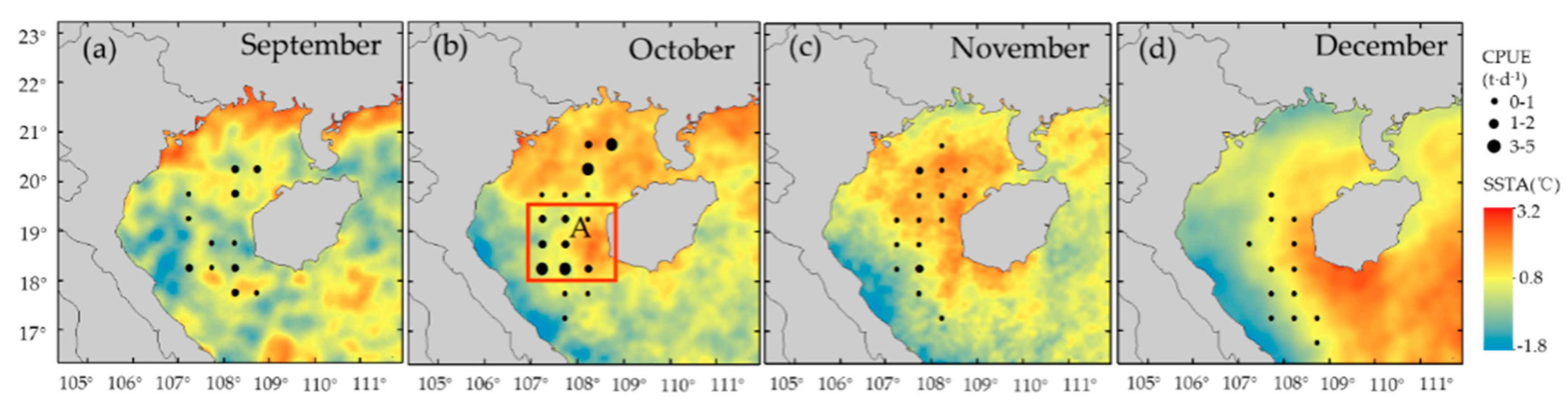
3.1. Relationship between Spatial Distribution of CPUE, SST and NPP

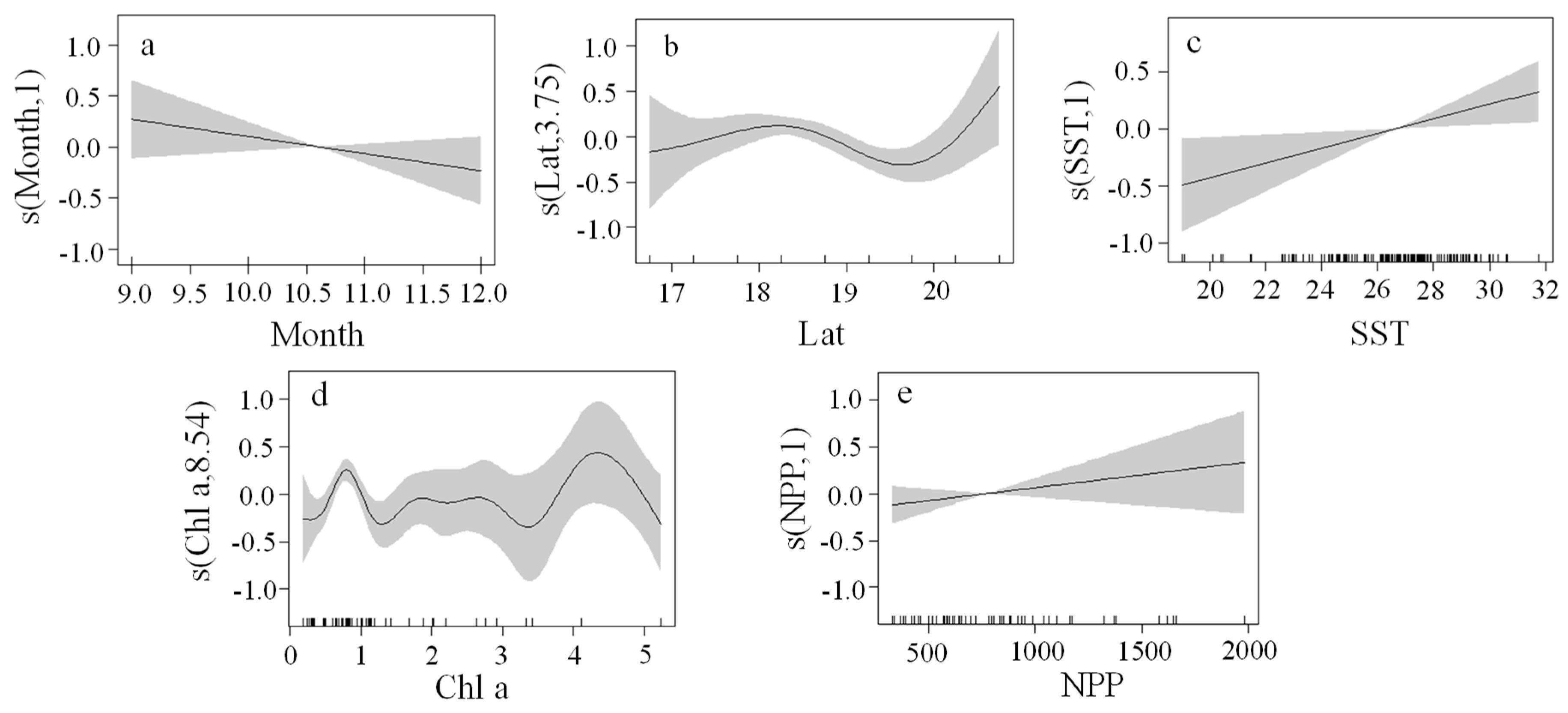
From September to December, as the month increased, SST gradually decreased and changed in the range of 20–30 °C (Figure 2a–d). In October, SST near the Hainan Island (18–19° N) was high, 27–29 °C. From September to December, NPP in the Beibu Gulf increased from 300–1500 mg m⁻² d⁻¹ to 500–3500 mg m⁻² d⁻¹. Spatially, NPP inside the gulf was higher than that outside the gulf (Figure 2e–h). From September to December, the CPUE in the Beibu Gulf increased and then decreased, and the highest CPUE 2-5 t d⁻¹ occurred in October (Box A in Figure 2b). Spatially, high CPUE was mainly distributed in waters at a latitude of 18–19° N and 20–21° N (Figure 2).

3.2. GAM Analysis

GAM was used to fit and predict the impact of spatiotemporal and environmental variables on CPUE in the Beibu Gulf (

Table 2. Deviance analysis for general additive models (GAMs) fitted to the CPUE.

Model Factors	AIC	GCV	Adjusted R2	Cumulative Deviance Explained(%)
Log(CPUE + 1) = s(Month)	586.39	1.45	0.19	4.5
Log(CPUE + 1) = s(Month) + s(SST)	569.30	1.30	0.28	28.7
Log(CPUE + 1) = s(Month) + s(SST) + s(Chl a)	567.32	1.29	0.29	34.0
Log(CPUE + 1) = s(Month) + s(SST) + s(Chl a) +s(Lat)	511.71	1.27	0.35	40.6
Log(CPUE + 1) = s(Month) + s(SST) + s(Lat) + s(Chl a)+s(NPP)	506.83	1.26	0.36	42.9

). The spatiotemporal and environmental factors used were month, latitude (Lat), SST, Chl a and NPP. The total contribution of these influencing factors to CPUE was 42.9%, with the R² being 0.36 (Table 2). In GAM, the relative contribution of selected factors represented the influence degree of each factor on CPUE. Among them, the most influential factor was SST, with a relative contribution of 5.4%, followed by Lat, Chl a, month and NPP, with the relative contribution being 25.2%, 19%, 10.4% and 2.3%, respectively. The results of F-test showed that month, Lat, SST, Chl a and NPP were significantly correlated with CPUE (Pr(F) < 0.05). The results of chi-square test indicated the nonparametric smoothing effect of predictor variables. The most significant effect in the nonparametric smoothing was SST.

The relationship between time factor (month) and CPUE showed that from September to December, CPUE gradually decreased as the month increased (Figure 3a). The spatial factor (latitude) had great influence on CPUE. Within the range of 17–18.25° N, CPUE increased as latitude increased, with the confidence interval become smaller and the reliability increased. Within the range of 18.25–19.75° N, CPUE decreased as latitude increased, with the confidence interval and the reliability increased. While at the range of 19.75°–20.75° N, CPUE increased as latitude increased, and the confidence interval became larger and the reliability decreased (Figure 3b).

Among the environmental factors (SST, Chl a and NPP), SST was the most important influencing factor, and the deviance explained by GAM increased significantly after SST was added to the model. As CPUE increased, SST increased. Within the range of 20–27 °C, the confidence interval decreased gradually, and the confidence level increased. At 27–32 °C, the confidence interval gradually increased and the confidence level decreased (Figure 3c). When Chl a was in the range of 0–0.7 mg m⁻³, CPUE increased as Chl a increased, the confidence interval decreased and the confidence level increased. When Chl a was in the range of 1.3–5 mg m⁻³, CPUE fluctuated as Chl a increased, the confidence interval increased and confidence level decreased (Figure 3d). NPP was positively correlated with CPUE. When NPP was within 300–1000 mg m⁻² d⁻¹, the confidence interval was small and the confidence level was high; when NPP was in the range of 1000–2000 mg m⁻² d⁻¹, the confidence interval was high and the confidence level was low (Figure 3e).

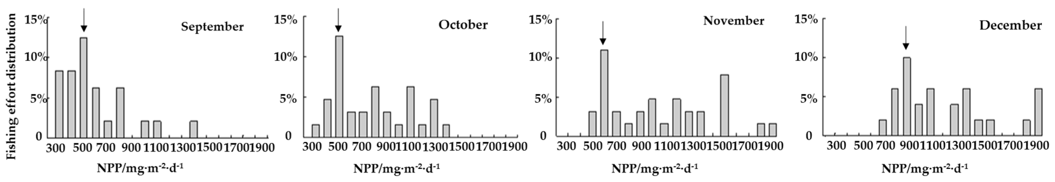
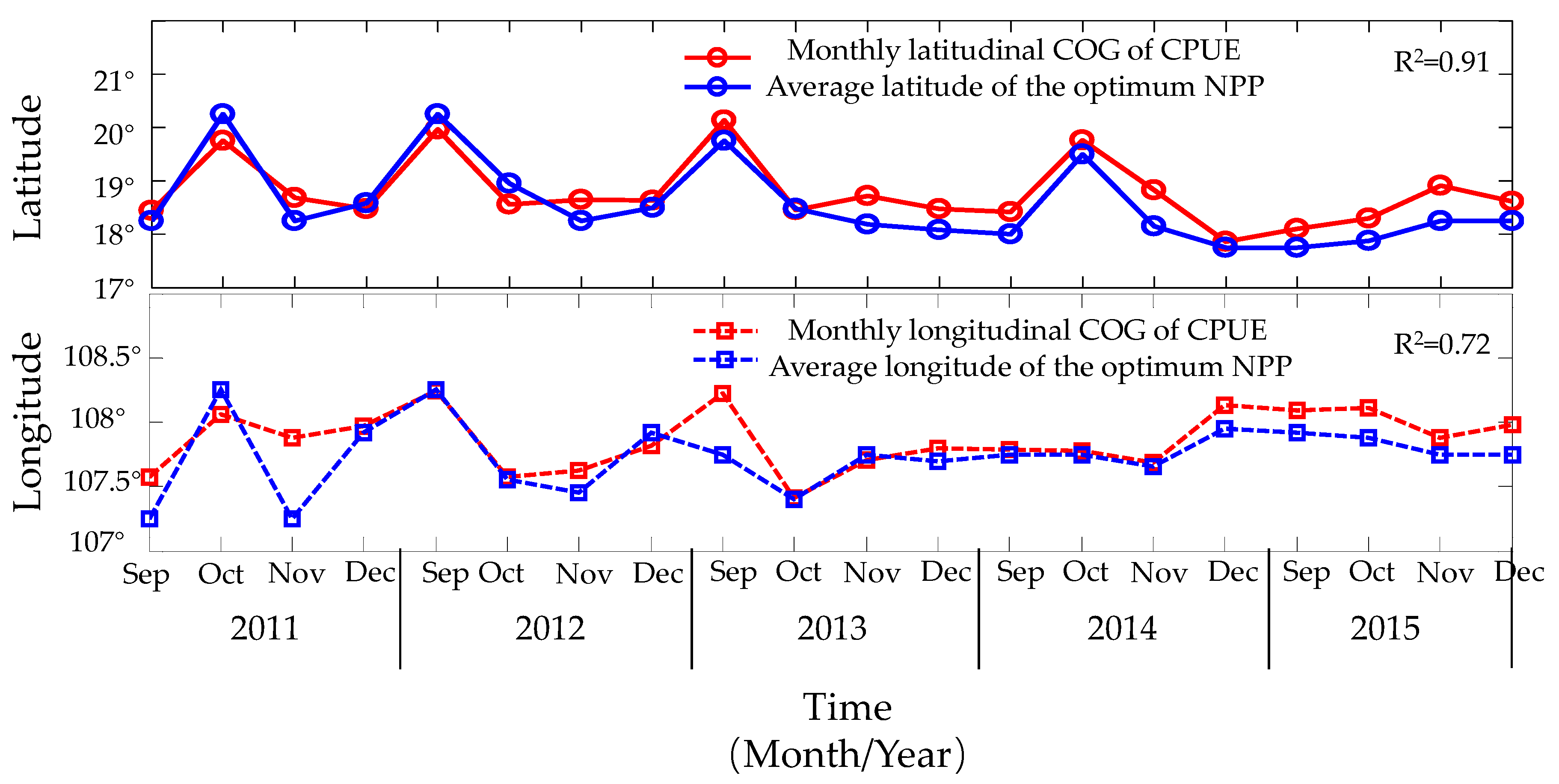
3.3. Relationship between CPUE and NPP

From September to December, CPUE was mainly distributed in waters with NPP of 300–2000 mg m⁻² d⁻¹. The criterion for selecting the suitable NPP for CPUE was that the percentage of operation times accounts for more than 15% of the total operation times of the month [31]. Therefore, the suitable NPP for CPUE from September to December was 300–500 mg m⁻² d⁻¹, 500 mg m⁻² d⁻¹, 600 mg m⁻² d⁻¹ and 900 mg m⁻² d⁻¹, respectively (Figure 4).

From September to December, the longitudinal COG of light falling-net fishing grounds in the Beibu Gulf fluctuated around 107.75° E and the latitudinal COG around 18.5° N. The longitudinal COG was between 107.75–108.25° N, and the latitudinal COG was between 18.5° N and 20–20.25° N (Figure 5). The frequency distribution was used to estimate the relationship between the mean longitude and latitude of the optimum NPP in each month and the longitudinal and latitudinal COG of CPUE. The results showed that the longitudinal and latitudinal COG of CPUE fitted well with the latitudinal COG of the optimum NPP, with a correlation coefficient of 0.91. The longitudinal COG of CPUE fitted well the longitude of the optimum NPP in most months, with a correlation coefficient of 0.72 (Figure 5).

4. Discussion

4.1. Effects of Environmental Factors on CPUE

The relationship between fishery resources and marine environmental factors are complex, nonlinear, and nonadditive [32]. GAM can better demonstrate the nonlinear relationship between dependent and multiple independent variables [33].In this study, we focused on the relationship between environmental factors (SST, Chl a, NPP) and fishery resources in Beibu Gulf. GAM analysis showed that SST had the greatest impact on CPUE of light falling-net fishing grounds in the Beibu Gulf, with a relative contribution of 40%. The catch of light falling-net vessels in the Beibu Gulf includes hairtail, carangidae species and squid, of which hairtail accounts for 45.07% [34]. Hairtail, an omnivorous carnivore, is located in the high nutritional level of marine ecosystem food web. Studies showed that the main feeding targets of hairtail in the Beibu Gulf were carangidae species and squid, and the suitable water temperature was 27–29 °C [35], which was consistent with this study. This water temperature can be one of the indicators of the hairtail habitat. In October, warm pools appeared in the central part of the Beibu Gulf and the western part of the Hainan Island (Figure 2), where the water temperature reached about 28 °C (Figure 2b). The spatial distribution of SST and SSTA were consistent in Beibu Gulf indicated the existence of warm pool (Figure 2 and Figure 6), which helped to reveal the relationship between warm pool and fishery resources. Previous study showed that the development of the warm pool had close relationship with sedimentary, monsoon, upwelling and circulation [36]. The temperature of these warm pools was consistent with that of the most suitable SST for the light falling-net fishing grounds of the Beibu Gulf. The fishery resources in the waters near the warm pools were high (Figure 2b), indicating that the warm pools provided a suitable habitat for fishes to grow. SST, as a good indicator for the distribution of fishing grounds in the Beibu Gulf, can be used as the major environmental factor to forecast the central falling-net fishing grounds in the Beibu Gulf.

The chlorophyll a concentration can reflect the phytoplankton stock in the waters. As an important feeding source of zooplankton, phytoplankton is an important component of the marine’s primary productivity, reflecting the level of primary productivity in the waters [37]. In Beibu Gulf, Chl a was distributed uniformly in most of the bay area, with a belt of higher Chl a along the coast [38]. Nutrient supply from the river discharges is important for phytoplankton growth in the coastal water, but the nutrient up-take from the bottom layer contributes to phytoplankton growth in the center area. Outlier data were deleted before data fusion, in order to remove their influence on GAM. Analysis based on GAM showed that Chl a contributed 19% relatively and NPP contributed 5.4% relatively to CPUE in the Beibu Gulf. The light falling-net fishing grounds in the Beibu Gulf was mainly distributed in waters with Chl a of 0.5–1.3 mg m⁻³ (Figure 3d). In the Taiwan Strait, carangidae fishery were mainly concentrated in waters with Chla of 0.2–1.0 mg m⁻³, which was in consistent with this study [39]. Hairtail in the Beibu Gulf is a high trophic organism with high feeding level. It mainly feeds on cephalopods and crustaceans [35]. The chlorophyll a concentration in the waters directly affects the biomass and distribution of zooplankton, while the distribution of food biomass represented by zooplankton in turn affects the distribution of fishery resources [40]. Previous study showed that the chlorophyll a concentration had a lagging effect to fishery resources [41]. Therefore, the influence of Chl a and NPP on the fishing grounds of the Beibu Gulf are indirect and hysteretic. Chlorophyll a concentration and marine primary productivity play an important role in the marine food chain, as their biomass determines the size of food biomass, and further affects the abundance of fishery resources.

4.2. Spatial Variability of Fishing Grounds

GAM analysis showed that CPUE was mainly concentrated in waters at a latitude of 18.5° N and 20–20.25° N, which was consistent with the COG variation trend of the fishing grounds (Figure 5). Considering the small longitude span of fishing grounds, the interpretative rate of longitude to the model was reduced during the modelling process. Therefore, the longitude factor was not added into the model. The relative contribution rate of latitude to the model was 25.2%. On the one hand, SST of the Beibu Gulf in autumn and winter varied greatly in latitude. SST of the warm pool suitable for fish habitat was 27–29 °C, which was concentrated in waters at a latitude of 18°–19° N [34]. On the other hand, Chl a and NPP in the northern, central and southern parts of the Beibu Gulf differed greatly [10,42]. As a result, the influence of latitude on the distribution of fishery resources in the Beibu Gulf reflected the spatial distribution of environmental factors. From October to December, the northeast monsoon in the Beibu Gulf strengthened, causing local upwelling which drove bottom nutrients to the surface [43,44]. This increased surface Chl a concentration near 18.5° N. The relatively high temperature produced by warm pools and the high nutrients water brought by upwelling provided favorable conditions for fish habitat, leading to the high stock density in October at the latitude of 18.5° N in the Beibu Gulf. In the coastal waters at a latitude of 20–20.25° N, the input of mass terrigenous materials and the intensified tidal mixing [45] brought sufficient nutrients in the waters where phytoplankton were propagated in large quantities, which was conducive to the feeding and aggregation of marine organisms. Therefore, CPUE of fishery resources was high in waters at a latitude of 18.5° N and 20–20.25° N.

4.3. Influence of the optimum NPP on CPUE

Marine primary productivity plays a significant role on marine ecosystem, reflecting the potential yields of marine fisheries [46]. Through the food chain, the variation of primary productivity may determine the change of biological resource population at each trophic level [47,48]. Major catch in the Beibu Gulf were hairtail, carangidae species and squid. Hairtails generally feed on carangidae species and squid, while decapterus maruadsi and squid on zooplankton and small fish [32,49,50,51]. Marine primary productivity determined the food biomass of zooplankton such as decapterus maruadsi and squid [52]. Therefore, from the perspective of feeding level, NPP ultimately determined the stock density in the Beibu Gulf. Relevant studies showed that the optimum NPP of squid fishing ground in the Northwest Pacific was between 500–700 mg m⁻² d⁻¹ from September to November, which was consistent with this study [53]. From July to September, the optimum NPP of mackerel fishing ground in the East China Sea was between 300–500 mg m⁻² d⁻¹, which was slightly different from that in this study [46]. This may be due to the latitudinal difference of fishing grounds, leading to the difference in fishery habitat and further affected the adaptability of fish to the habitat. In addition, there was a significant correlation between the mean latitude of the optimum NPP and the longitudinal and latitudinal COG of CPUE, especially the latitudinal COG, with a correlation coefficient of 0.91 (Figure 5). This indicated that the spatial distribution of CPUE in the Beibu Gulf was subject to the distribution of the optimum NPP, and the optimum NPP could indicate the distribution of central fishing grounds in the Beibu Gulf.

5. Conclusions

The relationship between the spatiotemporal distribution of light falling-net fishing grounds and marine environment of the Beibu Gulf was analyzed using the survey data and satellite remote sensing data. SST was the most important environmental factor affecting the stock density in the Beibu Gulf, with a contribution of 24.2%. Fishing grounds were mainly concentrated in waters at a latitude of 18.5° N and 20–20.25° N, and the mean latitude of the optimum NPP was significantly correlated with the latitudinal COG of CPUE. In this study, we only considered the influence of SST, Chl a, NPP obtained by satellite remote sensing to fishing grounds were analyzed. In the follow-up study, the influence of fishing vessels, salinity, water depth, dissolved oxygen and the interaction between variables on the light falling-net fishing grounds will be considered to improve the accuracy of the model, for effective conservation of fishery habitat in the Beibu Gulf.

References

1. Aoyama, T. The South China Sea Fisheries. The Demersal Fish Stocks and Fisheries of the South China Sea. IPFC South China Sea Fisheries Development and Coordinating Programme; FAO United Nations: Rome, Italy, 1973. [Google Scholar]
2. Cai, Y.C.; Xu, S.N.; Chen, Z.Z.; Xu, Y.W.; Jiang, Y.E.; Yang, C.P. Current status of community structure and diversity of fishery resources in offshore northern South China Sea. South China Fish. Sci. 2018, 14, 10–18. [Google Scholar] [CrossRef]
3. Geng, P.; Zhang, K.; Chen, Z.Z.; Xu, Y.W.; Sun, M.S. Interannual change in biological traits and exploitation rate of Decapterus maruadsi in Beibu Gulf. South China Fish. Sci. 2018, 14, 1–9. [Google Scholar] [CrossRef]
4. Sun, D.R.; Lin, Z.J. Variations of major commercial fish stocks and strategies for fishery management in Beibu Gulf. J. Trop. Oceanogr. 2004, 23, 62–68. [Google Scholar]
5. Wang, X.; Qiu, Y.; Du, F.; Lin, Z.; Sun, D.; Huang, S. Population parameters and dynamic pool models of commercial fishes in the Beibu Gulf, northern South China Sea. Chin. J. Oceanol. Limnol. 2012, 30, 105–117. [Google Scholar]
6. Wang, X.H.; Qiu, Y.S.; Du, F.Y.; Lin, Z.J.; Sun, D.R.; Huang, S.L. Dynamics of demersal fish species diversity and biomass of dominant species in autumn in the Beibu Gulf, northwestern South China Sea. ACTA Ecol. Sin. 2012, 32, 333–342. [Google Scholar] [CrossRef] [Green Version]
7. Ya, H.Z.; Gao, J.S.; Dong, D.X. Analysis of variation characteristics and driving factors of sea surface temperature in Beibu Gulf. Guangxi Sci. 2015, 22, 260–265. [Google Scholar] [CrossRef]
8. Wang, J.Y.; Fang, G.H.; Wang, Y.G. Trends and interannual variability of the South China sea surface winds, surface height and surface temperature in the recent decade. Adv. Mar. Sci. 2017, 35, 159–175. [Google Scholar] [CrossRef]
9. Bauer, A.; Waniek, J.J. Factors affecting chlorophyll a concentration in the central Beibu Gulf, South China Sea. Mar. Ecol. Prog. Ser. 2013, 474, 67–88. [Google Scholar]
10. Shen, C.; Yan, Y.; Zhao, H.; Pan, J.T.; Devlin, A. Influence of monsoonal winds on chlorophyll-α distribution in the Beibu Gulf. PLoS ONE 2018, 13, e0191051. [Google Scholar] [CrossRef] [Green Version]
11. Hastie, T.J.; Tibshirani, R.J. Generalized Additive Models; Chapman and Hall: London, UK, 1990; pp. 587–602. [Google Scholar]
12. Niu, M.X.; Li, X.S.; Xu, Y.C. Effects of spatiotemporal and environmental factors on the fishing ground of Trachurus murphyi in Southeast Pacific Ocean based on generalized additive model. Chin. J. Appl. Ecol. 2010, 21, 1049–1055. [Google Scholar] [CrossRef]
13. Murase, H.; Nagashima, H.; Yonezaki, S.; Matsukura, R.; Kitakado, T. Application of a generalized additive model (GAM) to reveal relationships between environmental factors and distributions of pelagic fish and krill: A case study in Sendai Bay, Japan. ICES J. Mar. Sci. 2009, 66, 1417–1424. [Google Scholar]
14. Wu, J.H.; Dai, L.B.; Dai, X.J.; Tian, S.Q.; Liu, J.; Chen, J.H.; Wang, X.F.; Wang, X.Q. Comparative performance of generalized additive model and boosted regression tree in predicting fish community diversity index in the Yangtze River Estuary, China. Chin. J. Appl. Ecol. 2019, 30, 644–652. [Google Scholar]
15. Solanki, H.U.; Bhatpuria, D.; Chauhan, P. Applications of generalized additive model (GAM) to satellite-derived variables and fishery data for prediction of fishery resources distributions in the Arabian Sea. Geocarto Int. 2017, 32, 30–43. [Google Scholar] [CrossRef]
16. Yu, J.; Hu, Q.W.; Yuan, H.R.; Chen, P.M. Effect assessment of summer fishing moratorium in Daya Bay based on remote sensing data. South China Fish. Sci. 2018, 14, 1–9. [Google Scholar]
17. Siswanto, E.; Ishizaka, J.; Yokouchi, K. Optimal primary production model and parameterization in the eastern East China Sea. J. Oceanogr. 2006, 62, 361–372. [Google Scholar] [CrossRef]
18. Yu, J.; Tang, D.L.; Yao, L.J.; Chen, P.M.; Jia, X.P.; Li, C.H. Long-term Water Temperature Variations in Daya Bay, China Using Satellite and In Situ Observations. Terr. Atmos. Ocean. Sci. 2010, 21, 393–399. [Google Scholar] [CrossRef] [Green Version]
19. Fu, D.; Tang, D.; Levy, G. The impacts of 2008 snowstorm in China on the ecological environments in the northern South China Sea. Geomat. Nat. Hazards Risk 2017, 23, 214–231. [Google Scholar] [CrossRef]
20. R Core Team. R: A Language and Environmental for Statistical Computing; R Foundation for Statistical Computing: Vienna, Austria, 2018. [Google Scholar]
21. Wood, S. Generalized Additive Models: An Introduction with R; Chapman Hall/CRC; CRC Press: Boca Raton, FL, USA, 2006. [Google Scholar]
22. Wood, S.N. Stable and efficient multiple smoothing parameter estimation for generalized additive models. J. Am. Stat. Assoc. 2004, 99, 673–686. [Google Scholar] [CrossRef] [Green Version]
23. Wood, S.N. Fast stable restricted maximum likelihood and marginal likelihood estimation of semiparametric generalized linear models. J. R. Stat. Soc. 2011, 73, 3–36. [Google Scholar] [CrossRef]
24. Gavaris, S. Use of a multiplicative model to estimate catch rate and effort from commercial data. Can. J. Fish. Aquat. Sci. 1980, 37, 2272–2275. [Google Scholar] [CrossRef]
25. Ver Hoef, J.M.; Boveng, P.L. Quasi-poisson vs. Negative binomial regression: How should we model over dispersed count data. Ecology 2007, 88, 2766–2772. [Google Scholar] [CrossRef] [Green Version]
26. Bacha, M.; Jeyid, M.A.; Vantrepotte, V.; Dessailly, D.; Amara, R. Environmental effects on the spatio-temporal patterns of abundance and distribution of sardina pilchardus and sardinella off the mauritanian coast (north-west Africa). Fish. Oceanogr. 2017, 26, 282–298. [Google Scholar] [CrossRef]
27. Venables, W.N.; Dichmont, C.M. GLMs, GAMs and GLMMs: An overview of theory for applications in fisheries research. Fish. Res. 2004, 70, 315–333. [Google Scholar] [CrossRef]
28. Hilborn, R.; Mangel, M. The Ecological Detective: Confronting Models with Data; Princeton University Press: Princeton, NJ, USA, 1997. [Google Scholar]
29. Quinn, T.J.; Deriso, R.B. Quantitative Fish Dynamics; Oxford University Press: Oxford, UK, 1999. [Google Scholar]
30. Wang, J.T.; Chen, X.J. Changes and Prediction of the Fishing Ground Gravity of Skipjack (KatsuwonusPelamis) in Western-Central Pacific; Periodical of Ocean University of China: Qingdao, China, 2013. [Google Scholar]
31. Guo, A.; YU, W.; Chen, X.J.; Qian, W.G.; Li, Y.S. Relationship between spatio-temporal distribution of chub mackerel Scomber japonicus and net primary production in the coastal waters of China. Haiyang Xuebao 2018, 40, 44–54. [Google Scholar] [CrossRef]
32. Stenseth, N.C.; Mysterud, A.; Ottersen, G.; Hurrell, J.W.; Chan, K.; Lima, M. Ecological effects of climate fluctuations. Science 2002, 297, 1292–1296. [Google Scholar] [PubMed] [Green Version]
33. Guisan, A.; Edwards, T.C.; Hastie, T. Generalized linear and generalized additive models in studies of species distributions: Setting the scene. Ecol. Model. 2002, 157, 89–100. [Google Scholar] [CrossRef] [Green Version]
34. Wang, Y.F.; Yu, J.; Chen, P.M.; Yu, J.; Liu, Z.N. Relationship between spatial-temporal distribution of light falling-net fishing ground and marine environments. J. Trop. Oceanogr. 2019, 38, 68–76. [Google Scholar] [CrossRef]
35. Yan, Y.R.; Chen, J.L.; Hou, G.; Lu, H.S.; Jin, X.S. Feeding habits of Trichiurus lepturus in Beibu Gulf of South China Sea. Chin. J. Appl. Ecol. 2010, 21, 749–755. [Google Scholar] [CrossRef]
36. Huang, X.Q.; Cui, Z.A.; Liang, K.; Gan, H.Y.; Xia, Z.; Huo, Z.H. The primary sedimentary characteristics of Warm Pool in Beibu Gulf and its environmental indication. J. Trop. Oceanogr. 2018, 37, 72–89. [Google Scholar] [CrossRef]
37. Yu, J.; Hu, Q.; Tang, D.; Zhao, H.; Chen, P.; Munderloh, U.G. Response of Sthenoteuthis oualaniensis to marine environmental changes in the north-central South China Sea based on satellite and in situ observations. PLoS ONE 2019, 14, e0211474. [Google Scholar] [CrossRef] [Green Version]
38. Tang, D.L.; Kawamura, H.; Lee, M.A.; Dien, V.T. Seasonal and spatial distribution of Chlorophyll-a concentrations and water conditions in the Gulf of Tonkin, South China Sea. Remote Sens. Environ. 2003, 85, 475–483. [Google Scholar] [CrossRef]
39. Li, X.D. Monthly Variability in the Catchability of Chub Macherel and Round Scad and Its Relationship with Environmental Seasonality in the Southern Taiwan Strait; Xiamen University: Xiamen, China, 2006. [Google Scholar]
40. Yu, J.; Hu, Q.; Tang, D.; Chen, P. Environmental effects on the spatiotemporal variability of purpleback flying squid in Xisha-Zhongsha waters, South China Sea. Mar. Ecol. Prog. 2019, 623, 25–37. [Google Scholar] [CrossRef]
41. Yu, J.; Hu, Q.; Li, C.H.; Zhang, P.; Mao, J.M. Relationship between the Symplectoteuthis oualaniensis resource and environmental factors in the Xisha-Zhongsha waters in spring. Haiyang Xuebao 2017, 39, 62–73. [Google Scholar] [CrossRef]
42. Wu, Y.C. The Temporal and Spatial Patterns and Size-Fractioned Structure of Primary Productivity in Beibu Gulf; Xiamen University: Xiamen, China, 2008. [Google Scholar]
43. Lü, X.; Qiao, F.; Wang, G.; Xia, C.; Yuan, Y. Upwelling off the west coast of Hainan Island in summer: Its detection and mechanisms. Geophys. Res. Lett. 2008, 35, 196–199. [Google Scholar] [CrossRef]
44. Zhang, S.P.; Wang, J.; Zhao, H. Influence of monsoon on temperal-spatial distribution of particulate inorganic carbon concentration time in the Beibu Gulf. J. Guangdong Ocean. Univ. 2015, 35, 78–86. [Google Scholar] [CrossRef]
45. Song, X.Y.; Huang, L.M.; Shi, Y.R. Progress in research on primary production of esturies and bays. Ecol. Sci. 2004, 23, 265–269. [Google Scholar] [CrossRef]
46. Guan, W.J.; Chen, X.J.; Gao, F.; Li, G. Study on the dynamics of biomass of chub mackerel based on ocean net primary production on southern East China Sea. ACTA Ecol. Sin. 2013, 35, 121–127. [Google Scholar] [CrossRef]
47. Keenan, T.F.; Hollinger, D.Y.; Bohrer, G.; Dragoni, D.; Munger, J.W.; Schmid, H.P.; Richardson, A.D. Increase in forest water-use efficiency as atmospheric carbon dioxide concentrations rise. Nature 2013, 499, 324–327. [Google Scholar] [CrossRef]
48. Chassot, E.; Melin, F.; Pape, O.L.; Gascuel, D. Bottom-up control regulates fisheries production at the scale of eco-regions in European seas. Mar. Ecol. Prog. 2007, 343, 45–55. [Google Scholar] [CrossRef] [Green Version]
49. Wang, Y.X. Fishery biological characteristics of swordtip squid Loligo edulis in the southern part of the East China Sea. Mar. Fish. 2002, 24, 169–172. [Google Scholar] [CrossRef]
50. Jiang, R.J.; Xu, H.X.; Jin, H.W.; Zhou, Y.D.; He, Z.T. Feeding habits of blue mackerel scad Decapterus maruadsi Temminck et Schlegel in the East China Sea. J. Fish. China 2012, 36, 216–227. [Google Scholar] [CrossRef]
51. Huang, M.Z. Feeding habits of Decafterus maruadsi in Taiwan Strait. J. Oceanogr. Taiwan Strait 1995, 14, 399–406. [Google Scholar]
52. Xu, Z.L.; Cui, X.S.; Huang, H.L. Distribution of zooplankton in Ommastrephes batramii fishing ground of the North Pacific Ocean and its relationship with the fishing ground. J. Fish. China 2004, 28, 515–521. [Google Scholar] [CrossRef]
53. Yu, W.; Chen, X.J.; Yi, Q. Relationship between spatio-temporal dynamics of neon flying squid Ommastrephes bartramii and net primary production in the northwest Pacific Ocean. Haiyang Xuebao 2016, 38, 66–74. [Google Scholar] [CrossRef]
Figure 1. Research area and survey stations.
Jmse 08 00957 g001
Figure 2. Spatial distribution of sea surface temperature (SST), net primary production (NPP) and catch per unit effort (CPUE) in the Beibu Gulf: (a) SST in September, (b) SST in October, (c) SST in November, (d) SST in December, (e) NPP in September, (f) NPP in October, (g) NPP in November, (h) NPP in December.
Jmse 08 00957 g002
Figure 3. GAM analysis of the effects of the spatiotemporal and environmental factors on CPUE in the Beibu Gulf: (a) month, (b) latitude (lat), (c) SST, (d) chlorophyll a concentration (Chl a) and (e) NPP. Shadow areas, 95% confidence intervals. Rug plots on the x-axis, relative density of data points.
Jmse 08 00957 g003
Figure 4. Relationship between the percentage of operation times and NPP in the fishing grounds of the Beibu Gulf from September to December.
Jmse 08 00957 g004
Figure 5. Relationship between the center of gravity (COG) of fishing grounds and the optimum NPP in the Beibu Gulf.
Jmse 08 00957 g005
Figure 6. Spatial distribution of SST anomaly (SSTA) in Beibu Gulf: (a) SSTA in September, (b) SSTA in October, (c) SSTA in November and (d) SSTA in December.
Jmse 08 00957 g006