1. Introduction
Storms, together with tides, are the main driving force for coastal flooding events that have impacted coastal zones throughout history. For example, the years of 1953 and 1962 were marked by strong storm surge events, which, combined with tides, caused flooding over broad coastal areas in the south-western Netherlands and eastern England [
1], and in northern Germany [
2], respectively. In the last decade, the Xynthia (27 to 28 February 2010) storm severely impacted low-lying coastal areas located in the central part of the Bay of Biscay [
3,
4,
5,
6], causing 53 fatalities and material damage assessed at more than one billion euros. This event was a mid-latitude storm resulting in a storm surge of about 1.5 m, which coincided with a spring high tide. These examples illustrate the potentially devastating effect that storm surges can have on the coasts and the need for a better prediction of storm surge phenomena.
Nearshore storm surge is mainly a consequence of atmospheric surges and wave setup [
4,
7]. Atmospheric surges result from the direct effect of wind (especially in shallow-water) and atmospheric pressure (both in shallow and deep water), while the breaking of waves generates the wave setup. The theoretical model of the inverse barometer (IB) is the simplest way to estimate the storm surge. This approach can be efficient for lands or islands surrounded by deep seas, however, most of the time this is not sufficient, because it does not account for the local and regional effect of the wind [
8], neither for the wave set up contribution [
4,
7]. In addition to the IB approach, there are mainly two types of methods to estimate storm surges: dynamical approaches such as dynamical downscaling (DD) and data-driven approaches such as statistical downscaling (SD). Advantages and disadvantages between DD and SD approaches were discussed for the specific case of waves on the coast of France [
9]. They concluded that there is a balance between representing physical processes and statistical relationships; the first are limited by computational time and resources, the latter are faster but have a limited ability to explain all the physical processes.
The DD relies on the use of numerical models solving physical equations, for instance, the shallow-water equations. Generally, DD allows a good representation of physical processes with a high resolution both in time and space; however, they need data for boundary and forcing conditions (e.g., observed or regional model outputs for wave parameters, water level, tidal constituents, wind magnitude, and direction, see for instance [
4]) and the simulations can demand a high computational effort [
10,
11]. In addition, precise local modeling requires the availability of good bathymetric data and sometimes complex modeling techniques. For instance, if the wave setup is expected to play a significant role, then the numerical modeling should rely on two coupled models: one focusing on the atmospheric storm surge, most of the time using shallow-water equation models, and another focusing on waves and the resulting wave setup using a spectral wave model [
4,
7].
The SD establishes a statistical link between the predictor (e.g., averaged regional atmospheric data such as sea level pressure, SLP) and the predictand (e.g., measured or simulated storm surge or wave parameters for a given point). SD approaches present good approximations in terms of the statistical distribution of the variable to be predicted with few input variables, but usually have limitations when applied to short-term predictions (e.g., minutes and hours) and extreme events [
12,
13,
14,
15,
16]. For example, an SD method based on a multiple linear regression linking principal components of atmospheric data to local modeled atmospheric surge levels was used to reconstruct historical daily maximum storm surge (SS) on a global scale from 1871 to 2010 [
14]; and also applied for the specific case of southeast Asia [
15] and New Zealand [
16].
Another example of an SD method is the weather-type approach, which has been widely used for estimating wave parameters as well as storm surge and wave parameters combined. This technique has been mainly used to investigate climate-related variability and future projections, analyzing monthly and annual distributions [
9,
17,
18,
19]. In these studies, the principal components of the predictor are clustered, resulting in different groups of data, called weather types (WT). An improvement of this method is the weather type regression guided approach [
12]. It works as the former method, but, in the clustering process, information on the predictand is included in addition to the predictor variable (SLP and sea level pressure gradient (SLPG)) through a weighting scheme (via an α factor).
Other SD methods that rely on machine learning algorithms have been applied for the estimation of storm surge. For instance, the artificial neural network algorithm has been used for short-term local predictions associated with severe storms, such as hurricanes [
20,
21,
22,
23,
24,
25,
26], as well as for the study of extreme events on a global scale [
27]. The random forest algorithm has also been used for the estimation of global SS and compared with DD approaches, showing that data-driven methods can perform equally or better on storm surge predictions than dynamical models on a global and long-term scale [
28].
Although the SD models were applied to a large range of locations around the world with good efficiency, the predictions for enclosed seas and bays, where the geographical settings can play an important role, are sometimes not as satisfactory as for exposed coastlines, especially for maximum value daily predictions [
12,
14,
16,
18,
19]. Another limitation is that despite the fact the multiple linear regression approach presents good approximations for daily predictions [
14,
15,
16], it does not establish an easy visualization and direct link between the WTs and local storm surge response; while the SD weather types approach can do it, but is not originally designed for daily predictions. The design of SD models based on the WT approach requires the defining of several key elements, which can vary accordingly to the study site, spatial-temporal scale, and target variable of the prediction (in this manuscript, SS). Some of these elements are the weather type’s selection method and the configuration of the predictor, by setting the appropriate variable and spatial-temporal domain.
The present study aims to: (1) build a WT-based method to set up a statistical downscaling model to estimate the daily maximum value of storm surge, and (2) estimate the added value in comparison with other models. For this development, we focus on predicting the storm surges at the La Rochelle–La Pallice tide gauge (France). For instance, we will show how our SD model can provide valuable information on the atmospheric patterns of storms responsible for the extreme daily values of local storm surges.
2. Study Site and Database
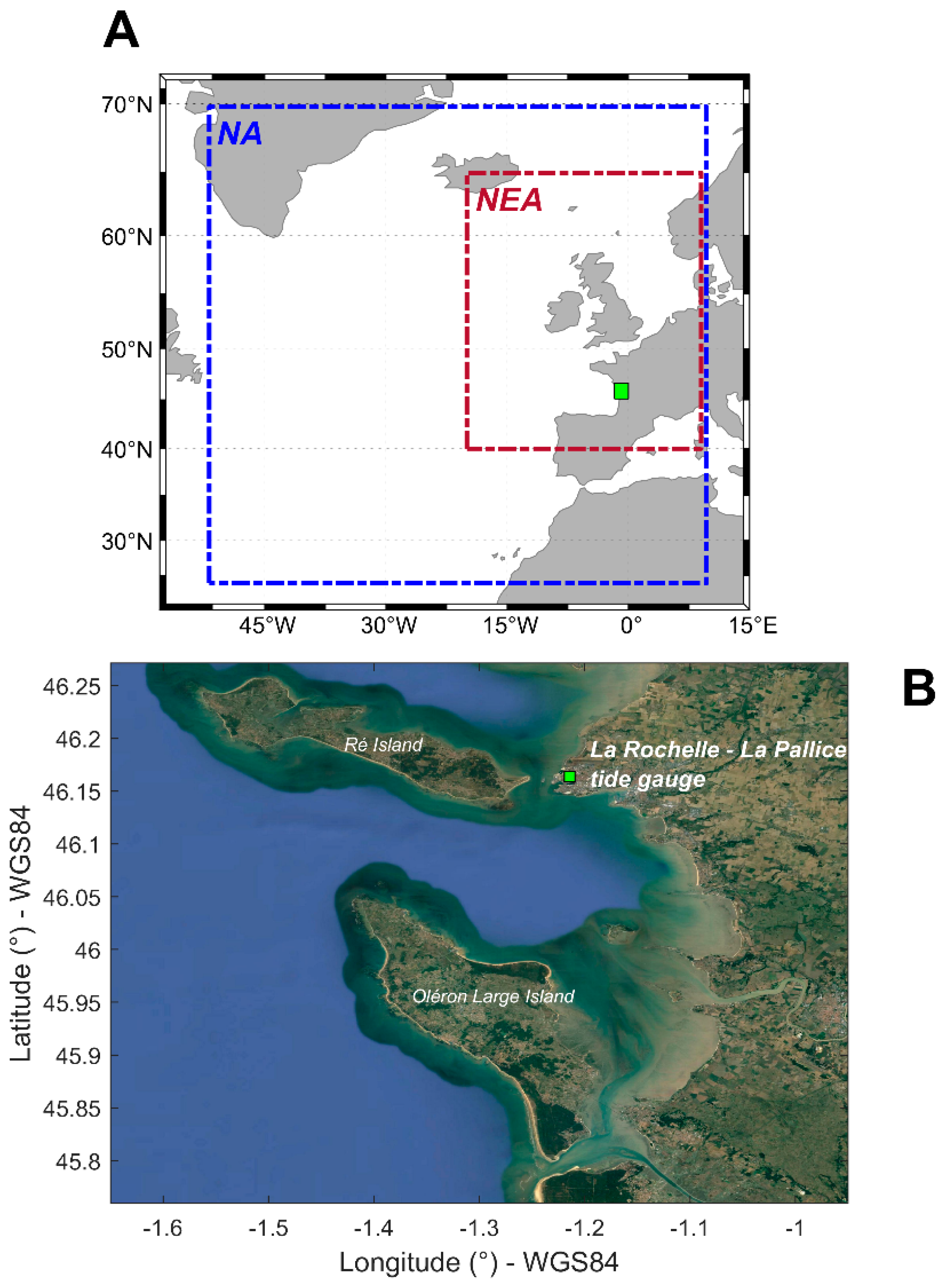
La Rochelle is located along the south-west coast of France, New Aquitaine, in the maritime region called the Bay of Biscay, as shown in
Figure 1. It is located at the inner shelf, protected by swells due to the presence of Ile de Ré and Ile d’Oléron. This implies that the average and extreme events of storm surges (e.g., Xynthia, 2010) that occurred in this area do not result only from the inverse barometric effect, but also from the wind effect and regional wave setup [
3,
4]. The choice of La Rochelle as our study site aims at ensuring a minimum level of complexity in the surge signal. There is one tidal gauge (La Rochelle–La Pallice) and a weather station, operated by SHOM (Service Hydrographique et Océanographique de la Marine) and Météo-France, respectively.
To set up our statistical models, which aim to predict SS for La Rochelle–La Pallice, we need to define a predictor and predictand data (see
Section 3.1 and
Section 3.2 for more details). For the predictor definition process, we use the atmospheric CFSR and CFSRv2 reanalysis data [
29,
30,
31] over the 1979 to 2014 period. These datasets have a spatial resolution of 0.33° and 0.22°. Here, we used the following hourly output data: sea level pressure (SLP), wind magnitude (WND), and geopotential height at 500 hPa (GP). In addition, to investigate the effect of the spatial domain of the predictor, these variables were extracted onto the domain of the North Atlantic (NA) and northeast Atlantic (NEA) zones,
Figure 1A.
The predictand data is derived from the water level measured at La Rochelle–La Pallice (available at
data.shom.fr, tidal gauge station doi: 10.17183/REFMAR#34). First, the observed storm surge dataset is estimated by subtracting the predicted tide provided by the SHOMAR software [
32] to the water level measurements, resulting in a time-series covering the period from 1941 to 2014. Due to the many data gaps in the records before 2000, we focus on the 2000 to 2014 period, for more reliable results. Thus, the time-series is post-processed to extract the maximum storm surge per day (i.e., SS), defining the predictand data.
Figure 2 presents the respective dataset, showing extreme storm surges exceeding 1 m, with the largest value (~1.5 m) observed on 28 February 2010, corresponding to the Xynthia event.
This outstanding storm has unique aspects. According to previous numerical modeling work [
3], the unusual trajectory from SW to NE enables the storm to produce short waves that significantly enhanced the atmospheric storm surge at La Rochelle–La Pallice, which represented about 94% of the Xynthia storm surge, the rest being induced by the regional wave setup [
4]. This proportion depends on the characteristics of the storm. For instance, for the Joachim storm (15 to 16 December 2011), the relative contribution of the atmospheric storm surge to the surge was smaller (88%) (deduced from the results of [
4]), highlighting the non-negligible effect of the regional wave setup on surges in such environments.
3. Methods
Here, we first give a general explanation of the statistical downscaling weather type approach (
Section 3.1). Second, we describe the sensitivity tests made (e.g., on predictors selection, clustering technique) to identify the optimal configuration for the proposed SD (
Section 3.2). Third, we describe the alternative predictive models (e.g., formers SD multiple linear regression and SD WT models) whose performances are compared with the optimal model resulting from set-up sensitivity tests (
Section 3.3).
3.1. A Generalized Explanation of the Weather Type Approach
As already introduced (
Section 1), the statistical downscaling weather types approach is based on the establishment of a statistical relationship between regional atmospheric data, i.e., predictor, and local response of a given marine variable (e.g., wave parameter and/or storm surge) which is the target of study, i.e., predictand.
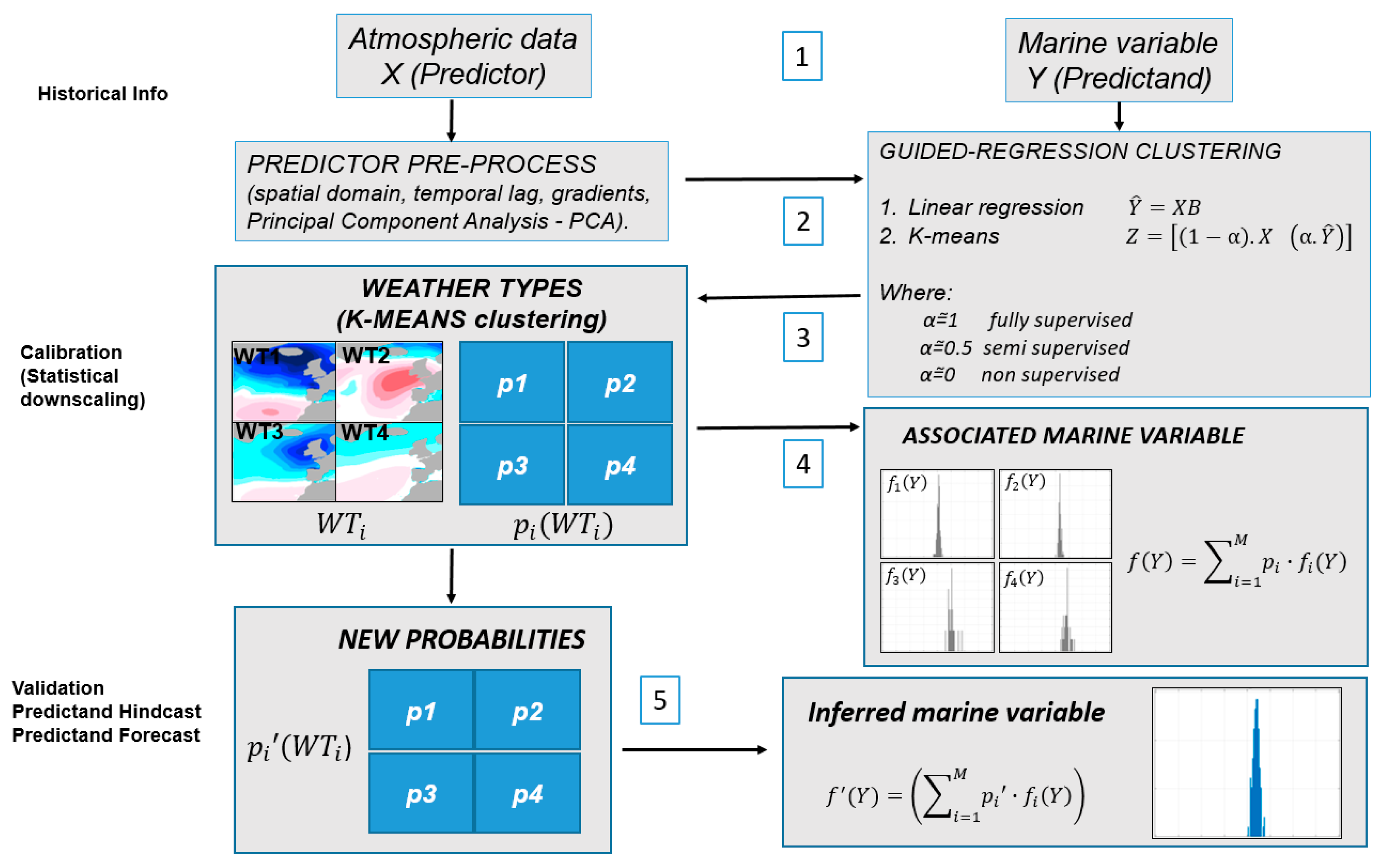
Figure 3 illustrates the main steps. The arrows and numbers indicate the flow and steps of the method, respectively. This figure is a generalization of the WT approaches applied for the wave climate prediction [
13], and combined wave and storm surge climate [
12]. In what follows, we detail each step, based on these past studies, while the application of this general framework to SS prediction is detailed in
Section 3.2 and
Section 4.1.
Accordingly, with [
12] this method is composed of the following steps: (1) collecting of historical data for the predictor and predictand followed by pre-processing; (2) performing a regression-guided classification (first, a multiple linear regression between predictand and predictor, and second, a classification of the predictor and the estimations of the predictand); (3) defining the weather types of the synoptic circulation conditions; (4) establishing the statistical relationship between predictor and predictand (empirical distribution functions of SS are calculated for each WT); (5) validating the statistical model or applying the model to different temporal periods.
First, the pre-processing of predictor and predictand historical data need to be executed. For the European Atlantic coast, former works [
14,
16,
20] used as predictors variables SLP and SLPG fields covering an area from 20° to 80° N and from 60° W to 50° E of the North Atlantic basin; while the predictand data used were daily mean wave parameters and storm surge. The predictor’s domain area was defined by the evaluation of source and travel time of wave energy reaching a local area (ESTELA) method, which shows that for the most part, the wave energy that reaches the European coast takes three days to travel from the genesis point [
33,
34].
Then, for the cases of wave climate prediction [
12,
13], the predictor is defined as the three-day mean SLP and three-day mean SLPG, calculated every day through the historical time period. Thus, the predictor associated with a certain day corresponds to the average obtained using the same day and the previous two days. This process aims to reduce the dimensionality of the data and also takes into account the time response between the atmospheric system and the consequent storm surge. A principal components analysis (PCA) is applied to the predictor in order to reduce the dimensionality of the data and simplify the classification process. From all the principal components (PCs) identified, just the ones which together explain 95% of the data variance are selected [
13].
Second, the regression-guided classification is performed. To start with, a multivariate regression between predictors PCs and predictand daily data is developed, resulting in predicted marine variables. The predicted data is then concatenated with the PCs in a new matrix, structured just as shown in
Figure 3, step 2 (for details on this procedure see [
12]). Thus a K-means algorithm (KMA) is applied to the concatenated matrix (step 3), dividing the data space into a number of clusters, each one defined by a prototype and formed by the data for which the prototype is the closest [
35]. The number of clusters should be pre-defined, which is 100 in former studies applying this approach for the North Atlantic region [
12,
13]. The maximum-dissimilarity algorithm (MDA) is performed to initiate the prototypes, which guarantees a deterministic classification and the most representative initial subset. The level of influence between atmospheric and marine variables (predictor and predictand, respectively) in the classification is controlled by a weighting factor α [
36]. In the case α = 0, an unsupervised multivariate regression classification is applied; for α = ~0.5, a semi-supervised multivariate regression-guided classification is applied; and for α = 1, a fully supervised classification is performed.
Still, in the third step, the WTs are calculated as the mean of the synoptic circulation conditions (i.e., cluster center) included in each cluster of the regression-guided classification. The statistical relationship between the predictor and the predictand is established in the fourth step: the empirical probability distributions of daily local marine variables are calculated for each WT (f
i), following the equation in
Figure 3, step 4, considering the probabilities (p) of each WT and their associated distribution during a given calibration period. In the fifth step, given a validation period, the predictand is predicted where p
i is the probability of the WT in the validation period (WT
i).
3.2. Procedure for Identifying the Best SD Using WT Approach Configuration
In order to set up a statistical downscaling model of SS for La Rochelle–La Pallice tidal gauge station, we follow the general procedure (
Figure 3) and first perform sensitivity tests to identify the best configuration of the model (called SD1). The tests are done by varying each parameter presented in
Table 1, one at a time.
To evaluate the influence of different spatial domains of weather patterns, two predictor domains were used (
Figure 1): the North Atlantic (NA) and northeast Atlantic (NEA). Indeed, modeling experiments suggest that the atmospheric storm surges at La Rochelle are driven by the NEA meteorological patterns [
5,
37], while the regional wave setup is related to swells whose generation domain extends to the NA domain [
4]. The spatial resolution of the predictor is another important factor in the downscaling technique. Thus, the CFRS (0.33°) and CFRSv2 (0.22°) data were linearly interpolated at three different resolutions (0.5°, 1°, 2°) in the predictor’s domain.
There is a time lag between the atmospheric condition and its local storm surge response, which can vary on a scale of days [
12,
13,
34]. As explained in
Section 3.1, this is taken into account by calculating the X-day average predictor variable, calculated every day through the historical time period. Thus, the predictor associated with a certain day corresponds to the average obtained using the same day and the previous n days (X-day average = (certain day + n days)/(n + 1)). We tested X = 2, 3, and 4 day-average as the predictor variable.
In order to determine the weather types, a clustering technique is applied. For this purpose, we tested the usual KMA approach and the so-called self-organizing maps (SOM) [
38]. For evaluating the effect of semi-supervised versus fully supervised classification on model performance, α parameter values of 0.2, 0.6, 0.8, and 1 were tested. In all the cases tested, a number of 100 clusters was pre-determined to start the clustering algorithm based on former studies using the WT approach for the North Atlantic region [
12,
13].
Regarding the predictor variables, the most common approach is to use SLP and SLPG. However, other atmospheric variables could be considered as relevant predictors for storm surges like wind magnitude at 10 m above the sea surface (WND) and the geopotential height of the 500 hPa (GP). Thus, we investigated the following predictor variables: daily minimum SLP and daily maximum SLPG; daily minimum SLP and daily maximum WND; daily mean GP; daily maximum GP.
The model performances are evaluated in terms of root mean squared error (
, Equation (1), with
n number of days), maximum absolute error (
, Equation (2)), and r-squared (
, Equation (3)), compared with the observed SS. The error indicators are calculated for every year and also averaged over the five years of the validation period (
) and described as follows:
Thus, for each configuration,
Table 1, the model is calibrated using 14-year-long data from the 15-year dataset (2000 to 2014). The remaining one-year-long period is used for validation purposes, following a leave-one-year-out cross-validation. This procedure is done for five individual years (
K = 2010 to 2014).
3.3. Comparing the Best Model Configuration with Former Models
With the aim to compare the performance of the optimal model (SD1,
Section 3.2 and
Section 4.1) with the alternative prediction methods based on former approaches, several tests were performed (see
Table 2). For all the tests, we keep a spatial resolution of 1° in the NA domain and use the same validation procedure as in
Section 3.2.
The SD2 is a statistical downscaling model based on multiple linear regression [
14]. It does not estimate the statistical relation between classified weather types and the daily maximum surge level (SS) but, instead, directly fits a multiple linear regression model between PCs of the atmospheric predictor and SS. Thus, the daily maximum surge level at a given location (xi) holds as follows:
where
pn is the number of PCs of atmospheric data that explains 95% of the variance,
ai,
b1,i,
bn,i are the coefficients obtained in the regression model. As the predictor, SD2 uses the two-day mean of daily mean SLP and SLPG.
The SD3 and SD4 are weather type statistical downscaling methods based on semi [
12] and non-supervised classification [
13], focused on combined wave and storm surge climate and on wave climate predictions, respectively (see
Figure 3, step 2). Here, these methods are adjusted to predict the SS: the daily maximum observed storm surge is set as the predictand variable instead of the daily average of wave parameters. As the predictor, SD3 and SD4 use the two-day mean of daily mean SLP and SLPG.
The IB model (for inverse barometer) is based on the relation between local pressure variations (∆P
A in units) around the mean atmospheric pressure (
) over the oceans and the local changes in sea-level (∆ζ), expressed by Equation (5), where ρ is the salt-water density (kg/m
3) and g is the acceleration of gravity (9.8 m/s
2).
In the present study, the analysis of the local measurements at the meteorological station in La Rochelle (Meteo France), provides a mean sea level pressure ( = 1017 hPa).
Finally, it is important to remark that the comparison between the SD1 model and the alternatives should not be seen as an absolute statement, but only as an estimation of the method skills for predicting SS, on a site like La Rochelle–La Pallice.
4. Results
The results are described in the subsections below. First (
Section 4.1), we present the results regarding the comparison between different configurations of the SD using WT approach, following the procedure explained in
Section 3.2. Second (
Section 4.2), the best model’s configuration is compared with former models as described in
Section 3.3. Third (
Section 4.3), we compare the different WT classifications performed by the optimal configuration and other WT based models (SD3 and SD4).
4.1. Comparing Different SD Based on WT Approach Configurations
The results of the sensitivity tests for different model set-ups for the five validation years (K = 2010 to 2014) are summarized in
Figure 4, in terms of
. Similar results are reached by considering the other performance criteria (
Table A1). Each arch refers to a parameter tested, which was varied one at a time with respect to the SD1 configuration (identified as the optimal model). Several observations can be made.
First, the use of the North Atlantic domain (NA) shows better results (i.e., lower MAE) than the northeast Atlantic domain (NEA). This highlights the importance of large-scale patterns in the atmospheric predictor, since the NA domain does not only include the area of the atmospheric surge genesis but also the swell generation zone which produces the regional wave-setup in the surrounding of La Rochelle.
The 1° resolution has the best performance, showing that the relation between the error and the spatial resolution is not monotonic: the highest resolution (0.5°) leads to the largest error values (
= 0.09;
= 0.57 m;
= 0.69); and similarly, the coarser resolution (2°) performs poorly (
= 0.08;
= 0.50 m;
0.77), as can be observed in
Figure 4 and
Table 1A in
Appendix A.
One possible explanation is that the increase in the predictor dimensionality can worsen the performance of the clustering step, i.e., the identification of the WTs. This relies on the fact that PCA is applied in this method to reduce the dimensionality of the dataset by removing redundant data in means of variance in the spatial and temporal domain (e.g., strongly correlated data), thus allowing the clustering algorithm to improve its performance. The predictor dimensionality is 1364, 5580, and 21,894 for the 2°, 1°, and 0.5° spatial resolutions, respectively, which are transformed to 64, 82, and 98 PCs, which explains 95% of the data variance. This shows that a higher resolution requires more PCs to explain the same percentage data variability and that predictor dimensionality increases with spatial resolution, but this does not imply better model performance. Indeed, for too high resolution, there could remain too much redundant data (“noise”), while, for too low resolution, the variability may not be sufficiently captured. Thus, there should be an optimal resolution for properly describing the variance, but avoiding too much redundant data. In addition, we should highlight that the local predictand (storm surge) is a response to the atmospheric conditions but also to local bathymetry and coastal morphology. These local processes are not related to the synoptic circulation. Therefore, the introduction of more detailed information about the atmospheric conditions does not necessarily improve the skill of the downscaling method. Regarding the number of days used to define the predictor, the model performance is improved by using the two-day average. This last aspect will be discussed in more detail in
Section 5.
Concerning the clustering process, the use of the KMA algorithm shows a better capability than SOM to predict the daily maximum surge (further discussion in
Section 5). Furthermore, the fully supervised regression guided classification (α = 1) shows an outstanding improvement of the predictions, principally in terms of
, when α increases,
decreases to 0.41 m (α = 1). The other error metrics exhibit similar behavior, with
(
) decreasing (increasing) as α values increase (leading to
= 0.07 and
= 0.78 for α = 1).
Finally, the combination of the two-day mean daily minimum SLP and two-day mean daily maximum SLPG as predictors leads to the best surge predictions in La Rochelle. By using these predictors, we account for both the intensity of the storms and their dynamics. This builds a more heterogeneous dataset for the clustering process. This ensures the identification of the extreme weather patterns responsible for the maximum storm surge at the coast.
4.2. Performance Comparison with Alternative Prediction Approaches
The overall performance of the tested models is estimated by analyzing
and
(the averaged RMSE and MAE errors for the five validation years 2010 to 2014), as shown in
Figure 5. SD1 exhibits the best results (
~0.07 m and
= ~0.4 m). Although SD2 exhibits a similar
, it presents a worse
(~0.55 m). SD3 shows similar results compared with SD2, while SD4 and IB models exhibit the worst performances.
To better illustrate the models’ performances, we analyze the different validation years separately. For example,
Figure 6 presents the results (observed and modeled SS time series, scatter plot, and errors) for the 2010 validation year, which contains the maximum observed storm surge value of ~1.5 m (Xynthia storm, 28 February 2010). For each model, the MAE corresponds to the error in predicting the Xynthia SS. The optimal model (SD1) has the best fit with the measured data in terms of RMSE = 0.07 m, MAE = 0.5 m and R
2 = 0.8. The multiple linear regression model (SD2) also shows a good approximation with similar values of RMSE (0.09 m) and R
2 (0.7), but with a worse value of MAE (1.08 m), corresponding to a 58 cm larger underestimation of the Xynthia SS. This reinforces that using extreme daily predictor values (i.e., min SLP and max SLPG), with a fully supervised regression guided clustering, can improve the prediction performance, in particular of the upper tail of the predicted data distribution, i.e., rare and extreme events.
The inverse barometer model (IB) provides the worst results, as expected since this model only computes the local variations in sea level pressure, ignoring the action of regional weather patterns, wind stress, and waves. The SD4 model provides a better approximation than IB by including regional atmospheric patterns, but it is not capable of properly representing the distribution of SS since the weather pattern and predictand data are not directly linked statistically during the clustering step (i.e., non-supervised classification). This is improved in the SD3 as this model clusters a concatenated matrix composed of weather patterns (PCs) and predictand data, by applying a semi-supervised classification (see
Figure 3, step 3).
4.3. Weather Types and Storm Surges in La Rochelle
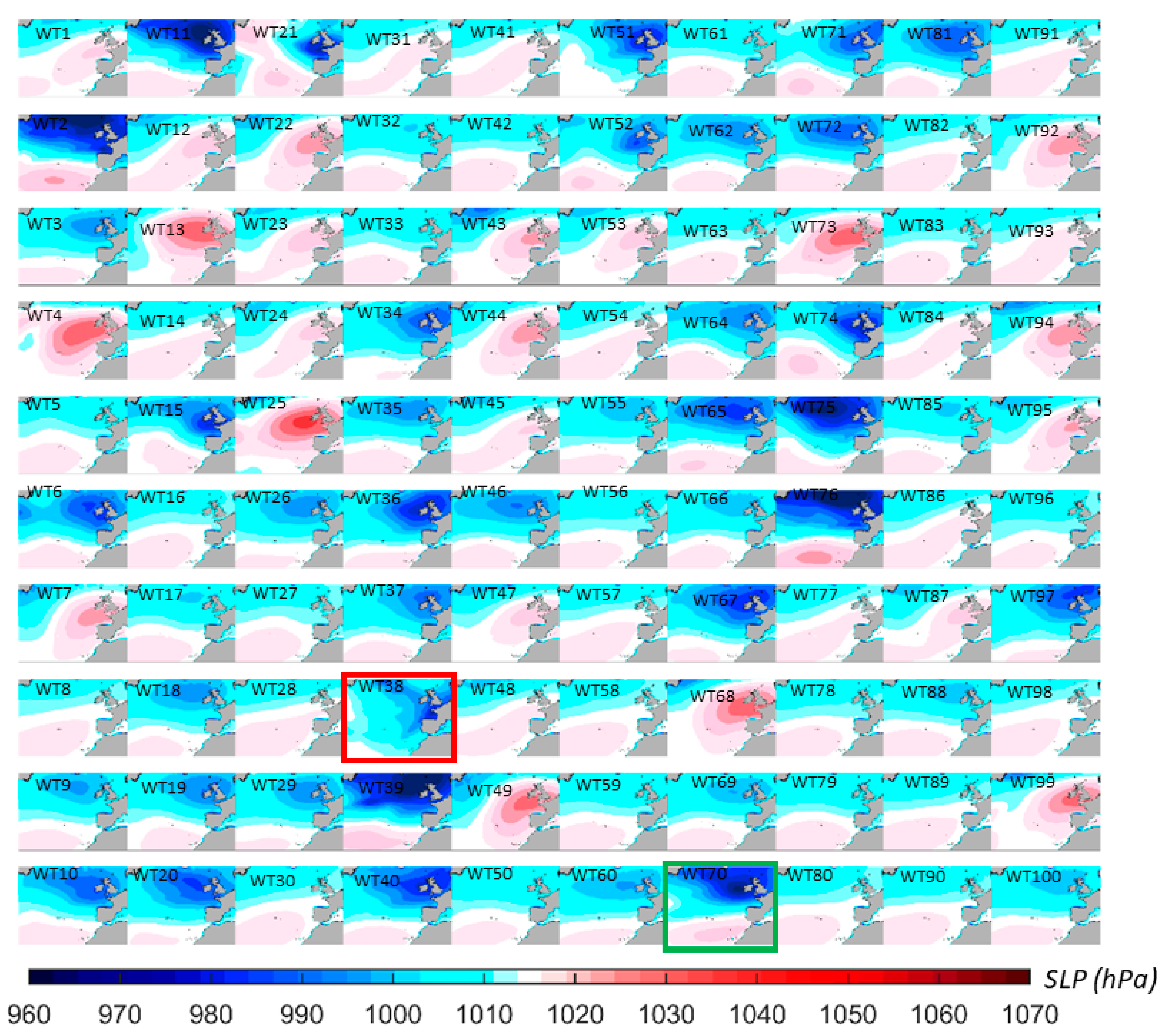
The use of a fully supervised regression guided classification in the SD1 model has shown good performance in identifying both regional and local synoptic patterns associated with average and extreme events of storm surge at La Rochelle. This is illustrated in
Figure 7, which shows the daily minimum SLP fields associated with each of the 100 weather types classified during the calibration period from the years 2000 to 2014 and validation period K = 2012. As observed, most of the WTs are associated with positive surge daily maximum values, while few others have negative surge values distributions, corresponding to the action of the high-pressure areas. It should be noted that the Xynthia and Joachim storms fall in the weather types WT38 (red rectangle) and WT70 (green rectangle), respectively.
The atmospheric regional patterns can be identified as patterns that spread all over the domain and, in some cases, exhibit centers of low and high pressure clearly defined by an accentuated SLP gradient (e.g., WT2, WT11). On the other hand, there are patterns not so well defined (e.g., WT41, WT86), which are usually related to more frequent events, and lower atmospheric gradient. Regarding the local synoptic patterns, they can be easily recognized by the accentuated gradients and centers of low and high sea level pressure covering an area from the United Kingdom to the Bay of Biscay including the English Channel (e.g., WT51, WT25).
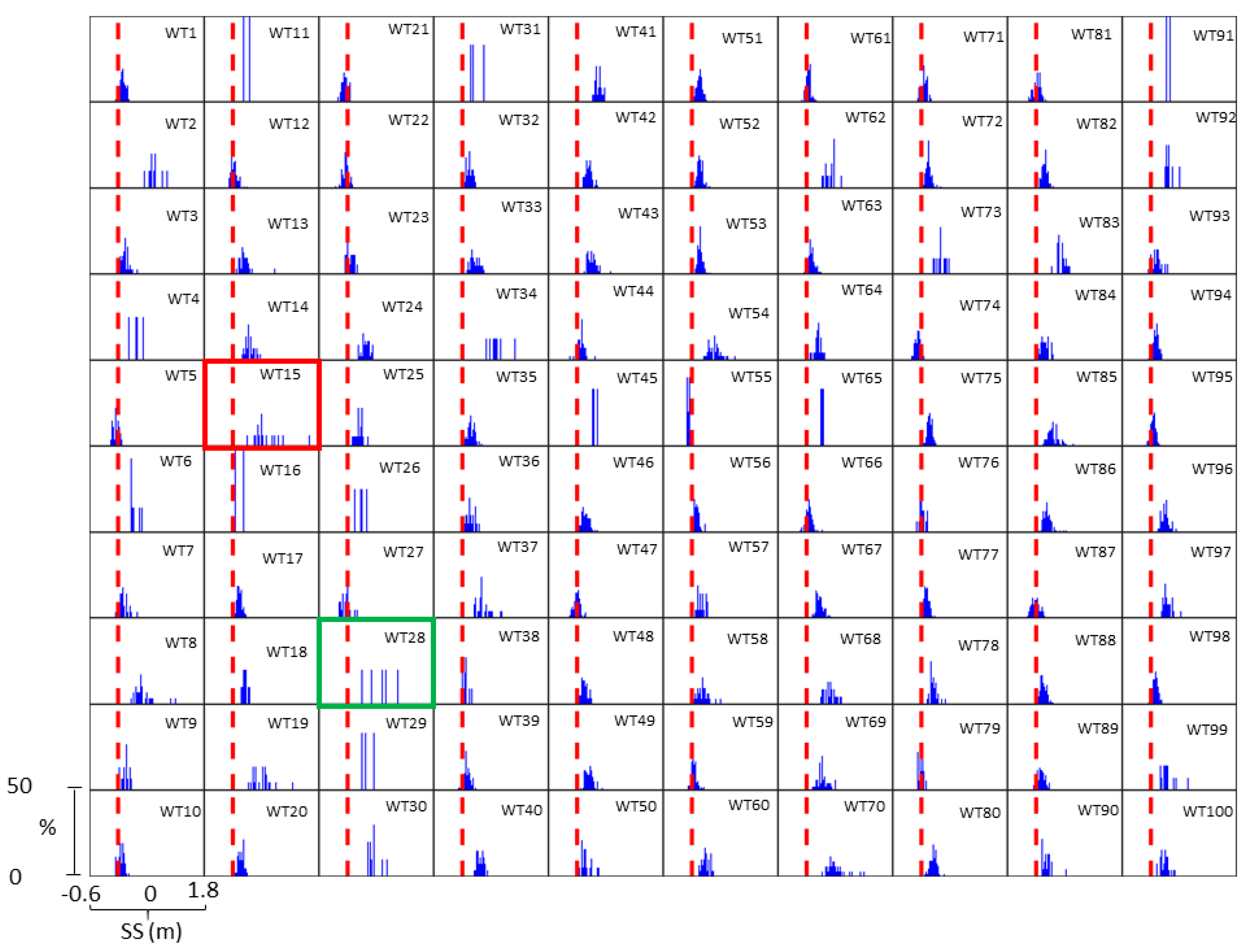
Observing
Figure 8, which shows the SS distribution associated with the corresponding WT, it can be seen that the highest storm surge values are linked with low-frequency weather types, with regional (WT75, WT76) and local patterns (WT6, WT21). Sometimes these WTs occur only once over the whole calibration period as in the case of the Xynthia storm (2010), represented by WT38 which looks like a local storm. Note that the Joachim (2011) storm is also well represented by WT70, showing a regional scale weather pattern, which highlights the model’s capability to recognize both regional and local extreme storms.
This recognition is lost when compared with the WTs identified by SD3 and SD4 models, based on the semi-supervised and non-guided regression classification approaches, respectively (see
Section 4.2 and
Appendix A,
Figure A1,
Figure A2,
Figure A3 and
Figure A4). In these cases, only the regional weather patterns are identified, such that the model has a lower performance in classifying extreme events like Xynthia and Joachim as unique or rare events. Instead, these storms are classified as part of other WT, with ordinary surge responses, leading to an underestimated prediction.


