Component Velocities and Turbulence Intensities within Ship Twin-Propeller Jet Using CFD and ADV

Abstract

This study presents the decays of three components of velocity for a ship twin-propeller jet associated with turbulence intensities using the Acoustic Doppler Velocimetry (ADV) measurement and computational fluid dynamics (CFD) methods. Previous research has shown that a single-propeller jet consists of a zone of flow establishment and a zone of established flow. Twin-propeller jets are more complex than single-propeller jets, and can be divided into zones with four peaks, two peaks, and one peak. The axial velocity distribution is the main contributor and can be predicted using the Gaussian normal distribution. The axial velocity decay is described by linear equations using the maximum axial velocity in the efflux plane. The tangential and radial velocity decays show linear and nonlinear distributions in different zones. The turbulence intensity increases locally in the critical position of the noninterference zone and the interference zone. The current research converts the axial momentum theory of a single propeller into twin-propeller jet theory with a series of equations used to predict the overall twin-propeller jet structure.

1. Introduction

A propeller ejects water backward from the ship in a rotating motion to provide the reacting forces to drive the ship forward. The ejected water is known as a propeller jet. The initial plain water jet was studied by Albertson et al. using the axial momentum theory [1]. This was converted as the theoretical basis for the propeller jet. Hamill [2] measured the internal flow of a single-propeller jet according to the physical model. Lam et al. [3] reported that the tangential velocity of a six-bladed propeller is lower than that of a three-bladed propeller, and Lam [4] summarized previous studies on ship single-propeller jets. Numerical simulations and physical tests have been conducted for comparison with the prediction equations for the propeller jet. The velocity distribution and turbulence intensity distribution of the ship propeller jet have been revealed, sparking interest in propeller jet research. Guo et al. [5] investigated the hydrodynamic characteristics of a marine propeller operating in oblique inflow using the CFD method. Huang et al. [6] presented a numerical method for predicting the effective wake profile of a high-speed underwater jet. Prabhu et al. [7] calculated the flow characteristics around propeller blades using the panel method. The boundary layer was used to estimate the effect of viscosity on the flow. Ohashi [8], Zhang et al. [9], Abramowicz-Gerigk and Gerigk [10], Wu et al. [11], and others have enriched the research on the hydrodynamic forces around the propeller.

A twin-propeller system is suitable for large vessels that need a more powerful thrust than a single propeller can provide. The independent flow field of the two propellers is disturbed due to the relatively small distance between the two propellers. Jiang et al. [12] presented a jet structure induced by a twin propeller. The two jets developed independently near the propeller, but the two flow fields were mixed as a result of the jet diffusion. The velocity on the seabed induced by a twin-propeller ship without a rudder was investigated and compared with previous theoretical expressions by Mujal-Colilles et al. [13]. The prediction equations for ship propeller jet velocity proposed in previous studies and the current study are shown in Appendix A.

2. Methodology

ANSYS Fluent 15.0 (ANSYS 15.0 Fluent Users Guide) [14] was used to run a numerical simulation associated with geometry creation using SOLIDWORKS 2016 (SOLIDWORKS Tutorials) and meshing using ICEM 15.0 (ANSYS ICEM CFD User Manual 15.0).

2.1. Propeller Characteristics

Many types of propellers are used in ships. Propeller characteristics are usually defined by the blade number, propeller diameter, thrust coefficient, pitch ratio, cross profile of the blade, and other parameters. Two single-propeller models with diameters of 131 mm and 76 mm were selected in the current investigation according to the Ph.D. study of Lam [15]. The characteristics of Propeller-131 and Propeller-76 are presented in

Table 1. Propeller characteristics.

Properties	Twin-Propeller-131	Twin-Propeller-76
Diameter of propeller, $D_p$	131 mm	76 mm
Diameter of hub, $D_h$	35 mm	14.92 mm
Pitch ratio, $P^{\prime }$	1.14	1
Rake angle, $\mathsf{\theta }$	0°	0°
Blade number, N	6	3
Thrust coefficient, $C_t$	0.56	0.4
Distance from hub to hub, $L_h$	2 × 131 = 262 mm	2 × 76 = 152 mm
Blade area ratio, $\mathsf{\beta }$	0.922	0.473

. For the current investigation, the distance between the rotating axes of the 2 propellers must be defined. The hub spacing of twin propellers has a great influence on the jet structure. At present, the setting of hub spacing of twin-propeller slurry is applied from 1.5-times of diameter to several-times of diameter. Taking a twin-propeller cargo ship as an example, it has a length of 80 m, width of 16.5 m, propeller diameter of 3.2 m, and hub spacing of 6.8 m. For the common small- and medium-sized transport vessels, the spacing of 2-times the diameter is widely used. In this study, the distance of 2$D_p$ was used as the research object. Figure 1 shows the propellers used in the subsequent numerical simulation.

The thrust coefficient $C_t$ is a dimensionless coefficient determined by the performance characteristics of the propeller and is related to the disk ratio of the propeller. The thrust coefficient can be obtained from the open water characteristic curve of propeller.

2.2. Computational Fluid Dynamics (CFD) Numerical Simulation

The current investigation used ICEM 15.0 software for grid generation. Lam [15] suggested that the grid for the water subdomain could be meshed by the structure grid for more calculation accuracy. The rotor subdomain is suitable for an unstructured grid. The meshed twin-propeller system and surrounding fluid are shown in Figure 2. The propeller plane is intercepted from the computational domain grid of propeller-76. The mesh generation of rotation domain and propeller rotor is shown in Figure 2a. The mesh division of propeller-131 is shown in Figure 2b.

In this study, the calculation domain was set as a cuboid domain. The upstream length was 2$D_p$, and the downstream length was 50$D_p$. The width of the cross-section rectangle was 14$D_p$ and the length was 16$D_p$. According to the requirements for the grid model of the rotating reference frame, the entire computing domain was divided into 4 regions: An upstream domain, rotation domain, ring rotation domain, and downstream domain. The diameter and length of the 2 cylindrical rotating domains containing the 2 propellers was 1.2$D_p$ and 1$D_p$, respectively.

A structured grid and an unstructured grid were used in the modeling. For the complex geometry of the rotation domain, it was difficult to create a structured mesh, and the mesh quality was low due to high torsion. Thus, unstructured meshes were used in the 2 rotation domains. For the simple geometry of the upstream basin, ring rotation domain, and downstream basin, a more accurate and controllable structured grid was used. The upstream and downstream basins were divided into single O-type grids. The ring rotation domain was divided into 2 O-shaped meshes on the left and right sides. Each region was connected by an interface. The mesh size ratio on both sides was less than 1.2. The grid density was higher in the region closer to the rotation domain.

The generation of a boundary layer grid has a significant influence on the calculation results. In the CFD calculation, $y^{+}$ is generally used to calculate the height of the grid nodes in the first layer [14], as shown in Equation (1).

$$y^{+}=\frac{y\rho {\mu }_t}{\mu }$$

(1)

The first-layer grid distance calculation is shown in Equation (2).

$$y=L{y}^{+}\sqrt{80}R{e}_L^{-13/14}$$

(2)

where L is the characteristic length and $R{e}_L$ is the Reynolds number.

The number of layers in the boundary layer should satisfy Equation (3).

$$N_{normal}=\{\begin{array}{ll}10& \mathrm{for}\mathrm{wall}\mathrm{function}\\ 15& \mathrm{for}\mathrm{low}-\mathrm{Re}\mathrm{model}\end{array}$$

(3)

According to Equation (2), the height of the first-layer grid of the boundary layer on the surface of the propeller blade was 0.0005 m ($y^{+}$ ≈ 30). The grid was stretched by 10 layers with a tensile rate of 1.1. The total thickness of the boundary layer was 0.013 m. The volume mesh size in the rotation domain was set to 0.003 m.

The inlet was set as the pressure inlet with an incoming velocity of 0 m/s. The outlet boundary condition was set as the pressure outlet. The surfaces of the propeller blade and hub were set as nonslip rotating walls. The other boundaries were set as nonslip walls. Each basin was connected by an interface.

The multiple reference frame model was used for calculation and a steady-state solution was obtained. In the calculation process, relative motion of the grid does not occur and the rotation of the water area replaces the rotation of the propeller. Four different grid sizes (4 mm, 3 mm, 2.5 mm, 2 mm) were used to test the grid independence with $L_h$= 2$D_p$, n = 1000 rpm, and N = 3. When the volume mesh size changed from 3 mm to 2 mm, the number of meshes increased by 77% but the variation was reduced by only 0.29%. The mesh size in the rotation domain was chosen as 3 mm, as shown in

Table 2. Jet outflow velocity at each grid resolution.

Grid Size	Number of Grids in the Rotation Domain	Total Number of Grids	$\mathbf{Jet}\mathbf{Outflow}\mathbf{Velocity}{\mathit{V}}_0$
4	185,430	1,604,586	1.346 m/s
3	267,100	2,098,170	1.344 m/s
2.5	405,040	3,248,520	1.343 m/s
2	566,204	3,646,028	1.348 m/s

. The standard k–ε model was used to ensure the accuracy and convergence of the calculation.

Versteeg and Malalasekera [16] introduced turbulence and its modeling. The standard k–ε turbulence model, with good astringency and accuracy, was chosen for the twin-propeller jet. Lam [15] suggested that a propeller could be defined by a second-order discretization scheme. An independence analysis for the grid ensures that the grid refinement has little influence. The rotation speeds of Twin-propeller-76 and Twin-propeller-131 were 1000 rpm and 350 rpm, respectively, as suggested by Lam [15]. Jiang et al. [12] introduced specific details for setting the numerical simulation of a twin-propeller jet.

2.3. Experiment Setup

In this study, a model experiment was designed to verify the previous theoretical research and numerical simulations of a propeller jet. A water tank, 1.2 m long, 0.8 m wide, and 0.45 m high, was selected to allow the expansion of twin-propeller jets, as in previous studies [17]. The power train system was designed and fabricated from a motor, a gearbox, and connecting rods to allow the twin propeller to rotate outward and inward at different speeds. Acoustic Doppler velocimetry (ADV) was used for the point measurements. A purpose-built traverse system allowed the ADV to accurately measure the scour depth, as shown in Figure 3. The submergence of the propeller affects the jet structure. It is mainly caused by the adhesive force of the boundary. In the experiment, the diameter of the propeller was 55 mm. The water depth of the flume was 400 mm. Small boundary effects could be observed at a distance from the propeller. However, near the propeller, the boundary effect could be ignored. The test measurement was mainly carried out in the boundless influence area.

The structure of the jet and the rudder was affected by the structure of the hull. Researchers have studied the single-propeller jet for decades. The original research method also started from an unlimited propeller. After that, the influence of rudder and other structures was considered. Compared with the high-speed propeller jet, the influence of hull structure is negligible. However, the rudder structure has a great influence on the jet velocity distribution. The study of the twin-propeller jet is still in the initial stage. The influence of ship structures on jet will be gradually considered in later research.

3. Validation

According to Jiang et al. [12], the interference effect of two propeller jets can be ignored at the efflux plane. The thrust (T) of the twin-propeller system is the same as the thrust of a single propeller for model validation. T is defined by Equation (4).

$$\mathrm{T}=C_t\rho n^2{D}_p^4$$

(4)

where T is the propeller thrust, $\rho$ is the density of water, $D_p$ is the propeller diameter (m), and n is the rotation speed.

Substituting the Propeller-76 rated $C_t$ value of 0.4 into Equation (4), the theoretical T value was calculated as 3.71 N. The CFD results indicate that T = 3.6 N for each propeller in the Twin-propeller-76 system. The difference between the theoretical result and the CFD result was 3%. Substituting the Propeller-131 rated $C_t$ value of 0.56 into Equation (4), the theoretical T value was calculated as 5.61 N and the CFD result was 5.21 N. The difference was 7.1%, which may have been due to weakened fluid acceleration resulting from the proximity of the two propellers. The CFD numerical simulation was compared with the measured data and Lam’s data [15] to verify the reliability of the results.

The current CFD numerical simulation of two propeller jets has the same propeller model as the single-propeller jet. Owing to the limitations of the experimental equipment, the size of the propeller model was slightly smaller in the model test. The current study compared the dimensionless axial velocity distribution at 1$D_p$ within ZFE-TP-4P, as shown in Figure 4. The central axes of the two propellers were located at y/Rp = −2 and y/Rp = 2. The dimensionless axial velocity distribution of the experimental measurement and CFD simulation shows four obvious peaks. The mirrored results of Lam [15] were very similar to the experimental results. The largest variation occurred at y/Rp = 2.6, possibly due to measurement errors. The turbulence of the propeller fluctuated greatly. When the ADV measures the velocity at a certain point in the jet, it represents the average velocity for a short period of time. The wake may deviate sufficiently along the axis during the measurement time to produce an error. The nondimensional axial velocity distribution variation within y/Rp > −2.6 was less than 20%. A lower axial velocity occurred on the axis of rotation, approximately 0.5–0.6 V_a/V_max. Between the two propellers, the axial velocity decreased significantly. The minimum value at y/Rp = 0 was approximately 0.1 V_a/V_max. The CFD simulation results show that the dimensionless axial velocity was approximately zero between y/Rp = −1 and y/Rp = 1. The diffusion of the two propeller jets was more obvious in the experimental test than in the CFD simulation.

The jet at the center of the outflow plane was not thrusted by the blade due to the shielding effect at the center hub of the propeller. At the tip of the blade, the jet only underwent a very small acceleration process. Therefore, the wake velocity at the hub and blade tip was small. The fluid in the middle of the blade was accelerated from the leading edge to the trailing edge. The outflow velocity reached the maximum velocity. There were two maximum velocity peaks on the outflow plane of each propeller. The energy of the fluid was exchanged with that of the surrounding fluid in the form of a vortex. For the twin-propeller jet, the initial vortex has two main causes. One is the outward diffusion between the two propeller jets. The other is the inward diffusion between the low-speed core at the hub of a single propeller and the high-speed jet at the blade. This study confirms that, when the latter diffusion is completed, the former continues. A maximum velocity peak (two peaks) was formed at each propeller axis. Finally, the fusion of the two propeller jets was completed to form a single peak area.

Indeed, it was found that the diffusion of the propeller wake was more rapid than that of CFD simulation such that the “Plateau” between the two propellers was not found in the experimental measurement.

Figure 5 shows the distribution of the dimensionless turbulence intensity at 1$D_p$ within ZFE-TP-4P. The CFD simulation shows four peaks near the two propeller axes. However, this was not observed in the experimental records or in Lam’s results [15]. The maximum variation was 52%, which occurred at the axis of the left propeller.

For experimental measurements, the propeller jet was a high-speed turbulence. The jet was not the uniform diffusion state of CFD simulation. In the experiment, it can be observed that the center of the jet of the twin-screw propeller shifted. The offset distance can even be up to twice the diameter range. When measuring the velocity at a certain position of the jet, a large deviation occurred in the time of recording the jet velocity. Therefore, the experimental measurement in Figure 5 has a large variation with CFD results. This measurement variation was more obvious downstream.

4. Velocity Distribution

For the initial plane jet and propeller jet, the velocity of the jet has always been the most important research concern. The velocity of a single-propeller jet has been thoroughly studied by previous researchers. Jiang et al. [12] validated that the jets behind the two propellers are mixed through jet diffusion. The structure of a twin-propeller jet was suggested by CFD simulation and was different from that of a single propeller. However, their research was based on only one representative propeller model. The current Twin-propeller-131 jet was added to compare different propeller-induced jet structures.

4.1. Axial Velocity Distribution

A ship is driven by the counterthrust of the propeller. The driving force is generated mainly by the axial velocity component. The diffusion of the propeller jet is due to the axial velocity, which may also cause problems such as riverbed erosion.

4.1.1. Efflux Velocity

Previous studies originated from the efflux velocity of the propeller. The axial momentum theory provided a theoretical basis for subsequent studies. Inspired by the study of plain water jets by Albertson et al. [1], Stewart [18] proposed that the thrust provided by propellers satisfies Equation (5). The application of the axial momentum theory in the calculation of efflux velocity of a propeller jet is shown in Figure 6. The zone (A) far upstream and zone (D) far downstream are far enough away from the propeller that the fluid pressure (P_A) at zone (A) and the fluid pressure (P_D) at zone (D) are equal to the hydrostatic pressure. When the fluid flows through the propeller, it accelerates from zone (B) to zone (C) through the propeller. Pressure (P_B) increases to (P_C). The velocity also increases from $U_B$ to $U_C$.

$$\mathrm{T}=\frac{1}{2}\rho A_p\left(U_D^2-U_A^2\right)$$

(5)

Equation (4) and Equation (5) can be combined.

$$\frac{1}{2}\rho A_p\left(U_D^2-U_A^2\right)=C_t\rho n^2{D}_p^4$$

(6)

As the advance speed $U_A$ = 0 and the area $A_p=2\mathsf{\pi }{D}_p/4$, Equation (6) becomes

$$\frac{\mathsf{\pi }{D}_p^2}{8}{U}_D^2=C_t{n}^2{D}_p^4$$

(7)

The theoretical result of the efflux velocity can be expressed as Equation (8).

$$U_D=1.59n{D}_p\sqrt{C_t}$$

(8)

In the current CFD model, the speed of the ship was neglected with a still water domain. Hence, Equation (8) can be derived using the axial momentum theory, the most widely used equation for predicting jet efflux velocity. Both $U_D$ and $V_0$ represent the outflow velocity. $U_D$ is the symbolic representation used in the theoretical derivation based on the axial momentum theory and $V_0$ is the common symbol.

For the efflux velocity of the theoretical result calculated by Equation (8), Lam’s [15] and Hamill’s [2] experimental results were compared with the CFD results in

Table 3. Comparison of current study and previous studies on efflux plane.

Source	Equation	Efflux Velocity (m/s)	Variation (%)
Axial momentum theory (Prop-76)	$V_0=1.59n{D}_p\sqrt{C_t}$	1.27	5.2
Lam [15] (Prop-76)	$V_0=1.59n{D}_p\sqrt{C_t}$	1.27	5.2
Hamill [2]	$V_0=1.33n{D}_p\sqrt{C_t}$	1.06	28
Current CFD results (Prop-76)	-	1.34	-
Axial momentum theory (Prop-131)	$V_0=1.59n{D}_p\sqrt{C_t}$	0.91	8.1
Lam [15] (Prop-131)	$V_0=1.59n{D}_p\sqrt{C_t}$	0.91	8.1
Hamill [2]	$V_0=1.33n{D}_p\sqrt{C_t}$	0.76	23
Current CFD results (Prop-131)	-	0.99	-

. For Twin-propeller-76, the theoretical result, Lam’s results [15], and Hamill’s results [2] were 5.2%, 5.2%, and 28% less than the CFD results, respectively. For Twin-propeller-131, they were 8.1%, 8.1%, and 23% less than the CFD results, respectively. The accelerating effect of the twin-propeller system on the incoming flow was more intense than that of the single-propeller system. The CFD results show that the jet velocity of the propeller depends mainly on the size and rotation speed of the propeller and has little relation to the type of propeller.

4.1.2. Position of the Efflux Plane

Previous studies have shown that the velocity distribution on the outflow plane satisfies the Gaussian distribution. The velocity distributions of the two twin-propeller systems were similar. However, the radial distance of the efflux velocity of Twin-propeller-131 occurred at $0.85\left(R_p-R_h\right)$ from the rotation axis, which is further than $0.62\left(R_p-R_h\right)$ for Twin-propeller-76. The axial velocity distribution obtained from the CFD numerical simulation is shown in Figure 7. Lam [15] proposed that the maximum jet velocity is related to the maximum thickness position of the blades. The blade geometry of the two twin propellers shows that the point of maximum blade thickness for Prop-131 is farther from the rotation axis than for Prop-76. As a result, the position of maximum velocity for Twin-propeller-131 was farther from the rotation axis than for Twin-propeller-76, as shown in

Table 4. Positions of maximum efflux velocity.

Source	Equation	Position (mm)	Variation (%)
Berger et al. [19] Stewart [18] McGarvey [20]	$R_{mo}=0.67\left(R_p-R_h\right)$	32.2 (Propeller-131) 20.5 (Propeller-76)	21
Prosser [21]	$R_{mo}=0.6\left(R_p-R_h\right)$	28.8 (Propeller-131) 18.3 (Propeller-76)	29
Hamill [2]	$R_{mo}=0.7\left(R_p-R_h\right)$	33.6 (Propeller-131) 21.4 (Propeller-76)	17
Lam [15]	$R_{mo}=0.83\left(R_p-R_h\right)$ for Propeller-131 $R_{mo}=0.74\left(R_p-R_h\right)$ for Propeller-76	39.8 (Propeller-131) 25.3 (Propeller-76)	2.42.5
Current CFD results	$R_{mo}=0.85\left(R_p-R_h\right)$ $R_{mo}=0.62\left(R_p-R_h\right)$	40.8 (Propeller-131) 26.0 (Propeller-76)	-

.

Lam’s experimental results [15] showed that the efflux velocity of Twin-propeller-131 occurred at $0.83\left(R_p-R_h\right)$, which is 2.4% less than the CFD calculation results, while the efflux velocity of Twin-propeller-76 occurred at $0.74\left(R_p-R_h\right)$, which is 19% greater than the CFD calculation results.

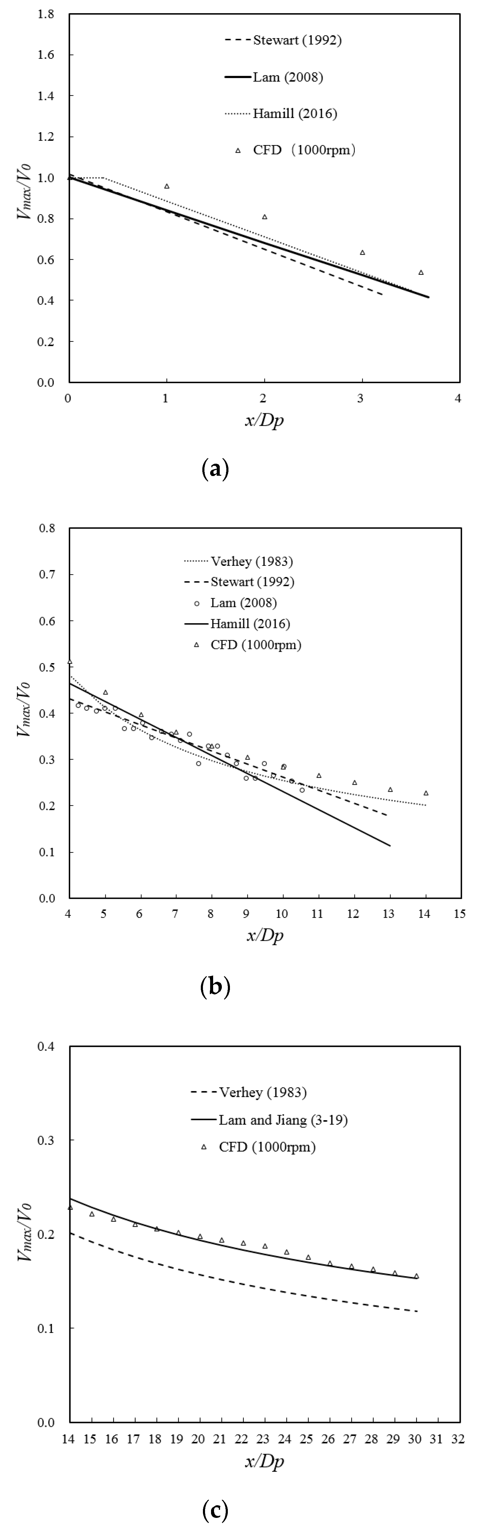
4.1.3. Axial Velocity Decay

Jiang et al. [12] suggested several equations for predicting the twin-propeller jet-induced axial velocity decay according to the CFD results for the Twin-propeller-76 jet. Stewart [18] proposed that the propeller type does not affect the decay of the maximum axial velocity. However, Hamill et al. [22] refuted Stewart’s idea based on an experiment with four different propellers. Hamill et al. [22] showed that different types of propeller jets decay differently. Figure 8 compares the maximum axial velocity decay of Twin-propeller-76 and Twin-propeller-131. The CFD result for axial velocity decay of a twin propeller was greater than Lam’s experimental result [15] for a single propeller. The maximum axial velocity of Twin-propeller-131 decayed more slowly than that of Twin-propeller-76.

The axial velocity decay in different regions was slightly different with different twin-propeller jet peaks. Jiang et al. [12] proposed that the zone of four peak values is x/Dp = 0 to x/Dp = 3.5. The zone of two peak values is x/Dp = 3.5 to x/Dp = 14. The zone of four peaks is adjacent to the zone of two peaks, forming the zone of flow establishment. After x/Dp = 14, there is only a single peak, known as the zone of established flow. Using Propeller-76 as an example, the CFD results for the axial velocity decay in each zone were compared with previous results, as shown in Figure 9. The axial velocity decay of a twin-propeller jet is expressed in Equation (9). Compared with the single propeller, the axial velocity attenuation rate of twin-propeller was smaller. This may be because there is a completely static fluid around a single-propeller jet. The mixing of the twin propeller pulps can accelerate the wake.

$$\begin{array}{c}0\le x/D_p<0.35\\ \frac{V_{max}}{V_0}=1\\ 0.35\le x/D_p<3.5\\ \frac{V_{max}}{V_0}=1.51-0.175\left(\frac{x}{D_p}\right)-0.46P^{\prime }\\ 3.5\le x/D_p<14;14\le x/D_p\\ \frac{V_{max}}{V_0}=1.1{\left(x/D_p\right)}^{-0.58}\end{array}$$

(9)

4.1.4. Section Distribution of Axial Velocity

Jiang et al. [12] proposed the flow structure of a twin-propeller system, divided into three parts based on the number of peak values. The first part contains four peak values (ZFE-TP-4P), which represent four maximum axial velocities. The shielding effect of each propeller hub leads to a smaller velocity valley in the rotation axis of the jet flow. The next part contains two peak values (ZFE-TP-2P), with two maximum axial velocities. Here, the shielding effect of the propeller hub disappears and the two propeller jets are gradually mixed. The downstream jet represents established flow with only one peak value and the two propeller wakes are completely mixed.

Jiang et al. [12] proposed another division method based on the mixing of the two jets. The two propeller jets do not interfere with each other within the zone of noninterference (ZFE-TP-NI) and interfere with each other within the zone of interference ZFE-TP-I.

The flow establishment zone for a twin propeller is much longer than for a single propeller. The two propeller jets are not yet mixed in the ZFE-TP-4P ($x_0$) and are more comparable with a single propeller. The lengths of ZFE-TP-4P for the two twin propellers exhibit a difference of 48.9%, possibly because the hub radius of Twin-propeller-131 is greater than that of Twin-propeller-76, as shown in

Table 5. Length of ZEF-TP-4P.

Source	Blaauw	Fuehrer	Verhey	Hamill
Length	2.18$D_p$	2.6$D_p$	2.77$D_p$	2$D_p$
Type	Single propeller	Single propeller	Single propeller	Single propeller
Source	Stewart	Lam	Twin-propeller-76	Twin-propeller-131
Length	3.25$D_p$	3.68$D_p$	3.5$D_p$	5.2$D_p$
Type	Single propeller	Single propeller	Twin propeller	Twin propeller

.

In this study, the length of the zone of flow establishment ($x_{0tp}$) was 14$D_p$ for Twin-propeller-76 and 14.5$D_p$ for Twin-propeller-131. The length of ZFE-TP-NI ($L_{ni}$) was 2.3$D_p$ for Twin-propeller-76, and 2$D_p$ for twin-propeller-131. $x_{0tp}$ and $L_{ni}$ were not obviously affected by the propeller type, but more likely by the distance between the twin propellers.

The axial velocity distributions of the two propellers were similar and were not obviously affected by the propeller type. The flow structure of Twin-propeller-76, proposed by Jiang et al. [12], was also suitable for Twin-propeller-131 independent of the propeller type, as shown in Figure 10.

4.2. Tangential Velocity Distribution

The tangential velocity induced by the propeller was the second largest contributor. Tangential velocity was created by the rotation of the propeller. As the propeller rotated to push the water backward, it caused the jet to rotate.

4.2.1. Tangential Velocity Distribution at Efflux Plane

In the current study, the tangential velocity was zero at the origin. The tangential velocity distribution of each propeller exhibited four peak values. The two peak values near the rotation axis were the largest. The tangential velocity distribution of a twin-propeller jet was like that of a single-propeller jet in form and principle. The maximum tangential velocity of Twin-propeller-131 was 0.08$R_p$, and the maximum tangential velocity of Twin-propeller-76 was 0.16$R_p$. The smaller peak value of Twin-propeller-131 occurred at 0.5$R_p$ from the rotation axis, and the peak of Twin-propeller-76 occurred at 0.65$R_p$ from the rotation axis. The dimensionless tangential velocity distributions at the efflux plane of Twin-propeller-76 and Twin-propeller-131 are presented in Figure 11.

The maximum tangential velocity in Lam’s experimental results [15] for Propeller-131 was 0.588 m/s, compared with 0.841m /s in the CFD results for Twin-propeller-131. The experimental result was 30% smaller than the CFD result for Twin-propeller-131. The maximum tangential velocity in Lam’s experimental results [15] for Propeller-76 was 0.9 m/s, compared with 0.8 m/s in the CFD results for Twin-propeller-76. The experimental result was 12.5% larger than the CFD result for Twin-propeller-76. Generally, Twin-propeller-131 and Twin-propeller-76 exhibited similar tangential velocity distributions.

4.2.2. Tangential Velocity Decay

As the jet developed downstream, the maximum tangential velocity gradually decreased. Figure 12 compares the CFD results with Lam’s experimental results [15]. It is observed in the CFD results that Twin-propeller-131 and Twin-propeller-76 exhibited a similar tangential velocity decay. The experimental results show that the tangential velocity decayed to less than 10% of the initial tangential velocity after 4$D_p$. The CFD results show that the tangential velocity decayed to 10% of the initial tangential velocity after 8$D_p$. The CFD results show that the tangential velocity of the current twin-propeller was greater than Lam’s experimental results for a single propeller [15]. This may be due to the interaction of the propeller jets, weakening the mixing of the surrounding stationary fluid. The tangential velocity decay based on the CFD results can be predicted by Equation (10). Compared with single propeller, the tangential velocity attenuation form of twin-propeller is more complex. This is because most of the twin-propeller ships rotate in the form of external rotation. The tangential velocity between the jet of the two propellers is upward. The superposition of tangential velocity makes the attenuation rate smaller.

$$\begin{array}{c}0<x/D_p<0.79\\ \frac{V_{tmax}}{V_{t0}}=-0.6492\left(\frac{x}{D_p}\right)+0.9749\\ 0.79\le x/D_p\le 6.32\\ \frac{V_{tmax}}{V_{t0}}=0.7031e^{-0.4998\left(\frac{x}{D_p}\right)}\end{array}$$

(10)

4.3. Radial Velocity Distribution

Early researchers believed that the radial velocity of the ship propellers was too small to be considered. McGarvey [20] measured the radial velocity through experiments, reporting that radial velocity cannot be ignored and is the direct cause of propeller jet diffusion. Compared with the plane water jet, the diffusion angle is larger.

4.3.1. Radial Velocity Distribution at Efflux Plane

The diffusion of the jet caused by the rotation of the ship propeller was most obvious in the outflow plane. The CFD results show that the radial velocity was zero at the origin. The radial velocity distribution of each propeller showed four peak values. The two peak values near the rotation axis were the largest. The radial velocity distribution of a twin-propeller jet is like that of a single-propeller jet in form and principle. The maximum radial velocity of Twin-propeller-131 occurred at 0.24$R_p$ and the maximum radial velocity of Twin-propeller-76 occurred at 0.32$R_p$ from the rotation axis. The smaller peak value of Twin-propeller-131 occurred at 0.72$R_p$ from the rotation axis, and the smaller peak value of Twin-propeller-76 occurred at 0.48$R_p.$ The dimensionless radial velocity distributions of Twin-propeller-76 and Twin-propeller-131 at the efflux plane are presented in Figure 13.

The maximum radial velocity in Lam’s experimental results [15] for Propeller-131 was 0.306 m/s, compared with 0.206 m/s in the CFD results for Twin-propeller-131. The CFD result is 30% smaller than the experimental result for Twin-propeller-131. The maximum radial velocity in the experimental results was 0.12 m/s, compared with 0.18 m/s in the CFD results. The experimental result is 33.3% smaller than the CFD result for Twin-propeller-76. Twin-propeller-131 and Twin-propeller-76 exhibited similar radial velocity distributions.

4.3.2. Radial Velocity Decay

Figure 14 compares the CFD results with Lam’s experimental results [15]. The maximum radial velocity decreased gradually as the jet develops downstream. The experimental results show strong volatility, possibly because the radial velocity was so small that it was easily affected by the measurement accuracy. It is observed from the CFD results that Twin-propeller-131 exhibited a similar radial velocity decay to Twin-propeller-76. The CFD results show that the radial velocity decayed to 10% of the initial radial velocity after 3$D_p$. The radial velocity decayed faster than the axial velocity and the tangential velocity. Equation (11) was proposed to predict the radial velocity decay.

$$\begin{array}{c}0<x/D_p<2.4\\ \frac{V_{rmax}}{V_{r0}}=e^{-0.283\frac{x}{D_p}}\\ 2.4<x/D_p\\ \frac{V_{rmax}}{V_{r0}}=-0.65\left(\frac{x}{D_p}\right)+2.06\end{array}$$

(11)

5. Turbulence Distribution

The rotation of the propeller creates a periodic thrust on the surrounding water. The mixing of the propeller jet with the surrounding static fluid creates a variance at a certain position. The turbulence intensity is thought to explain the velocity fluctuation of the propeller jet.

5.1. Turbulence Intensity Distribution at Efflux Plane

The turbulence intensity of each velocity component can be defined as the root mean square of the average velocity. In Fluent, it was calculated using Equation (12).

$$\mathrm{I}=\frac{\sqrt{\frac{2}{3}k}}{V_{ref}}=0$$

(12)

where $V_{ref}$ is the reference velocity, $\mathrm{I}$ is the turbulence intensity, and $k$ is the turbulence kinetic energy.

The turbulence intensity distributions of the two propeller types are presented in Figure 15. The CFD results show that the two propeller jets did not interfere with each other. The turbulence intensity was also zero at the origin. Twin-propeller-131 and Twin-propeller-76 exhibited similar turbulence intensity. Comparing the CFD results with Lam’s experimental results [15] for a single propeller, the turbulence intensity of a twin-propeller jet and a single-propeller jet are different. The maximum turbulence intensity ($I_0$) of Twin-propeller-131 was 0.17. The maximum turbulence intensity of Twin-propeller-76 was 0.226. The maximum turbulence intensity in the experimental results was 0.42, which was greater than the CFD results. The turbulence intensity distribution for each propeller shows three peak values. The peak value at the rotation axis is the largest.

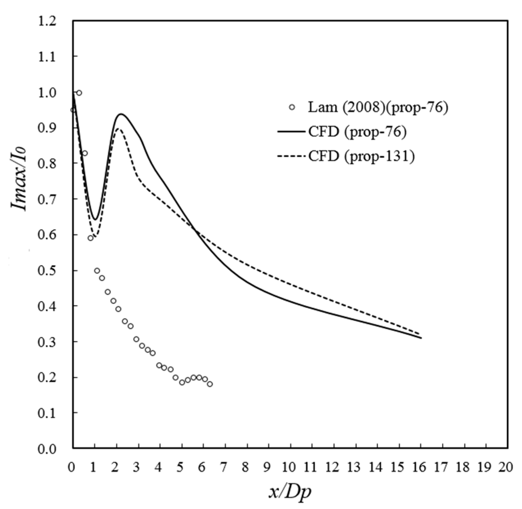
5.2. Turbulence Intensity Decay

Lam [15] measured the decay of the turbulent kinetic energy k of Propeller-76. The maximum turbulence intensity decay from Lam’s data [15] and the CFD results is compared in Figure 16. Lam’s experimental results [15] showed that the turbulence intensity of a single propeller decayed with the jet diffusion. However, it is observed from the CFD results that the maximum turbulence intensity decayed from the efflux plane until $\mathrm{x}=1D_p$, reaching a minimum value of 0.65$I_0$ before increasing rapidly, reaching a peak value of 0.95$I_0$ at $\mathrm{x}=2D_p$, and gradually decreasing again. According to the CFD results, the jets of the two propellers mixed exactly at approximately $\mathrm{x}=2D_p$. This may have led to an increase in the turbulence intensity from $\mathrm{x}=1D_p$ to $\mathrm{x}=2.5D_p$. The combination of the twin propeller jet made the turbulence superimposed on each other. The wake fluctuated more violently. Subsequently, as the jet continued to diffuse, the turbulence intensity decayed more slowly. Based on the CFD results, the turbulence intensity decay of the twin-propeller jet can be expressed as Equation (13).

$$\begin{array}{c}\frac{I_{max}}{I_0}=0.295{\left(\frac{\mathrm{x}}{D_p}\right)}^2-0.677\left(\frac{\mathrm{x}}{D_p}\right)+1\hspace{1em}\frac{\mathrm{x}}{D_p}<2\\ \frac{I_{max}}{I_0}=1.78{\left(\frac{\mathrm{x}}{D_p}\right)}^{-0.651}\hspace{1em}\frac{\mathrm{x}}{D_p}>2\end{array}$$

(13)

6. Conclusions

The current investigation demonstrates the flow structure of Twin-propeller-76 and Twin-propeller-131. The CFD results were verified by a model test of the ADV measurement. The velocity distribution and decay with turbulence intensities within the twin-propeller jets were compared with those in previous studies. The following contributions are presented.

(1)

The reliability of the CFD results was verified using an ADV measurement test. The dimensionless axial velocity distribution on the efflux plane measured experimentally and simulated by CFD showed four peaks. The diffusion of the experimental twin-propeller jet was more obvious than the diffusion in the CFD simulation and the dimensionless turbulence intensity measured by the ADV was greater.

(2)

The axial, tangential, and radial velocity distributions, and turbulence intensities of Propeller-76 and Propeller-131 were essentially the same. The prediction equation of efflux velocity ($V_0=1.59n{D}_p\sqrt{C_t}$) and its position ($R_{mo}=0.85\left(R_p-R_h\right)$) were suggested to predict the axial velocity on the efflux plane.

(3)

Twin-Propeller-76 and Twin-Propeller-131 exhibited similar decays for axial, tangential, and radial velocities. Several equations for predicting tangential and radial velocity decay were presented.

Type of Decay	Proposed Equation	Range
Axial velocity decay	$\frac{V_{max}}{V_0}=1$	$0\le x/D_p<0.35$
	$\frac{V_{max}}{V_0}=1.51-0.175\left(\frac{x}{D_p}\right)-0.46P^{\prime }$	$0.35\le x/D_p<3.5$
	$\frac{V_{max}}{V_0}=1.1{\left(x/D_p\right)}^{-0.58}$	$3.5\le x/D_p<14$; $14\le xDp$
Tangential velocity decay	$\frac{V_{tmax}}{V_{t0}}=-0.6492\left(\frac{x}{D_p}\right)+0.9749$	$0<x/D_p<0.79$
	$\frac{V_{tmax}}{V_{t0}}=0.7031e^{-0.4998\left(\frac{x}{D_p}\right)}$	$0.79\le x/D_p\le 6.32$
Radial velocity decay	$\frac{V_{rmax}}{V_{r0}}=e^{-0.283\frac{x}{D_p}}$	$0<x/D_p<2.4$
	$\frac{V_{rmax}}{V_{r0}}=-0.65\left(\frac{x}{D_p}\right)+2.06$	$2.4<x/D_p$
Turbulence intensity decay	$\frac{I_{max}}{I_0}=0.295{\left(\frac{\mathrm{x}}{D_p}\right)}^2-0.677\left(\frac{\mathrm{x}}{D_p}\right)+1$	$\frac{\mathrm{x}}{D_p}<2$
	$\frac{I_{max}}{I_0}=1.78{\left(\frac{\mathrm{x}}{D_p}\right)}^{-0.651}$	$\frac{\mathrm{x}}{D_p}>2$

(4)

For Twin-propeller-76, the length of ZFE-TP-4P was 3.5$D_p$, compared with 5.2$D_p$ for Twin-propeller-131. The length of the zone of flow establishment ($x_{0tp}$) was 14$D_p$ for Twin-propeller-76, compared with 14.5$D_p$ for Twin-propeller-131. The length of ZFE-TP-NI ($L_{ni}$. ) for Twin-propeller-76 was 2.3$D_p$, compared with 2$D_p$ for Twin-propeller-131. $x_{0tp}$ and $L_{ni}$ were not obviously affected by the propeller type.

References

1. Albertson, M.L.; Dai, Y.B.; Jensen, R.A.; Rouse, H. Diffusion of Submerged Jets. Am. Soc. Civ. Eng. 1950, 115, 639–697. [Google Scholar]
2. Hamill, G.A. Characteristics of the Screw Wash of a Manoeuvring Ship and the Resulting Bed Scour. Ph.D. Thesis, Queen’s University of Belfast, Belfast, UK, 1987. [Google Scholar]
3. Lam, W.H.; Hamill, G.A.; Robinson, D.J.; Raghunathan, S.; Song, Y.C. Analysis of the 3D zone of flow establishment from a ship’s propeller. KSCE J. Civ. Eng. 2012, 16, 465–477. [Google Scholar] [CrossRef]
4. Lam, W.H.; Hamill, G.A.; Robinson, D.J. Initial wash profiles from a ship propeller using CFD method. Ocean Eng. 2013, 72, 257–266. [Google Scholar] [CrossRef]
5. Guo, H.P.; Zou, Z.J.; Wang, F.; Liu, Y. Numerical investigation on the asymmetric propeller behavior of a twin-screw ship during maneuvers by using RANS method. Ocean Eng. 2020, 200. [Google Scholar] [CrossRef]
6. Huang, Y.S.; Yang, J.; Yang, C.J. Numerical prediction of the effective wake profiles of a high-speed underwater vehicle with contra-rotating propellers. Appl. Ocean Res. 2019, 84, 242–249. [Google Scholar] [CrossRef]
7. Prabhu, J.J.; Dash, A.K.; Nagarajan, V.; Sha, O.P. On the hydrodynamic loading of marine cycloidal propeller during maneuvering. Appl. Ocean Res. 2019, 86, 87–110. [Google Scholar] [CrossRef]
8. Ohashi, K. Numerical study of roughness model effect including low-Reynolds number model and wall function method at actual ship scale. J. Mar. Sci. Technol. 2020, 1–13. [Google Scholar] [CrossRef]
9. Zhang, H.; Li, D.; Luo, S.; Jia, M.; Sun, Z.; Li, Y.; Zhen, Z.; Zhang, X. Investigation of jet flow profiles from a navigating ship’s propeller. J. Appl. Sci. Eng. 2019, 22, 221–232. [Google Scholar] [CrossRef]
10. Abramowicz-Gerigk, T.; Gerigk, M.K. Experimental study on the selected aspects of bow thruster generated flow field at ship zero-speed conditions. Ocean Eng. 2020, 209. [Google Scholar] [CrossRef]
11. Wu, T.; Deng, R.; Luo, W.; Guo, C. 3D3C wake field measurement, reconstruction and spatial distribution study of ship using PIV. Huazhong Ligong Daxue Xuebao 2020, 48, 35–40. [Google Scholar] [CrossRef]
12. Jiang, J.; Lam, W.H.; Cui, Y.; Zhang, T.; Sun, C.; Guo, J.; Ma, Y.; Wang, S.; Hamill, G. Ship Twin-propeller Jet Model used to Predict the Initial Velocity and Velocity Distribution within Diffusing Jet. KSCE J. Civ. Eng. 2019, 23, 1118–1131. [Google Scholar] [CrossRef] [Green Version]
13. Mujal-Colilles, A.; Gironella, X.; Sanchez-Arcilla, A.; Puig Polo, C.; Garcia-Leon, M. Erosion caused by propeller jets in a low energy harbour basin. J. Hydraul. Res. 2017, 55, 121–128. [Google Scholar] [CrossRef] [Green Version]
14. ANSYS Fluent. ANSYS Fluent User’s Guide 15.0; ANSYS Inc.: Canonsburg, PA, USA, 2013. [Google Scholar]
15. Lam, W.H. Simulations of a Ship’s Propeller Jet. Ph.D. Thesis, Queen’s University of Belfast, Belfast, UK, 2008. [Google Scholar]
16. Versteeg, H.K.; Malalasekera, W. An Introduction to Computational Fluid Dynamics the Finite Volume Method, 2nd ed.; Prentice Hall: Essex, UK, 2007. [Google Scholar]
17. Cui, Y.; Lam, W.H.; Zhang, T.; Sun, C.; Robinson, D.; Hamill, G. Temporal model for ship twin-propeller jet induced sandbed scour. J. Mar. Sci. Eng. 2019, 7, 339. [Google Scholar] [CrossRef] [Green Version]
18. Stewart, D.P.J. Characteristics of a Ship’s Screw Wash and the Influence of Quay Wall Proximity. Ph.D. Thesis, Queen’s University of Belfast, Belfast, UK, 1992. [Google Scholar]
19. Berger, W.; Felkel, K.; Hager, M.; Oebius, H.; Schale, E. Courant provoque parles bateaux protection des berges et solution pour eviter l’erosion du lit duhaut rhin. In Proceedings of the 25th Congress P.I.A.N.C., Edinburgh, Scotland, 10–16 May 1981. Section 1-1. [Google Scholar]
20. McGarvey, J.A. The Influence of the Rudder on the Hydrodynamics and the Resulting Bed Scour of a Ship’s Screw Wash. Ph.D. Thesis, Queen’s University of Belfast, Belfast, UK, 1996. [Google Scholar]
21. Prosser, M.J. Propeller induced scour. In BHRA Project RP A01415; The Fluid Engineering Centre: Cranfield, UK, 1986. [Google Scholar]
22. Hamill, G.A.; Kee, C.; Ryan, D. 3D Efflux Velocity Characteristics of Marine Propeller Jets. Proc. Inst. Civ. Eng. Marit. Eng. 2015, 168, 62–75. [Google Scholar]
23. Mujal-Colilles, A.; Gironella, X.; Crespo, A.J.C.; Sanchez-Arcilla, A. Study of the bed velocity induced by twin propellers. J. Waterw. Port Coast. Ocean Eng. 2017, 143, 04017013. [Google Scholar] [CrossRef] [Green Version]
24. Fuehrer, M.; Römisch, K. Effects of modern ship traffic on islands and ocean waterways and their structures. In Proceedings of the 24th Congress P.I.A.N.C., Leningrad, Russia, September 1977. Section 1-3. [Google Scholar]
Figure 1. Geometric model of propellers: (a) Propeller-76; (b) Propeller-131.
Jmse 08 01025 g001
Figure 2. Meshed twin-propeller system: (a) Water subdomain of Twin-propeller-76; (b) Water subdomain of Twin-propeller-131. Arrow shows the zoom-in on a particular part.
Jmse 08 01025 g002
Figure 3. Experiment setup: (a) Front view; (b) Axial view.
Jmse 08 01025 g003aJmse 08 01025 g003b
Figure 4. Axial velocity distribution at 1Dp within ZFE-TP-4P.
Jmse 08 01025 g004
Figure 5. Turbulence intensity distribution at 11Dp within ZFE-TP-4P.
Jmse 08 01025 g005
Figure 6. Diagram of efflux velocity derivation, where are zone (A) the far upstream, zone (B) the immediate upstream, zone (C) the immediate downstream, and zone (D) the far downstream [15].
Jmse 08 01025 g006
Figure 7. Axial velocity distributions at the efflux plane.
Jmse 08 01025 g007
Figure 8. Axial velocity decay.
Jmse 08 01025 g008
Figure 9. Axial velocity decay within different zones: (a) ZFE-TP-4P; (b) ZFE-TP-2P; (c) Zone of established flow.
Jmse 08 01025 g009
Figure 10. Axial velocity distributions within different zones: (a) 1.6Dp within ZFE-TP-4P; (b) 8Dp within ZFE-TP-2P; (c) 18Dp within zone of established flow.
Jmse 08 01025 g010
Figure 11. Tangential velocity distributions at the efflux plane.
Jmse 08 01025 g011
Figure 12. Tangential velocity decay.
Jmse 08 01025 g012
Figure 13. Radial velocity distributions at the efflux plane.
Jmse 08 01025 g013
Figure 14. Radial velocity decay.
Jmse 08 01025 g014
Figure 15. Turbulence intensity distributions at efflux plane.
Jmse 08 01025 g015
Figure 16. Turbulence intensity decay.
Jmse 08 01025 g016