Experimental Observation on Beach Evolution Process with Presence of Artificial Submerged Sand Bar and Reef

Abstract

For observation on the influence mechanism of environmentally and aesthetically friendly artificial submerged sand bars and reefs in a process-based way, a set of experiments was conducted in a 50 m-long flume to reproduce the cross-shore beach morphodynamic process under four irregular wave conditions. The beach behavior is characterized by the scarp (indicating erosion) and the breaker bar (indicating deposition), respectively, and the scarp location can be formulated as a linear equation regarding the natural exponential of the duration time. Overall, main conclusions are: (1) the cross-shore structure of significant wave height and set-up is mainly determined by the artificial reef (AR); (2) the cross-shore distribution of wave skewness, asymmetry, and undertow (indicating shoaling and breaking) is more affected by the artificial submerged sand bar (ASB); (3) the ASB deforms and loses its sand as it attenuates incident waves, which leads to a complex sediment transport pattern; (4) the scarp retreat is related to the beach state, which can be changed by the AR and the ASB; (5) the AR, the ASB, and their combination decrease wave attack on the beach. In conclusion, this study proves positive effects of the AR and the ASB in beach protection through their process-based influences on beach behaviors and beach states for erosive waves.

1. Introduction

Coastal erosion is a problem at many coastal sites, caused by natural effects as well as human activities [1,2], and the remedial measures fall into soft and hard engineering. Soft engineering is the mechanical placement of material on the beach (beach nourishment) or within the nearshore area (shoreface or bar nourishment). Beach nourishment, introduced in the 1920s [3], is now a technique used world-wide to maintain the eroding beaches along sandy coasts [4,5,6,7]. The U.S. Atlantic coast has confirmed the positive feedback between coastal development and beach nourishment for decades [8], where the mean rate of shoreline change has reversed from −55 cm/year (erosion) prior to 1960 to about +5 cm/year (accretion) after 1960, despite inevitable shoreline retreat over large spatial scales around the world due to the rising sea-level [9]. Shoreface nourishment, introduced in the 1990s, acts as a wave filter such as reef and meanwhile aims at nourishing the nearshore zone with long-term processes [10,11,12]. However, the performance of shoreface nourishment is less effective than beach nourishment [5], because the nourished sand is redistributed by both cross-shore and long-shore transport. Generally, the effect and the longevity of soft nourishment vary greatly from place to place due to multiple factors in the complex coastal process. Beyond those, the long-term ecological influence [13,14,15,16] and the material borrowed site [17,18,19,20] are the current challenges at different levels for various coasts. Hence, soft nourishment is not economically or environmentally suitable for some sites and can even lead to an erosion “hot spot” in a successful nourishment [21], and proper structures are still needed for erosion control.

Meanwhile, hard engineering structures were designed to perform multiple functions among the natural coastal processes and basically comprise groynes, detached breakwaters, and reefs [1]. Detailed and complete investigations on the efficiency and the impact of natural and artificial structures in recent decades were carried out from the perspective of shoreline management [22,23,24], with important experiences and conclusions. First, positive attitudes were expressed towards natural reefs and stream deltas [22]. As an alternative method for dealing with increasing erosion pressures with limited resources, artificial reefs range from rock mounds parallel to the shore to prefabricated units with various types of structures, such as a concrete box, tunnel, dome, leg, or more complex shapes [25,26] with features of submergence and porosity. The deployment objectives in recent research have shifted from improving fisheries as a resource to rehabilitation of the marine ecosystem, improving surfing or diving conditions, recreational fishing, and coastline protection [27]. Second, some structures are most effective when coupled with other measures. For example, low crest structures (LCSs) perform well when groynes acting as artificial headlands are present and can help retain the nourished sand. Since many coasts have already built engineering structures, further design should incorporate and utilize the effect of the existing coastal structures [28,29,30,31]. In addition, modified structures such as submerged artificial headlands (SAH) and detached artificial headlands (DAH) were applied to enhance the water exchange and thus improve the water environment [32]. Third, the key problems, pointed out by Ranasinghe and Turner [33] and associated with but not limited to the use of LCSs, are the identification of environmental and structural parameters governing the mode (i.e., erosion or accretion), the magnitude (e.g., size of salient), and the response of the adjacent shoreline. The morphodynamic mode refers to the fundamental principle and the hydrodynamic and sediment mechanism, which is yet to be fully understood, and the latter emphasizes the longshore current and sediment transport.

Field measurements detailed the phenomena of hydrodynamic and morphological evolution of the nearshore area [34] with structures [35,36], beach nourishment [37,38,39,40], and shoreface nourishment [41,42,43,44,45,46], which also provided the foundation for the establishment of prediction models using numerical simulation [47,48,49,50,51,52]. Basin experimental models were scaled down from the prototype to test the influence of engineering scenarios on both cross-shore and long-shore processes [53,54,55,56]. For the cross-shore responses to extreme surge or wave conditions, large-scale flume experiment projects [57,58,59,60,61] were carried out to elucidate the cross-shore (shoaling, surf, and swash zone) physical processes of the morphodynamic system. Furthermore, the cross-shore hydrodynamic forces and the resulting sediment transport mechanism have been continuously investigated by fixed-bed and movable-bed flume experiments for typical profiles of dune beaches, beaches with bars and reef flat, and barriers. Achievements were made in short wave and infragravity wave dynamics, wave skewness, undertow, boundary-layer dynamics, and the relation with sediment transport [62,63,64,65,66,67] under a range of wave conditions (regular, bichromatic, and random waves). For typical fine beach sand (e.g., 0.1–0.5 mm), using natural sand scaling by geometric ratio in small wave flume may lead to model sand moving as silt, not sand. Hence, a series of light-weight model (LWM) experiments [68,69,70,71,72] were designed using light-weight model sand to cover the modeling of a fine sand beach profile, especially a large cross-shore area in a limited flume length. In spite of all the extensive research, it is still difficult to make a direct estimation of the nearshore influence of multiple measures. For instance, even for an offshore structure or a sand berm, hydrodynamic and morphodynamic changes are delicate for its cross-shore location, not to mention the increasingly complex coastal situation with integrated engineering. Besides, some questions remain to be answered: is there any difference between the actions of soft and hard interventions on the erosion features?; how do they differ from each other in a morphodynamic system?; when a combination of measures is used, which of them can be taken as having the primary impact on the hydrodynamic and sediment processes in shoaling, surfing, and swash zones?

To answer these questions, further research is needed to investigate the influence regime of soft and hard interventions on the morphodynamic mechanism. From these perspectives, we designed a set of movable bed experiments on the basis of the Beidaihe nourishment programs to investigate the cross-shore morphodynamics in this study. Beidaihe in Hebei Province, China is a famous national tourist destination and a demonstration site of beach nourishment, where submerged breakwaters (in the form of prefabricated sandbags and artificial reefs), artificial headlands (made of rippled-rock), submerged sand bars, grouted rubble revetments, and groynes were built. These offshore interventions are important elements in the whole beach restoration design. Their proper adoption may help to reduce the erosion by large waves without further sand filling and yet barely affect the water environment and aesthetic aspects.

The novelties of this process-based study include: (1) two ecological offshore interventions, i.e., artificial submerged sand bar (ASB) and artificial reef (AR), were firstly experimentally investigated for their combination influences on cross-shore hydrodynamic and morphological process; (2) the comparison was made of morphodynamic responses to individual ASB, AR, and the combination of them; (3) quantitative relations of scarp and breaker bar (indicating beach erosion and deposition process, respectively) were established, which illustrated the influence mechanism of the offshore interventions; (4) the changed wave breaking and morphological features were found to be linked with overall morphodynamic state, which implied the role of offshore interventions in beach system.

2. Method

For the prototype area Beidaihe of the experiment, the tides are regular diurnal with a multi-annual average tidal range of 0.74 m. Most of the time, beaches are exposed to a low-energy wave climate, i.e., about 91.23% of the recorded significant wave heights (Hs) are less than 0.6 m and only 1.01% of Hs over 0.9 m, and the average peak period (Tp) is 4.5 s. However, the relatively stable beach profiles still suffered summer storm waves attack with wave height over 2.0 m, and some “hot spots” (severe erosion locations) were found. The movable bed experiment (Figure 1) was conducted in a wave flume (50 m long, 0.8 m wide, and 1.2 m deep) at the Laboratory of Hydraulic and Harbour Engineering, Tongji University to simulate the cross-shore morphological evolution of fine-sand beach profiles under complex hydrodynamic processes in surf and swash zones. As a grain size range of 0.1–0.5 mm was involved, a light-weight model was adopted to reduce the scale effects due to limitations of the experimental facilities. Only half of the flume width was used, causing the width of bed model to be 0.40 m, which enabled the long-shore uniformity of morphological changes. Four model wave conditions (J1–J4) were generated by a piston-type wave generator with active reflection compensation based on the field measurements, as detailed in

Table 1. Physical experimental tests (N represents mild profile part without the offshore interventions, and beach with artificial reef (B-AR), beach with artificial submerged sand bar (B-ASB), and B-ASB-AR indicate beach with artificial reef and artificial submerged sand bar).

Test Name	Wave		Profile Type	Test Name	Wave		Profile Type
	Hs (m)	Tp (s)			Hs (m)	Tp (s)
B-N-J1	0.04	1.20	Beach (B-N)	B-ASB-J1	0.04	1.20	Beach with ASB (B-ASB)
B-N-J2	0.07	1.44		B-ASB-J2	0.07	1.44
B-N-J3	0.10	1.57		B-ASB-J3	0.10	1.57
B-N-J4	0.13	1.77		B-ASB-J4	0.13	1.77
B-AR-J1	0.04	1.20	Beach with AR (B-AR)	B-ASB-AR-J1	0.04	1.20	Beach with ASB and AR (B-ASB-AR)
B-AR-J2	0.07	1.44		B-ASB-AR-J2	0.07	1.44
B-AR-J3	0.10	1.57		B-ASB-AR-J3	0.10	1.57
B-AR-J4	0.13	1.77		B-ASB-AR-J4	0.13	1.77

.

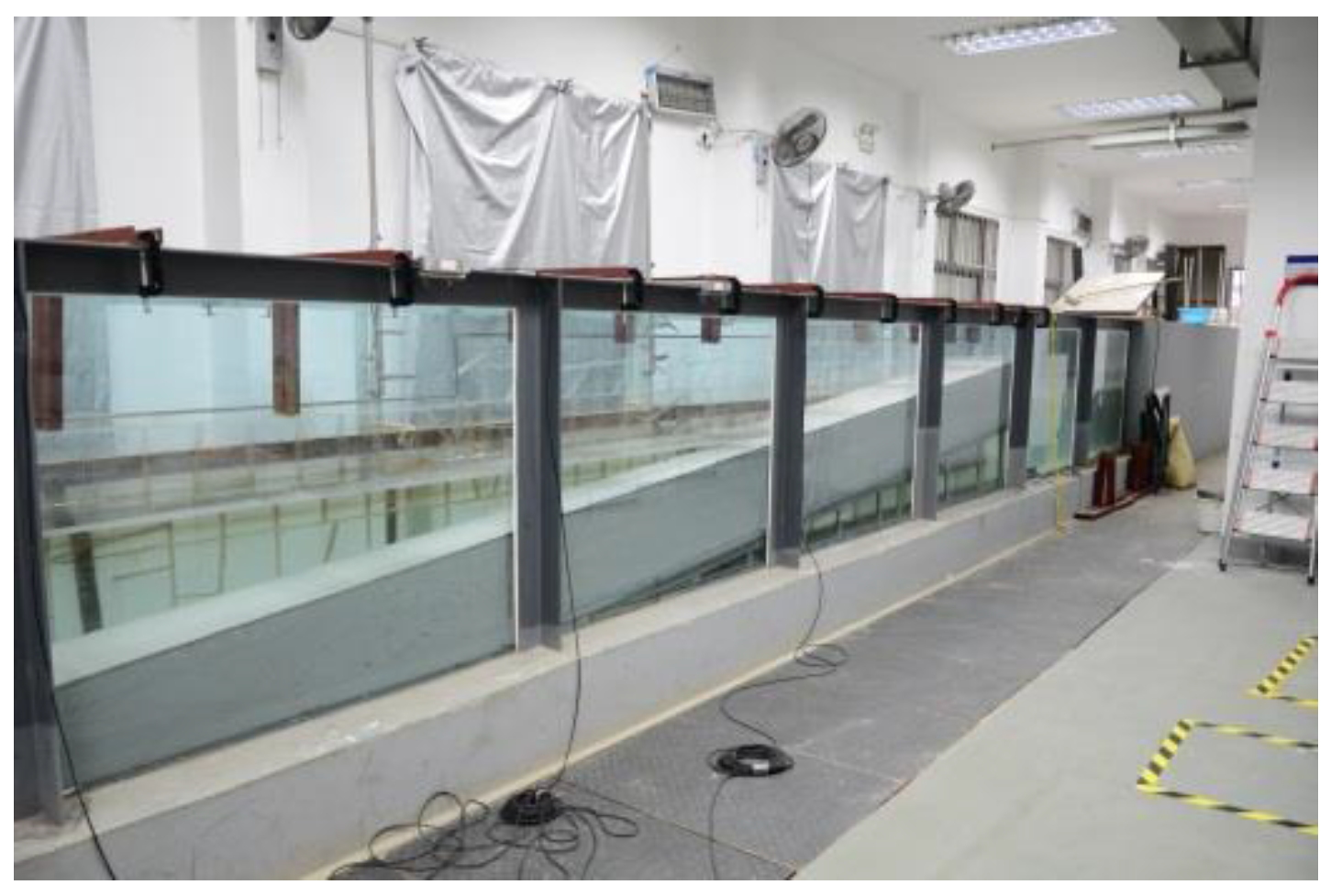
2.1. Experimental Design and Instrumentation

The adoption of light-weight sediment particles with a lower density yet coarser grain size than natural sand [73] means that the sediment grain size is not scaled by the geometric scale yet leads to basically the same incipient motion and settling process. The relaxation on the similitude of the geometric particles indicated the focus on the similarity of the evolution rate, rather than its duration, to the final morphology [74].

In this study, the beach profile model was made of resin sand to reproduce the evolution feature. The density of the resin sand was 1.40–1.45 g/cm³ with grain size ranging from 0.15 to 0.18 mm, which maintained the similitude of the hydrodynamic and sediment process by satisfying the Froude number, the Shields number, and the Rouse number under the geometric scale factor of 10 (prototype/model). The details of the scaling calculations can be found in [75].

Considering the capacity and the precision of the wave maker under the condition of model scaling, four sets of characteristic wave height and period were selected, which covered normal, moderate, and storm conditions. Four irregular model waves were generated based on these parameters shown in Table 1, and the control point was located at the front side of AR with water depth of 0.47 m. The maximum values of measured profile slopes in the field were adopted, i.e., the beach slope just after the nourishment was 1:10, and the average offshore slope was 1:200. As shown in Figure 2, four cross-shore beach profile types were investigated: (a) a nourished beach with a slope of 1:10 and a mild shore-face part with a slope of 1:200 (profile type named as B-N); (b) a beach with an AR installed 20 m offshore the beach (profile type named as B-AR); (c) a beach with an ASB placed 10 m offshore (profile type named as B-ASB); and (d) a beach with both an AR and an ASB located as in B-AR and B-ASB (profile type named as B-ASB-AR). The movable bed was obstructed by a fixed end offshore with slope of 1:10. A total of 16 experimental tests were conducted with the same duration of 90 min, as listed in Table 1. The model AR was 1.80 m long and 0.30 m high and consisted of polymethyl methacrylate blocks. The ASB was an isosceles trapezoid shape with the crest width of 3.00 m and depth of 0.20 m and slopes of 1:10. The coordinate system for comparison analysis is shown in Figure 2a.

Hydrodynamic measurements were made by 13 pre-calibrated capacitive-type wave gauges (with accuracy of ±2 mm) and three acoustic doppler velocimeters (ADVLab, Nortek, with an accuracy of 0.5% of measurement ±1 mm/s) in a fixed cross-shore arrangement as in

Table 2. The horizontal positions of instruments (unit: m).

	Profile Type	B-N	B-AR	B-ASB	B-ASB-AR
Wave Gauges
W1		23.30	23.30	23.30	23.30
W2		22.65	22.65	22.03	22.03
W3		20.78	20.78	20.78	20.78
W4		19.80	19.80	19.80	19.80
W5		18.12	18.12	18.12	18.12
W6		16.25	16.25	16.25	16.25
W7		14.50	14.50	14.50	14.50
W8		13.12	13.12	13.12	13.12
W9		11.47	11.47	11.47	11.47
W10		9.67	9.67	9.67	9.67
W11		8.00	8.00	8.00	8.00
W12		5.21	5.21	5.21	5.21
W13		2.01	2.01	2.01	2.01
V1		22.03	22.03	15.72	15.72
V2		21.44	21.44	12.51	12.51
V3		20.33	20.33	10.23	10.23

. Among all the tests, the most significant profile change was found in the beach and ASB area during the evolution process captured by videos. The final profiles were obtained from photos, which were calibrated by rulers fixed on the side-wall of the flume. The geometric accuracy was estimated to be 3 mm for video images and 2 mm for photos.

2.2. Data Analysis

The water levels and velocity components directly measured by wave gauge and ADV provided the transformation of wave energy and wave shape. Then, the characteristics of the bed profiles were achieved with a local dynamic changing process. The undertow and the total sediment transport were estimated from wave and topography measurements.

2.2.1. Hydrodynamics

The mean water level at each wave gauge indicated the wave set-up and set-down for positive and negative values. Spectral analysis (using Welch’s approach) was conducted to calculate the significant wave height using 10 min-long data excluding a start period of 60 s.

Waves contribute to onshore sediment transport by the non-linear wave shape of the incident waves and induce streaming in the wave boundary layer, while offshore transport is related to return flow and phase coupling between wave groups and accompanying (bound) long waves [76]. In nearshore areas where the intra-wave kinematics are crucial, these mechanisms are described by parameterization, as the detailed processes are difficult to isolate from each other. In this study, these parameters were compared for different profile types to determine the influences induced by the AR or the ASB.

In addition to the significant wave height Hs, a representative long wave height H_{s_long} for wave energy in the low-frequency band (0.004–0.05 Hz, 20–250 s) [77] was calculated using the same method as for H_s with the frequency domain scaled down to the model scale, corresponding to 0.01–0.15 Hz (6.67–100 s).

The wave skewness and asymmetry were estimated by Equation (1) and Equation (2) based on the water level fluctuations [78,79,80].

$$Sk=\frac{\langle {\left(\eta -\overline{\eta }\right)}^3\rangle }{\langle {\left(\eta -\overline{\eta }\right)}^2\rangle {}^{3/2}},$$

(1)

$$Asy=\frac{\langle {\mathscr{H}}^3\left(\eta -\overline{\eta }\right)\rangle }{\langle {\left(\eta -\overline{\eta }\right)}^2\rangle {}^{3/2}},$$

(2)

where $\eta$ is the free surface elevation, $\overline{\eta }$ is the wave set-up, and $\langle -\rangle$ is the time averaging operator; $\mathscr{H}$ is the Hilbert transform. A larger value of Sk indicates larger bed shear stresses at the wave crest than at the wave trough, which indicates the tendency of the wave crest to carry the suspended sediment onshore. Abrupt accelerations (Asy) are associated with thinner boundary layers and thus higher bed shear stresses for a given velocity magnitude [81].

The undertow $\overline{u}$ (offshore-directed depth-averaged current forced by the wave energy dissipation) was estimated as the balance due to a shoreward mass flux including wave-induced (Q_w) and roller-induced (Q_r) mass flux [80]:

$$\overline{u}\left(h_0+\overline{\eta }\right)=-Q_w-Q_r,$$

(3)

$$Q_w=\frac{c}{h_0}\overline{{\eta }^2}-\frac{c}{h_0^2}\overline{{\eta }^3},$$

(4)

$$Q_r=\frac{{\rho }_r{A}_r}{\rho T_p},$$

(5)

where h₀ is the water depth at rest, c is the wave speed, ${\rho }_r$ is the density of the fluid in the aerated roller taken as a constant 650 kg/m³, A_r is the roller area, and T_p is the peak period. Equation (4) is used to estimate Q_w based on the assumption that the orbital velocity does not vary vertically. The roller area is given by A_r = 0.9H², where H is the local wave height [82]. The growth of $\overline{u}$ is hereinafter referred to as the growth in its absolute value.

The raw data of velocity components should be pre-processed before any calculation because of the measurement principles. The velocity data should be excluded when the correlation (COR) of the ADV data is less than 70% or the SNR (Signal Noise Ratio) is less than 20 dB. Then, the spikes were detected using the 3D phase-space thresholding method [83] and were replaced by cubic interpolation in this study. Based on the modified velocity series, the Shields number $\theta$ was calculated as follows:

$$\theta =\frac{0.5\rho f_w{U}_w^2}{\left({\rho }_s-\rho \right)gD},$$

(6)

where ${\rho }_s$ is the density of the sediment particle, and $\rho$ is the water density, g is the gravitational acceleration, D is the sediment grain size, U_w is the bottom orbital velocity of wave, and f_w is the wave friction coefficient calculated by the method of Soulsby [84], covering the identification of a laminar, smooth turbulent or rough turbulent regime.

$$f_w=B{\left(R_w\right)}^{-N} \mathrm{for} \mathrm{laminar} \mathrm{and} \mathrm{smooth} \mathrm{turbulent} \mathrm{regime},$$

(7)

$$f_w=0.237{\left(\frac{A}{k_s}\right)}^{-0.52} \mathrm{for} \mathrm{rough} \mathrm{turbulent} \mathrm{regime},$$

(8)

where $R_w=\frac{U_{w}A}{\nu }$ is the wave Reynolds number; B = 2, N = 0.16 for the laminar flow and B = 0.0521, N = 0.187 for the smooth turbulent flow; $A=U_{w}T/2\pi$ is the semi-orbital excursion of wave orbital motion at the edge of the boundary layer, and T_p is used for T here. k_s is the Nikuradse equivalent sand grain roughness, being 2.5D₅₀. The Shields numbers at wave gauges calculated by Soulsby method can be verified by the results calculated from ADV measurement.

2.2.2. Profile Morphology

As the incident waves propagated onshore, the beach face was eroded, showing the vertical cut, usually called the wave-attack scarp. Meanwhile, the eroded sand was transported offshore and formed an underwater bar named a breaker bar. Therefore, the beach profile analysis focused on the development of the scarp and the breaker bar to investigate the influences of different nourishment strategies.

The top and the bottom positions of beach scarp were calculated from minimum and maximum values of the second derivative of the measured profiles [85]. In this study, the larger horizontal coordinate (sx) of the two limits was chosen as the final scarp location for analysis. The height of the breaker bar was defined as the maximum deposition thickness z_bar (the maximum elevation relative to the initial bed level) with its location at the horizontal coordinate of x_bar. All above location indicators are shown in Figure 3.

In addition, some sand ripple appeared on the fore-slope and the crest of the ASB, with a maximum length and height of 5.80 cm and 0.60 cm, respectively, which barely affected the large-scale morphological changes on the beach.

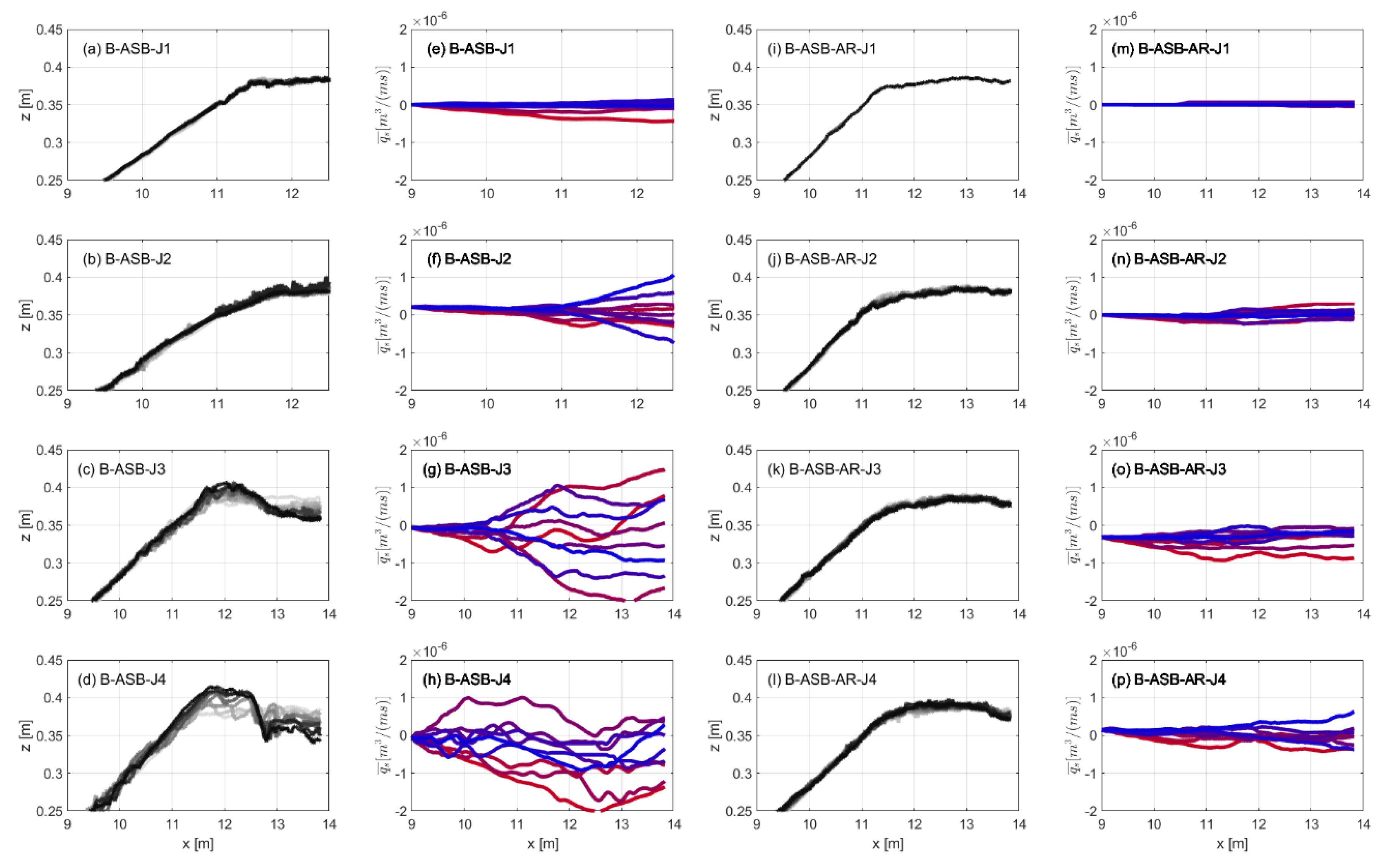
2.2.3. Sediment Transport

The total sediment transport rate $\overline{q_s}$ was estimated using the sediment mass conservation equation based on the difference between captured beach profiles as in Equation (9):

$$\frac{\partial q_s}{\partial \mathrm{x}}=-\left(1-p\right)\frac{\partial z}{\partial t},$$

(9)

where q_s is the instantaneous sediment transport rate, z is the bottom elevation at the cross-shore position x, and p is the sediment bed porosity, assumed to be loosely packed and homogeneous along the beach profile (p = 0.4 used here). The total transport rate at x = 0 is set to be zero. Therefore, the $\overline{q_s}$ at a given cross-shore location x during a wave climate duration $\mathsf{\Delta }t$ can be obtained by the discrete version of Equation (10) with the measured bed level changes ($\mathsf{\Delta }{z}_b$):

$$\overline{q_s}\left(x\right)=\overline{q_s}\left(x-\mathsf{\Delta }x\right)-\mathsf{\Delta }x\left(1-p\right)\frac{\mathsf{\Delta }{z}_b}{\mathsf{\Delta }t},$$

(10)

where $\overline{q_s}>0$ ($\overline{q_s}<0$) corresponds to the onshore (offshore) sediment transport.

3. Results

In this section, the experimental results are presented in terms of different profile types. First, the hydrodynamic patterns along the profiles were analyzed by parameterization of the wave processes. Then, the profile evolution comprising the scarp and the breaker bar was unified by model establishment to enable comparison among the four profile types. Finally, the effect of the ASB was studied on the deformation process, with analysis of the influence of the AR offshore.

3.1. Hydrodynamics

The cross-shore changes of hydrodynamic and sediment transport are illustrated in Figure 4. The complex coastal processes were analyzed by parameterization in terms of wave energy (significant wave height H_s, long wave height H_{s_long}), mean water level ($\overline{\eta }$), mass flux (wave skewness Sk, wave asymmetry Asy, and undertow $\overline{u}$) and the total sediment transport rate $\overline{q_s}$.

As Figure 4a1 shows, H_s in B-N decreased as the incident waves propagated onshore, despite slight local increases at W2, W7, and W9. The wave energy of the low frequency domain (Figure 4b1) decreased along the propagation, and a large incident wave generated large H_s-long at each wave gauge. The mean water level $\overline{\eta }$ (Figure 4c1) peaked at W11 for all incident waves, while there was another significant growth at W3‒W5 in B-N-J4. Hence, in addition to the main shoaling zone on the beach slope, there were two local areas with a relatively strong shoaling effect for J4 waves and one for J1‒J3. This was also verified by Sk (Figure 4d1), with peaks at the maximum dissipation. The negative Asy (Figure 4e1) with a large absolute value occurred at W2 and W1, representing intensive breaking. Correspondingly, the absolute value of undertow $\overline{u}$ (Figure 4f1) increased with the incident waves. The results of B-N were set as the basis to analyze the relative changes of results in the other profile types as follows.

In tests of B-AR, although the wave energy at W13 was slightly enhanced because of reflection by AR, H_s (Figure 4a2) and H_s-long (Figure 4b2) on its leeside were decreased, with maximum reductions of 0.05 m (at W5–W11) and 0.02 m (at W1 and W2), respectively. The reduction in wave energy was heightened with the incident wave energy. The shoaling effect was also reduced compared with B-N, and the peak of $\overline{\eta }$ at W11 was preserved only in B-AR-J4 (Figure 4c2). The Sk values at W1 and W2 were reduced under all wave climates (Figure 4d2). In the shoreface part, the Sk value increased at W4‒W9 and decreased at W10‒W13 in B-AR-J1. Then, as the incident wave grew, the wave gauge points turned to have decreased values relative to the corresponding B-N tests. For the cross-shore pattern of Asy (Figure 4e2), reduction in the absolute value at W1 meant weaker wave breaking relative to B-N. In the leeside of AR, $\overline{u}$ was decreased greatly in the range of 0.003–0.025 m/s, and $\overline{u}$ at W13 was increased by 0–0.009 m/s.

The influence of the ASB was more complex. In B-ASB-J1 and B-ASB-J2, H_s (Figure 4a3) and H_s-long (Figure 4b3) changed slightly, with the changes less than 0.003 m and 0.006 m, respectively, which showed a small growth in the crest and the fore-slope of the ASB. For the waves of J3 and J4, H_s barely changed at W11 and W13 but increased at W9‒W10 (by less than 0.006 m and 0.004 m for J3 and J4, respectively), covering the fore-slope and the fore-part of the crest, and then decreased significantly at W2‒W8 (by 13% and 23% for J3 and J4). Meanwhile, the cross-shore pattern of H_s-long was similar to that in the B-N test but was different on the beach. In particular, H_s and H_s-long at W1 were increased for J2 and J3, with the maximum growth of 0.011 m in H_s-long in B-ASB-J3. On the basis of $\overline{\eta }$, Sk and Asy (Figure 4c3,d3,e3), wave shoaling, breaking, and bottom friction due to the ASB predominated in the wave transformation of J2‒J4. Hence, there were local peaks of Sk and Asy between W6 and W10 covering the ASB, which indicated a stronger energy dissipation area rather than a beach slope. Moreover, $\overline{u}$ was reduced at W11‒W13 and increased around the ASB (Figure 4f3). Beyond that, the ASB decreased $\overline{u}$ in the lee-side in a wider range for larger incident waves.

In comparison with the results in B-AR and B-ASB, the cross-shore hydrodynamics in B-ASB-AR showed a mixture of both features. The wave energy attenuation in B-ASB-AR was similar to that in B-AR, and the maximum reduction of H_s (Figure 4a4) and H_s-long (Figure 4b4) ranged between 39% and 50%. The hydrodynamics at W11‒W13 depended on the AR rather than the ASB. Although $\overline{\eta }$ (Figure 4c4) resembled that in B-AR, Sk, Asy and $\overline{u}$ (Figure 4d4,e4,f4) changed in the same trend as those in B-ASB but with smaller absolute values. This was because the incident waves were attenuated by the AR before passing to the ASB, and bottom friction and wave breaking on the ASB further dissipated the wave energy before attack on the beach slope.

Generally, the cross-shore sediment transport coupled with wave breaking varied for different profile types. In B-N and B-AR, sediment transport was confined on the beach, where the upper beach was eroded, and sediment transported offshore until settlement at the lower area. Comparing Figure 4g1,g2, the maximum $\overline{q_s}$ was diminished by the AR (by 44‒64%), with the location moving shoreward under larger wave climates. In B-ASB and B-ASB-AR, the profile change could cover nearly the whole horizontal length, because the ASB itself covered about one-third of the whole profile and acted as a sediment source. The offshore sediment transport was generated on the beach and the fore-slope of the ASB, and onshore sediment barely existed in B-N and B-AR tests. Special cases were B-ASB-J4 and B-ASB-AR-J3, where onshore sediment transport dominated the area between the beach and the ASB.

3.2. Beach Profile Behavior

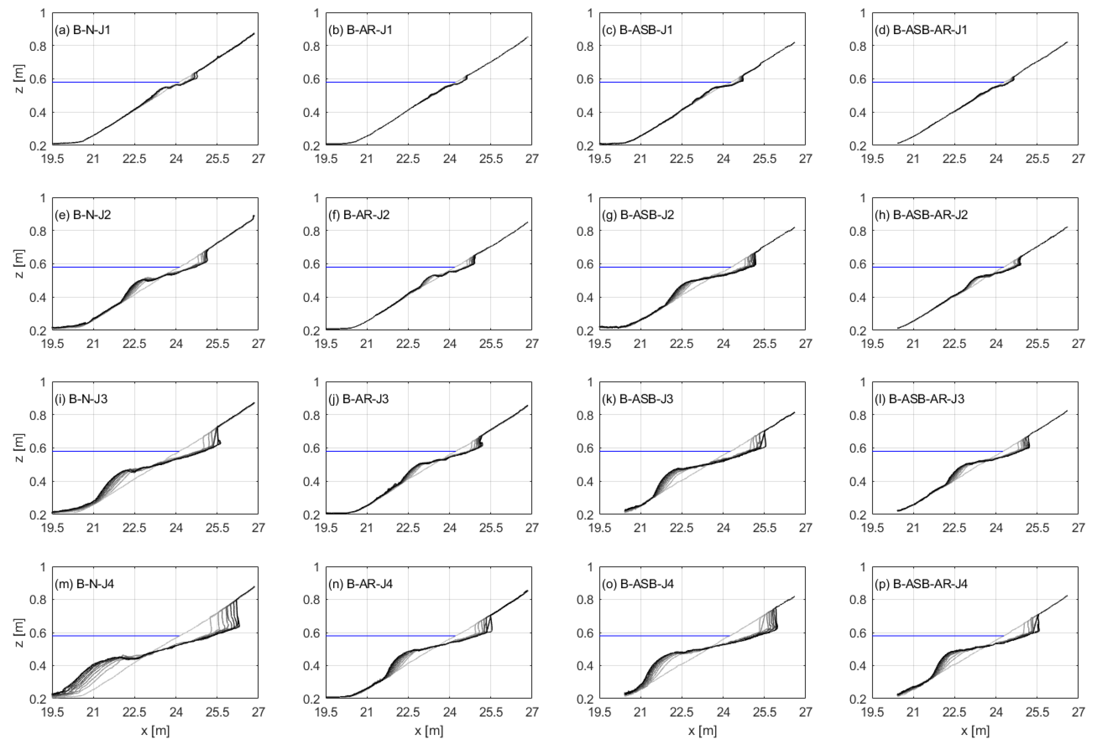
3.2.1. Evolution process

Beach nourishment often causes disturbances, e.g., beach scarps and dunes, that eventually equilibrate via sediment transport processes [85]. The beach face evolution (shown in Figure 5) in all the tests started with a typical post-nourishment scarp erosion process summarized by Erikson et al. [86] as follows: continued wave attack on the scarp (in the present study) or dune caused undercutting or notching (removal of scarp or dune foot), which led to the visible tension cracks in the upper part; the resulting overhang eventually turned into sand sliding downward or toppling over, leaving a vertical face. Then, the fallen sand was carried offshore by the undertow accompanied by further beach undercutting in the next cycle. As a result, the eroded sand settled and quickly formed a breaker bar, where wave breaking happened continuously. The breaker bar gradually increased in volume and migrated offshore and thus weakened the onshore wave attack, which impeded the recession of the scarp location. Overall, the AR, the ASB, and their combination significantly reduced the beach change (upper erosion and lower deposition) and also caused different morphodynamic features.

This study focused on the different influences induced by the AR and the ASB, individually and in combination, on the evolution process. Relations were found between the dimension indicators and the duration time. The fitting parameters were assumed to reflect the comprehensive impact of the incident waves and the nourishment method, which are explored in the Discussion section.

3.2.2. Scarp

The scarp erosion is related to wave run-up, which reflects the different influences due to the incident waves and the beach profiles. Based on the beach evolution process (Figure 5), the change of scarp location with time was derived with a time interval of 10 min, as in Figure 6, which shows that the scarp location gradually retreated with time at a decreasing rate. The retreat rate V_sx in each time interval was estimated by calculating the first derivative of the scarp location data sx over time t (V_sx = d(sx)/dt). It can be inferred that sx increased with t until V_sx monotonically reduced to zero, corresponding to the equilibrium state with the maximum sx. As a result, a natural exponential function (exp) was applied to capture this process feature, leading to a scarp retreat model consisting of Equations (11) and (12):

$$V_{sx}=V_0\times exp\left(-\frac{t}{T_e}\right),$$

(11)

$$sx=P2-P1\times exp\left(-\frac{t}{T_e}\right),$$

(12)

where the unit of t is minute. Equation (11) was firstly fitted to acquire parameter T_e, which was then used to fit the sx data on Equation (12) to obtain parameters P1 and P2.

The fitting results are illustrated in

Table 3. Fitting parameters with evaluations of the exponential model on scarp evolution. (SSE: The sum of squares due to error; RMSE: Root mean squared error; Adjusted R-square: Degree-of-freedom adjusted coefficient of determination).

	Parameters	Equation (11)			Equation (12)
Test		V0 (m/s)	Te (s)	Adj R-Square	P1 (m)	P2 (m)	SSE	RMSE	Adj R-Square
B-N-J1		0.0052	70.35	0.71	0.37	24.89	0.0003	0.01	0.98
B-AR-J1		0.0048	38.38	0.66	0.18	24.66	0.0004	0.01	0.96
B-ASB-J1		0.0043	62.43	0.80	0.27	24.79	0.0004	0.01	0.99
B-ASB-AR-J1		0.0042	50.17	0.86	0.21	24.69	0.0002	0.01	0.99
B-N-J2		0.0132	35.47	0.83	0.47	25.19	0.0020	0.02	0.97
B-AR-J2		0.0124	32.35	0.90	0.40	24.95	0.0005	0.01	0.99
B-ASB-J2		0.0121	47.38	0.82	0.57	25.27	0.0004	0.01	0.98
B-ASB-AR-J2		0.0125	22.87	0.98	0.29	24.87	0.0004	0.01	0.98
B-N-J3		0.0164	52.60	0.47	0.86	25.77	0.0049	0.04	0.98
B-AR-J3		0.0124	44.41	0.93	0.55	25.25	0.0019	0.02	0.98
B-ASB-J3		0.0138	62.69	0.60	0.86	25.74	0.0070	0.04	1.00
B-ASB-AR-J3		0.0146	39.56	0.99	0.58	25.27	0.0004	0.01	1.00
B-N-J4		0.0338	44.01	0.99	1.49	26.55	0.0019	0.02	1.00
B-AR-J4		0.0165	56.35	0.76	0.93	25.73	0.0006	0.01	1.00
B-ASB-J4		0.0275	34.70	0.90	0.95	26.04	0.0001	0.00	0.99
B-ASB-AR-J4		0.0194	42.16	0.74	0.82	25.58	0.0026	0.03	0.99

, and the evaluation shows relatively good agreement. It is noted that P1 should equal to V₀ $\times$ T_e. Therefore, V₀ is revised by P1/T_e in this exponential scarp retreat model. The exponential part exp(−t/T_e) is practically regarded as a non-dimensional indicator for the time-varying feature, and the dimensions of T_e and V₀ are time and speed, respectively. When t exceeds T_e, $\exp (-t/T_e)$ is smaller than 0.36. Parameter T_e indicates the time to reach equilibrium under present hydrodynamics, and V₀ represents the initial retreat rate. Thus, P2 is the estimation from experimental data on the maximum sx in the equilibrium state, and P1 represents the distance before the scarp location reaches P2, i.e., the difference between the minimum and the maximum of sx. The scarp model lays the foundation for quantifying the morphodynamic influence on the beach erosion process of the offshore artificial reef and submerged sand bar.

The smaller P2 with smaller P1 means the maximum scarp location moving seaward with a reduced distance, and smaller T_e can be interpreted as a quicker way to equilibrium. Comparing the parameter values in B-AR with those in B-N under the same wave, it was found that the AR decreased P2 (by 0.23‒0.82 m), P1 (by 0.07‒0.56 m), and T_e (by 3–32 min), except for the increased T_e under J4. The same comparison was made between B-ASB and B-N, and P1 and P2 were generally reduced by the ASB but less than the AR, except for the increase in B-ASB-J2. In addition, T_e could be increased and decreased by the ASB. The results in B-ASB-AR were similar to those in B-AR, while T_e was smaller than that in B-N. Overall, the AR showed a more significant effect in preventing scarp recession than the ASB, leading to smaller values of P2 and P1. However, there was no definite trend in the variation of T_e, which is discussed with an explanation referring to the beach state.

3.2.3. Breaker Bar

As Figure 5 shows, the breaker bar migrates offshore with the plunging breaker during beach evolution. For the location of the breaker bar (x_bar), the bar first grows in height (z_bar) until the local elevation is high enough for the occurrence of wave breaking, which eventually turns into a new trough or terrace with the bar location further offshore (decrease in x_bar). In other words, there is a growth limit of bar height z_bar for a specific location x_bar on the beach, which indicates that the breaker bar moves along a certain space trajectory. Hence, this trajectory can be used to estimate the bar height based on its location.

Eichentopf et al. [87] proposed a linear function fitting, based on data from a large-scale flume experiment, represented as expressed in Equation (13) (R-square = 0.85). Likewise, the linear fitting by Equation (14) was conducted for our experiment, as illustrated in

Table 4. Fitting parameters (i.e., dimensionless q1 and q2) with evaluation for linear migration trajectory of breaker bar in different profile types.

	Parameters	q1	q2	SSE	RMSE	Adj R-Square
Profile Type
B-N		−0.047	1.12	0.005	0.011	0.94
B-AR		−0.047	1.12	0.002	0.007	0.94
B-ASB		−0.053	1.25	0.004	0.009	0.94
B-ASB-AR		−0.053	1.27	0.002	0.007	0.95
All data		−0.049	1.17	0.015	0.009	0.94

and Figure 7.

$$z_{bar}=-0.05x_{bar}-0.28,$$

(13)

$$z_{bar}=q1\times x_{bar}+q2,$$

(14)

The evaluation parameters show that this linear relation was verified by this experiment. Considering the measurement precision and the horizontal range, the fitting parameters (q1 and q2) obtained in different profile types were regarded as equal. Therefore, the AR, the ASB, and their combination in this study affected the breaker bar location by decreasing the incident waves, thus resulting in a shoreward breaking location, not by changing the space trajectory. Furthermore, the fitting based on all the dimension data was conducted to attain the average results (q1 = −0.049 and q2 = 1.17) in this experiment. Eichentopf et al. [87] also pointed out that the coefficients q1 and q2 may depend on beach slope and sediment properties.

Different incident waves resulted in different bar locations, which all accorded with the solid line shown in Figure 7a–d. Therefore, the wave climate was not a restriction on this relation. Note that the target location (maximum elevation relative to the initial slope) should always be located on the beach (20.5 m < x < 27.3 m), i.e., the constant background slope, which is assumed to be the restriction of this linear relation.

In the experiment by Eichentopf et al. [87], the origin was set at the intersection of the still water level and the beach slope with the same axis direction that we set (Figure 2). The beach profile, with a slope of 1:15, consisted of well-sorted sand with a narrow grain size distribution (d₅₀ = 0.25 mm, d₁₀ = 0.154 mm, d₉₀ = 0.372 mm), which covered our target grain size. Hence, we converted the coordinate system as in Eichentopf et al. [87] and generated Equation (15) based on z_bar = −0.05x_bar + 1.17 to make the comparison.

$$z_{bar}=-0.05x_{bar}-0.01,$$

(15)

Referring to Equation (13) in Eichentopf et al. [87], the dependence of z_bar on x_bar (q1) is −0.05, and the correction is −0.28. Under the wave climate with the significant wave height of 0.47 m, the bar height z_bar is 0.22 m at the point of x_bar = −10 m in the Eichentopf experiment, with the local depth of 0.67 m (calculated from a slope of 1/15), which corresponds to the scaled-down value of 0.022 m in our experiment, located at x_bar = −0.64 m (based on Equation (15)) with a depth of 0.064 m (calculated from a slope of 1/10). The ratio of the two water depths basically meets a geometric scale factor of 10. This result also supports the validity of using this light-weight sediment experiment to simulate fine sediment transport.

3.3. Artificial Submerged Sand Bar (ASB)

Concerning the ASB area where the water depth started to decrease from the fore-slope to the minimum over the crest, significant variation in hydrodynamic parameters occurred due to shoaling and breaking. The beach protection and nourishment were achieved through sacrificing the ASB, which lost its sand.

In the final profile shown in Figure 4h3,h4, the shape of the ASB evolved from the symmetrical shape to an asymmetrical shape with a steep fore-slope and mild rear-slope and even a bar-trough over the crest. The breaking zone on the ASB was basically located on the fore-slope and the seaward part of the crest, where the evolution was captured by video (as shown in Figure 8). The local net sediment transport rate at every 10 min $\overline{q_s}$ was estimated to investigate the effect of the changed profile on the sediment behavior.

For the B-ASB profile type, the ASB changed very slightly under J1 with a very small $\overline{q_s}$ (Figure 8a,e), which was directed offshore during the first 30 min and then stayed stable at nearly zero. The sediment response to J2 (Figure 8f) started roughly from x = 11.0 m, showed a repetitive dynamic feature that the direction of $\overline{q_s}$ alternated between offshore and onshore with the same magnitude until reaching zero from 40 min to 50 min, and then went in another alternation. During the initial 50 min in B-ASB-J3 (Figure 8c), the incident waves broke at the middle part of the crest, leading to erosion near x = 13.0 m with offshore sediment transport (Figure 8g). As a result, the eroded sediment was deposited near x = 12.0 m and formed a one-peak shape on the crest, which enhanced the wave breaking and shoaling effect. Then, the peak was steadily eroded by continued wave breaking and meanwhile also received the sediment from the middle crest, which led to the aforementioned dynamic feature from x = 10.5 m to the crest with a large magnitude $\overline{q_s}$ (Figure 8g). However, in B-ASB-J4 (Figure 8d), the wave breaking area covered most of the fore-slope and the crest, where a large amount of sediment was transported offshore during the initial 30 min (Figure 8h), and several small bar-trough shapes developed. A two-peak shape (a large one accompanied with a small one) finally formed after 50 min (Figure 8d), when a repetitive dynamic state developed after a small duration of overall onshore sediment transport (Figure 8h).

In contrast with B-ASB, the morphological changes were significantly reduced in B-ASB-AR (Figure 8i–l) under the same wave climate. The original shape of the ASB was basically retained under J1–J4, and local sediment transport was directed offshore during the initial responses (Figure 8n–p), except for B-ASB-AR-J1 with a little sediment transport around the ASB (Figure 8m). The sediment transport entered a stably changing state earlier than in the corresponding test of B-ASB, with onshore-directed sediment transport of a small magnitude in the final stage. In general, the AR greatly limited the wave attenuation by the ASB and prohibited the onshore sediment from the ASB.

4. Discussion

The experimental results reveal the mechanisms that influence the morphological evolution by the offshore AR and ASB. In this section, the similarities and the differences among the four profile types are discussed with some relationships and comparison on the basis of previous works.

4.1. Beach Erosion

The beach profile behavior was characterized by a scarp and a breaker bar indicating erosion and deposition, respectively. The scarp retreat was caused by wave run-up, whose process was described by an exponential model with parameters depending on the incident wave energy because of the same sediment and initial beach slope. Wave breaking occurred on the breaker bar after its formation, and it then sheltered the onshore area and affected the wave run-up. The key to figuring out the indistinct morphodynamic role of offshore interventions was to link the beach behavior and their impact on the hydrodynamics in the surf and the swash zones.

The wave gauge at W5 measured the incident waves for the beach area under offshore influence in this experiment. Therefore, correlation analysis was conducted between the scarp model parameters and the hydrodynamic factors calculated using measurement at W5, which may shed light on the role of the AR and ASB in the beach erosion regime. Apart from the significant wave height H_s, long wave height H_s-long, and mean water level $\overline{\eta }$, other factors used to estimate the wave run-up included deep water wave length L_s, wave steepness H_s/L_s, the products of wave height and length H_s$\times$L_s and the Irribarren number $\xi$ (with values between 0.64 and 0.92 calculated by Equation (16)). For each profile type, the Pearson’s linear correlation coefficients were calculated separately for P1, P2, and T_e in

Table 5. Pearson correlation coefficients and corresponding significance levels between fitting parameters of scarp model and hydrodynamic factors (H_s/L_s and $\xi$ are dimensionless factors).

	Hydrodynamic Factors	Hs (m)	Hs-long (m)	$\overline{\mathit{\eta }}$ (m)	Ls (m)	Hs/Ls	${\mathit{H}}_{\mathit{s}}\times {\mathit{L}}_{\mathit{s}}$ (m2)	$\mathit{\xi }$
Profile Types with Parameters
B-N-P1 (significance level)		0.9600 (0.04)	0.9618 (0.04)	0.9312 (0.07)	0.9498 (0.05)	0.7026 (0.30)	−0.7335 (0.27)	0.9886 (0.01)
B-AR-P1 (significance level)		0.9774 (0.02)	0.9811 (0.02)	0.9951 (0.00)	0.9678 (0.03)	0.9495 (0.05)	−0.9413 (0.06)	0.9923 (0.01)
B-ASB-P1 (significance level)		0.9897 (0.01)	0.9916 (0.01)	0.6559 (0.34)	0.9486 (0.05)	−0.3857 (0.61)	0.4090 (0.59)	0.9357 (0.06)
B-ASB-AR-P1 (significance level)		0.9724 (0.03)	0.9734 (0.03)	0.8933 (0.11)	0.9588 (0.04)	0.4411 (0.56)	−0.4703 (0.53)	0.9786 (0.02)
B-N-P2 (significance level)		0.9857 (0.01)	0.9868 (0.01)	0.8932 (0.10)	0.9653 (0.03)	0.7605 (0.24)	−0.7929 (0.21)	0.9929 (0.01)
B-AR-P2 (significance level)		0.9872 (0.01)	0.9894 (0.01)	0.9837 (0.02)	0.9749 (0.03)	0.9703 (0.03)	−0.9625 (0.04)	0.9984 (0.00)
B-ASB-P2 (significance level)		0.9946 (0.01)	0.9952 (0.00)	0.7313 (0.27)	0.9774 (0.02)	−0.4727 (0.53)	0.4973 (0.50)	0.9686 (0.03)
B-ASB-AR-P2 (significance level)		0.9823 (0.02)	0.9841 (0.02)	0.9114 (0.09)	0.9730 (0.03)	0.4378 (0.56)	−0.4709 (0.53)	0.9870 (0.01)
B-N-Te (significance level)		−0.5172 (0.48)	−0.5269 (0.47)	−0.2953 (0.70)	−0.6217 (0.37)	−0.3079 (0.69)	0.3753 (0.62)	−0.4849 (0.52)
B-AR-Te (significance level)		0.8100 (0.19)	0.8119 (0.19)	0.8474 (0.15)	0.7577 (0.24)	0.8222 (0.18)	−0.7944 (0.21)	0.8573 (0.14)
B-ASB-Te (significance level)		−0.6430 (0.36)	−0.6321 (0.37)	−0.9133 (0.09)	−0.7086 (0.29)	0.4635 (0.54)	−0.5137 (0.49)	−0.7156 (0.28)
B-ASB-AR-Te (significance level)		−0.0973 (0.90)	−0.0990 (0.90)	−0.2923 (0.71)	−0.0672 (0.93)	−0.2337 (0.77)	0.2821 (0.72)	0.0207 (0.98)
A negative coefficient indicates the correlation between the fitting parameter and the opposite number of the factor.

.

$$\xi =tan\beta /\sqrt{H_s/L_s},$$

(16)

Parameters P1 and P2 of B-N were highly correlated with the hydrodynamic factors of H_s, H_s-long, $\overline{\eta }$, L_s, and the Irribarren number $\xi$, with coefficients over 0.90 and significance levels above 0.10, which is in line with the widely-used runup model of Stockdon et al. [88]. The coefficients in B-AR show that not only were these correlations enhanced, but also correlations were induced with the wave steepness and the product of the wave height and length. Nevertheless, the ASB basically maintained the correlations in B-N yet removed the influence of $\overline{\eta }$. The coefficients in B-ASB-AR were similar to those in B-ASB, which revealed that the final influence of the combination may be determined by the ASB. In addition, there was no significant correlation confirmed between T_e and any of the hydrodynamic factors. Therefore, it is speculated that the hydrodynamics alone cannot lead to a definite T_e.

Because of the definite linear space trajectory of the breaker bar in this experiment, as proposed in Section 3.2.3, the effects of the AR and the ASB on the breaker bar were investigated by comparing the dimensions during the migration progress for different profiles under the same wave climate. The breaker bar formed where the wave broke on the beach and moved with the break point. It can be concluded that the wave energy was decreased by offshore interventions, leading to onshore movement of the break point and the breaker bar location with a smaller bar height along the trajectory. Figure 9 shows that the AR and the ASB resulted in a smaller breaker bar, while the effect of the ASB was less than that of the AR. The dimensions of the breaker bar in B-ASB-AR were basically at the same level as in B-AR except for the smaller height and the shoreward location under J1.

4.2. Beach State

The AR and the ASB changed the cross-shore hydrodynamics and the sediment transport, which reduced the rate and the magnitude of morphodynamic evolution on the beach. Wright and Short [89] proposed that the hydrodynamic processes and the relative contributions of different mechanisms to sediment transport and morphologic change differ dramatically as functions of the beach state (complete assemblages of depositional forms and coupled hydrodynamic process signatures in the surf zone and beaches). From this perspective, the offshore interventions may cause a transformation in the beach state, at least for a period of time, which was detailed in the section based on wave breaking and morphological features in the experiment. Since the flume experiments were under the normal model waves, analysis focusing on the influence of offshore interventions was limited to cross-shore processes regardless of the long-shore effect.

The beach states are classified as two extremes (i.e., fully dissipative and highly reflective states) and four intermediate states, i.e., longshore bar-trough (BT), rhythmic bar and beach (RB), transverse bar and rip (BR), and ridge-runnel or low tide terrace (LT). The surf-scaling parameter $\epsilon$, Equation (17) [90], was originally used to distinguish the morphodynamic states.

$$\epsilon ={\alpha }_b{\omega }^2/\left(gta{n}^2\beta \right),$$

(17)

where ${\alpha }_b$ is the breaker amplitude estimated by half the breaker wave height H_b, $\omega$ is the incident wave radian frequency, g is the acceleration of gravity, and $\beta$ is the beach or surf zone slope gradient. H_b is calculated using Equation (18) [91] with the initial beach slope taken into account.

$$\frac{H_b}{H_0^{\prime }}=0.76{\left(tan\beta \right)}^{1/7}{\left(H_0^{\prime }/L_0\right)}^{-1/4},$$

(18)

$H_0^{\prime }$ is the equivalent deep-water wave height considering refraction and diffraction. It was concluded that [89]: complete reflection can be expected when $\epsilon <1$; as long as $\epsilon <2.0-2.5$, strong reflection will continue to permit strong standing wave motion, surging breakers and resonance; when $\epsilon >2.5$, waves begin to plunge, dissipating energy; and spilling breakers occur when $\epsilon >20$.

Moreover, the incident wave first broke at the breaker bar, and a second breaking would happen when the onshore beach area was eroded with enough depth under continuous wave attack. Hence, measurements at W5 and W1 were adopted to estimate the initial wave breaking for the outer and the inner surf zones, with the results shown in

Table 6. Surf-scaling parameters $\epsilon$ in all profile types.

	Wave	J1	J2	J3	J4
Profile Type with Wave Gauges
B-N-W5		7.39	7.79	9.81	8.72
B-N-W1		5.56	6.47	8.39	0.07
B-AR-W5		5.90	6.06	6.50	6.63
B-AR-W1		4.37	5.00	7.45	5.98
B-ASB-W5		7.74	8.15	7.48	6.38
B-ASB-W1		5.57	6.58	0.05	0.06
B-ASB-AR-W5		5.93	6.24	7.07	5.90
B-ASB-AR-W1		4.50	4.92	0.04	4.48

. It was found that plunging breakers dominated with $\epsilon$ between 2.5 and 20 except for the inner surf zone in B-N-J4, B-ASB-J3 and -J4, and B-ASB-AR-J3, where surging breakers arose.

The final experimental beach profiles in different tests are shown in Figure 10, where the slope gradients of the shoreward and the seaward breaker bars were marked as s1 and s2. Comparing the morphological features in different profile types, a bar-trough shape formed in B-N-J1, while small terraces without obvious breaking troughs were captured in the other three types of profiles. On the basis of the plunging breaker identified in both the outer and the inner surf zones (Table 6), the beach state in B-N-J1 was identified as BT, and LT was presented in B-AR, B-ASB, and B-ASB-AR under J1. Similarly, the beach states were confirmed as LT by the same criteria in B-ASB-J2, B-ASB-AR-J2, B-AR-J4, and B-ASB-AR-J4. Under the waves of J2 and J3, the beach profiles in B-N and B-AR both developed into a bar-trough shape, which slowly migrated offshore during the process (Figure 5), with s1 being 0.05, which was linked with the beach state of the RB. Meanwhile, a long milder slope formed in B-ASB-J3 and B-ASB-AR-J3 with slope s1 under 0.05, and it was thus considered as a BR combined with wave breakers changing from plunging to surging ones, which was also the case in B-N-J4 and B-ASB-J4.

Comparing the identification in the B-N and the profile types with offshore interventions under the same wave climate, the AR and the ASB could induce a transformation in beach states towards a reflective state for some time. The ASB individually changed the beach state under J1–J3, while the AR individually changed the beach state under J1 and J4. The beach state in B-ASB-AR shows the result was closer to reflective state between the B-AR and the B-ASB.

Furthermore, the parameters of the scarp model in different tests were compared under the frame of the beach state, as in

Table 7. Fitting parameters of the scarp model and corresponding beach state for each test.

	Profile Types	B-N	B-AR	B-ASB	B-ASB-AR
Wave
J1		BT P1 = 0.3662 P2 = 24.89 Te = 70.4	LT P1 = 0.1830 P2 = 24.66 Te = 38.4	LT P1 = 0.2699 P2 = 24.79 Te = 62.4	LT P1 = 0.2126 P2 = 24.69 Te = 50.2
J2		RB P1 = 0.4666 P2 = 25.19 Te = 35.5	RB P1 = 0.3999 P2 = 24.95 Te = 32.4	LT P1 = 0.5724 P2 = 25.27 Te = 47.4	LT P1 = 0.2869 P2 = 24.87 Te = 22.9
J3		RB P1 = 0.8644 P2 = 25.77 Te = 52.6	RB P1 = 0.5500 P2 = 25.17 Te = 44.4	BR P1 = 0.8621 P2 = 25.74 Te = 62.7	BR P1 = 0.5770 P2 = 25.27 Te = 39.6
J4		BR P1 = 1.4871 P2 = 26.55 Te = 44.0	LT P1 = 0.9273 P2 = 25.73 Te = 56.4	BR P1 = 0.9536 P2 = 26.04 Te = 34.7	LT P1 = 0.8186 P2 = 25.68 Te = 42.2

BT: longshore bar-trough; LT: ridge-runnel or low tide terrace; RB: rhythmic bar and beach; BR: transverse bar and rip.

. It is noticeable that T_e changed in the same trend as P1 and P2 in the same beach state, i.e., smaller T_e corresponded to smaller P1 and P2, and larger T_e came with larger P1 and P2 under the same type of beach state. Parameter T_e can be seen as a representative of the hydrodynamic and the morphodynamic patterns, which had a real impact on the scarp retreat process by altering the time duration to the equilibrium state. It also indicated that comparison of the T_e values should be confined within the same beach state, which accounted for the decreased P1 and P2 not necessarily corresponding to reduced T_e.

Based on this assumption, the offshore interventions caused the beach state under J1 to transfer from BT to LT with the better protection effect of the AR and the combination compared to the ASB. For tests under J2 and J3, the beach state in B-AR preserved that in B-N, while the ASB and the combination led to more reflective beach states despite the possible increase in P1 and P2 (B-ASB-J2). Conditions that decreased P1 and P2 with increased T_e were found in cases where the beach state changed, such as B-ASB-J3 and B-AR-J2. All three parameters were decreased by the offshore interventions in the other cases. Overall, the offshore interventions prevented scarp retreat by moving the final position seaward and reducing the time duration or, if not, then by turning into milder beach states toward the reflective state.

5. Conclusions

This study experimentally investigated the cross-shore morphodynamics of a beach integrated with offshore interventions of an AR, an ASB, and the combination of both. For the beach without offshore interventions, the strong shoaling effect appeared in the offshore area for large incident waves. Wave attacks on the beach caused a scarp, and the fallen sand was carried offshore by undertow, then settled and quickly formed the breaker bar, where the most intensive breaking happened with the largest wave asymmetry and undertow and offshore sediment transport. The incident wave bores, after breaking continuously, attacked the scarp, leading to further beach undercutting, and meanwhile the breaker bar gradually increased in volume and migrated offshore. Therefore, the beach behavior was characterized by the scarp for erosion and by the breaker bar for deposition, respectively, while the scarp retreat process could be formulated as linearly related to the natural exponential of the duration time, and the breaker bar migrated with the bar height linearly depending on its location.

When the offshore interventions were included, the wave energy was dissipated in advance before reaching the beach. For the area in the leeside of the AR or the ASB, wave energy, shoaling, and breaking were reduced, which was more significant for larger waves. The AR caused the sediment transport in offshore-directed and was confined on the beach area with the maximum diminished by 44%‒64%. The ASB not only attenuated the incident wave but also acted as a sediment source. The ASB crest was the main breaking area, leading to local erosion and strong undertow, which carried the sand offshore, depositing it on the fore-slope. As a result, the ASB evolved from a symmetrical shape to an asymmetrical shape with a steeper fore-slope, milder rear-slope, and a bar-trough over the crest under large waves. The morphodynamic responses of the combination of the AR and the ASB showed a mixture of the features of the AR and the ASB. The cross-shore distributions of the wave energy and the wave set-up or set-down were mainly controlled by the AR, while wave skewness, asymmetry, and undertow embodied the effect of the ASB.

The AR and the ASB decreased the wave attack on the beach, which resulted in smaller beach profile changes and the break point moving onshore. As a result, the scarp location moved seaward, and the breaker bar appeared at the shoreward location with a higher bar height. The ASB was less efficient than the AR during the process, where the beach state transformation might have been promoted further toward a reflective state under the same wave climate. Their combined effect was basically determined by the AR and the beach state towards a reflective element between the individual AR and ASB.

References

1. Van Rijn, L.C. Coastal erosion and control. Ocean Coast. Manag. 2011, 54, 867–887. [Google Scholar] [CrossRef]
2. Luijendijk, A.; Hagenaars, G.; Ranasinghe, R.; Baart, F.; Donchyts, G.; Aarninkhof, S. The State of the World’s Beaches. Sci. Rep. 2018, 8, 6641. [Google Scholar] [CrossRef] [PubMed]
3. Campbell, T.J.; Benedet, L. Beach nourishment magnitudes and trends in the US. J. Coast. Res. 2006, 39, 57–64. [Google Scholar]
4. Hanson, H.; Brampton, A.; Capobianco, M.; Dette, H.H.; Hamm, L.; Laustrup, C.; Lechuga, A.; Spanhoff, R. Beach nourishment projects, practices, and objectives—A European overview. Coast. Eng. 2002, 47, 81–111. [Google Scholar] [CrossRef]
5. Dean, R.G. Beach Nourishment: Theory and Practice; World Scientific: Singapore, 2003. [Google Scholar]
6. Cooke, B.C.; Jones, A.R.; Goodwin, I.D.; Bishop, M.J. Nourishment practices on Australian sandy beaches: A review. J. Environ. Manag. 2012, 113, 319–327. [Google Scholar] [CrossRef] [PubMed]
7. Luo, S.; Liu, Y.; Jin, R.; Zhang, J.; Wei, W. A guide to coastal management: Benefits and lessons learned of beach nourishment practices in China over the past two decades. Ocean Coast. Manag. 2016, 134, 207–215. [Google Scholar] [CrossRef]
8. Armstrong, S.B.; Lazarus, E.D.; Limber, P.W.; Goldstein, E.B.; Thorpe, C.; Ballinger, R.C. Indications of a positive feedback between coastal development and beach nourishment. Earths Future 2016, 4, 626–635. [Google Scholar] [CrossRef]
9. Armstrong, S.B.; Lazarus, E.D. Masked shoreline erosion at large spatial scales as a collective effect of beach nourishment. Earths Future 2019, 7, 74–84. [Google Scholar] [CrossRef]
10. Hamm, L.; Capobianco, M.; Dette, H.H.; Lechuga, A.; Spanhoff, R.; Stive, M.J.F. A summary of European experience with shore nourishment. Coast. Eng. 2002, 47, 237–264. [Google Scholar] [CrossRef]
11. Van Duin, M.J.P.; Wiersma, N.R.; Walstra, D.J.R.; van Rijn, L.C.; Stive, M.J.F. Nourishing the shoreface: Observations and hindcasting of the Egmond case, The Netherlands. Coast. Eng. 2004, 51, 813–837. [Google Scholar] [CrossRef]
12. Bougdanou, M. Analysis of the Shoreface Nourishments, in the Areas of Ter Heijde, Katwijk and Noordwijk; TU Delft: Delft, The Netherlands, 2007. [Google Scholar]
13. Peterson, C.H.; Bishop, M.J. Assessing the environmental impacts of beach nourishment. Bioscience 2005, 55, 887–896. [Google Scholar] [CrossRef] [Green Version]
14. Fenster, M.S.; Knisley, C.B.; Reed, C.T. Habitat preference and the effects of beach nourishment on the federally threatened northeastern beach tiger beetle, cicindela dorsalis dorsalis: Western Shore, Chesapeake Bay, Virginia. J. Coast. Res. 2006, 22, 1133–1144. [Google Scholar] [CrossRef]
15. Baptist, M.J.; Leopold, M.F. The effects of shoreface nourishments on Spisula and scoters in The Netherlands. Mar. Environ. Res. 2009, 68, 1–11. [Google Scholar] [CrossRef] [PubMed]
16. Rippy, M.A.; Franks, P.J.S.; Feddersen, F.; Guza, R.T.; Warrick, J.A. Beach nourishment impacts on bacteriological water quality and phytoplankton bloom dynamics. Environ. Sci. Technol. 2013, 47, 6146–6154. [Google Scholar] [CrossRef] [PubMed] [Green Version]
17. Hilal, A.H.A.; Rasheed, M.Y.; Hihi, E.A.A.; Rousan, S.A.A. Characteristics and potential environmental impacts of sand material from sand dunes and uplifted marine terraces as potential borrow sites for beach nourishment along the Jordanian coast of the Gulf of Aqaba. J. Coast. Conserv. 2009, 13, 247–261. [Google Scholar] [CrossRef]
18. Finkl, C.W.; Benedet, L.; Andrews, J.L.; Suthard, B.; Locker, S.D. Sediment ridges on the west Florida inner continental shelf: Sand resources for beach Nourishment. J. Coast. Res. 2007, 231, 143–159. [Google Scholar] [CrossRef]
19. Wildman, J.C. Laboratory Evaluation of Recycled Crushed Glass Cullet for Use as an Aggregate in Beach Nourishment and Marsh Creation Projects in Southeastern Louisiana. Ph.D. Thesis, University of New Orleans, New Orleans, LA, USA, 2018. [Google Scholar]
20. Ishikawa, T.; Uda, T.; San-nami, T.; Hosokawa, J.-I.; Tako, T. Possibility of offshore discharge of sand volume and grain size composition. In Proceedings of the 36th Conference on Coastal Engineering, Baltimore, MD, USA, 30 December 2018; p. 47. [Google Scholar]
21. Harris, L.E. Submerged reef structures for beach erosion control. In Proceedings of the Coastal Structures 2003, Portland, OR, USA, 26–30 August 2003; pp. 1155–1163. [Google Scholar]
22. Coastal, E. Impact of Sand Retention Structures on Southern and Central California Beaches; Department of Earth and Planetary Sciences: Cambridge, MA, USA, 2002. [Google Scholar]
23. Lamberti, A.; Archetti, R.; Kramer, M.; Paphitis, D.; Mosso, C.; Risio, M.D. European experience of low crested structures for coastal management. Coast. Eng. 2005, 52, 841–866. [Google Scholar] [CrossRef] [Green Version]
24. Sane, M.; Yamagishi, H.; Tateishi, M.; Yamagishi, T. Environmental impacts of shore-parallel breakwaters along Nagahama and Ohgata, District of Joetsu, Japan. J. Environ. Manag. 2007, 82, 399–409. [Google Scholar] [CrossRef]
25. Kim, D.; Woo, J.; Yoon, H.-S.; Na, W.-B. Wake lengths and structural responses of Korean general artificial reefs. Ocean Eng. 2014, 92, 83–91. [Google Scholar] [CrossRef]
26. Srisuwan, C.; Rattanamanee, P. Modeling of Seadome as artificial reefs for coastal wave attenuation. Ocean Eng. 2015, 103, 198–210. [Google Scholar] [CrossRef]
27. Lee, M.O.; Otake, S.; Kim, J.K. Transition of artificial reefs (ARs) research and its prospects. Ocean Coast. Manag. 2018, 154, 55–65. [Google Scholar] [CrossRef]
28. Gysens, S.; Rouck, J.D.; Trouw, K.; Bolle, A.; Willems, M. Integrated coastal and maritime plan for Oostende—Design of soft and hard coastal protection measures during the EIA procedures. In Proceedings of the 32nd International Conference on Coastal Engineering, Shanghai, China, 30 June–5 July 2010; p. 37. [Google Scholar]
29. Cappucci, S.; Scarcella, D.; Rossi, L.; Taramelli, A. Integrated coastal zone management at Marina di Carrara Harbor: Sediment management and policy making. Ocean Coast. Manag. 2011, 54, 277–289. [Google Scholar] [CrossRef]
30. Morang, A.; Waters, J.P.; Stauble, D.K. Performance of submerged prefabricated structures to improve sand retention at beach bourishment projects. J. Coast. Res. 2014, 30, 1140–1156. [Google Scholar] [CrossRef]
31. Gu, J.; Ma, Y.; Wang, B.-Y.; Sui, J.; Kuang, C.-P.; Liu, J.-H.; Lei, G. Influence of near-shore marine structures in a beach nourishment project on tidal currents in Haitan Bay, facing the Taiwan Strait. J. Hydrod. 2016, 28, 690–701. [Google Scholar] [CrossRef]
32. Pan, Y.; Kuang, C.P.; Chen, Y.P.; Yin, S.; Yang, Y.B.; Yang, Y.X.; Zhang, J.B.; Qiu, R.F.; Zhang, Y. A comparison of the performance of submerged and detached artificial headlands in a beach nourishment project. Ocean Eng. 2018, 159, 295–304. [Google Scholar] [CrossRef]
33. Ranasinghe, R.; Turner, I.L. Shoreline response to submerged structures: A review. Coast Eng. 2006, 53, 65–79. [Google Scholar] [CrossRef]
34. Marino-Tapia, I.D.J. Cross-Shore sediment Transport Processes on Natural Beaches and their Relation to Sand bar Migration Patterns; University of Plymouth: Plymouth, UK, July 2003. [Google Scholar]
35. Archetti, R.; Zanuttigh, B. Integrated monitoring of the hydro-morphodynamics of a beach protected by low crested detached breakwaters. Coast. Eng. 2010, 57, 879–891. [Google Scholar] [CrossRef]
36. Kinsman, N.; Griggs, G.B. California coastal sand retention today: Attributes and influence of effective structures. Shore Beach 2010, 78, 64. [Google Scholar]
37. Kuang, C.; Pan, Y.; Zhang, Y.; Liu, S.; Yang, Y.; Zhang, J.; Dong, P. Performance Evaluation of a Beach Nourishment Project at West Beach in Beidaihe, China. J. Coast. Res. 2011, 27, 769–783. [Google Scholar] [CrossRef]
38. Roberts, T.M.; Wang, P. Four-year performance and associated controlling factors of several beach nourishment projects along three adjacent barrier islands, west-central Florida, USA. Coast. Eng. 2012, 70, 21–39. [Google Scholar] [CrossRef]
39. Do, K.; Kobayashi, N.; Suh, K.-D. Erosion of nourished bethany beach in Delaware, USA. Coast. Eng. J. 2014, 56. [Google Scholar] [CrossRef]
40. Dally, W.R.; Osiecki, D.A. Evaluating the Impact of beach nourishment on surfing: Surf City, Long Beach Island, New Jersey, U.S.A. J. Coast. Res. 2018, 34, 793–805. [Google Scholar] [CrossRef]
41. Grunnet, N.M.; Ruessink, B.G. Morphodynamic response of nearshore bars to a shoreface nourishment. Coast. Eng. 2005, 52, 119–137. [Google Scholar] [CrossRef]
42. Ojeda, E.; Ruessink, B.G.; Guillén, J. Morphodynamic response of a two-barred beach to a shoreface nourishment. Coast. Eng. 2008, 55, 1185–1196. [Google Scholar] [CrossRef]
43. Barnard, P.L.; Erikson, L.H.; Hansen, J.E. Monitoring and modeling shoreline response due to shoreface nourishment on a high-energy coast. J. Coastal Res. 2009, SI 56, 29–33. [Google Scholar]
44. King, P.; McGregor, A. Who’s counting: An analysis of beach attendance estimates and methodologies in southern California. Ocean Coast. Manag. 2012, 58, 17–25. [Google Scholar] [CrossRef]
45. Brutsché, K.E.; Wang, P.; Beck, T.M.; Rosati, J.D.; Legault, K.R. Morphological evolution of a submerged artificial nearshore berm along a low-wave microtidal coast, Fort Myers Beach, west-central Florida, USA. Coast. Eng. 2014, 91, 29–44. [Google Scholar] [CrossRef]
46. Ludka, B.C.; Guza, R.T.; O’Reilly, W.C. Nourishment evolution and impacts at four southern California beaches: A sand volume analysis. Coast. Eng. 2018, 136, 96–105. [Google Scholar] [CrossRef]
47. Leeuwen, S.V.; Dodd, N.; Calvete, D.; Falqués, A. Linear evolution of a shoreface nourishment. Coast. Eng. 2007, 54, 417–431. [Google Scholar] [CrossRef]
48. Pan, S. Modelling beach nourishment under macro-tide conditions. J. Coastal Res. 2011, SI 64, 2063–2067. [Google Scholar]
49. Spielmann, K.; Certain, R.; Astruc, D.; Barusseau, J.P. Analysis of submerged bar nourishment strategies in a wave-dominated environment using a 2DV process-based model. Coast. Eng. 2011, 58, 767–778. [Google Scholar] [CrossRef]
50. Jacobsen, N.G.; Fredsoe, J. Cross-shore redistribution of nourished sand near a breaker bar. J. Waterw. Port. Coast. Ocean. Eng. 2014, 140, 125–134. [Google Scholar] [CrossRef]
51. Jayaratne, M.P.R.; Rahman, R.; Shibayama, T. A Cross-shore beach profile evolution model. Coast. Eng. J. 2014, 56. [Google Scholar] [CrossRef]
52. Tonnon, P.K.; Huisman, B.J.A.; Stam, G.N.; van Rijn, L.C. Numerical modelling of erosion rates, life span and maintenance volumes of mega nourishments. Coast. Eng. 2018, 131, 51–69. [Google Scholar] [CrossRef] [Green Version]
53. Wang, P.; Smith, E.R.; Ebersole, B.A. Large-scale laboratory measurements of longshore sediment transport under spilling and plunging breakers. J. Coastal Res. 2002, 18, 118–135. [Google Scholar]
54. Wang, P.; Kraus, N.C. Movable-bed model investigation of groin notching. J. Coastal Res. 2004, SI 33, 342–368. [Google Scholar]
55. Gravens, M.B.; Wang, P. Data Report: Laboratory Testing of Longshore Sand Transport by Waves and Currents; Morphology Change Behind Headland Structures; Coastal and Hydraulics Laboratory, U.S. Army Engineer Research and Development Center: Vicksburg, MS, USA, 2007. [Google Scholar]
56. Smith, E.R.; Mohr, M.C.; Chader, S.A. Laboratory experiments on beach change due to nearshore mound placement. Coast. Eng. 2017, 121, 119–128. [Google Scholar] [CrossRef]
57. Van Thiel de Vries, J.S.M.; van Gent, M.R.A.; Walstra, D.J.R.; Reniers, A.J.H.M. Analysis of dune erosion processes in large-scale flume experiments. Coast. Eng. 2008, 55, 1028–1040. [Google Scholar] [CrossRef]
58. Baldock, T.E.; Alsina, J.A.; Caceres, I.; Vicinanza, D.; Contestabile, P.; Power, H.; Sanchez-Arcilla, A. Large-scale experiments on beach profile evolution and surf and swash zone sediment transport induced by long waves, wave groups and random waves. Coast. Eng. 2011, 58, 214–227. [Google Scholar] [CrossRef]
59. Masselink, G.; Turner, I.L. Large-scale laboratory investigation into the effect of varying back-barrier lagoon water levels on gravel beach morphology and swash zone sediment transport. Coast. Eng. 2012, 63, 23–38. [Google Scholar] [CrossRef]
60. Masselink, G.; Ruju, A.; Conley, D.; Turner, I.; Ruessink, G.; Matias, A.; Thompson, C.; Castelle, B.; Puleo, J.; Citerone, V.; et al. Large-scale Barrier Dynamics Experiment II (BARDEX II): Experimental design, instrumentation, test program, and data set. Coast. Eng. 2016, 113, 3–18. [Google Scholar] [CrossRef] [Green Version]
61. Van der A, D.A.; van der Zanden, J.; O’Donoghue, T.; Hurther, D.; Cáceres, I.; McLelland, S.J.; Ribberink, J.S. Large-scale laboratory study of breaking wave hydrodynamics over a fixed bar. J. Geophys. Res. 2017, 122, 3287–3310. [Google Scholar] [CrossRef]
62. Nwogu, O.; Demirbilek, Z. Infragravity wave motions and runup over shallow fringing reefs. J. Waterw. Port. Coast. Ocean. Eng. 2010, 136, 295–305. [Google Scholar] [CrossRef]
63. Alsina, J.M.; Cáceres, I. Sediment suspension events in the inner surf and swash zone. Measurements in large-scale and high-energy wave conditions. Coast. Eng. 2011, 58, 657–670. [Google Scholar] [CrossRef]
64. Pomeroy, A.W.M.; Lowe, R.J.; Van Dongeren, A.R.; Ghisalberti, M.; Bodde, W.; Roelvink, D. Spectral wave-driven sediment transport across a fringing reef. Coast. Eng. 2015, 98, 78–94. [Google Scholar] [CrossRef] [Green Version]
65. Baldock, T.E.; Birrien, F.; Atkinson, A.; Shimamoto, T.; Wu, S.; Callaghan, D.P.; Nielsen, P. Morphological hysteresis in the evolution of beach profiles under sequences of wave climates—Part 1; observations. Coast. Eng. 2017, 128, 92–105. [Google Scholar] [CrossRef] [Green Version]
66. Rocha, M.V.L.; Michallet, H.; Silva, P.A. Improving the parameterization of wave nonlinearities—The importance of wave steepness, spectral bandwidth and beach slope. Coast. Eng. 2017, 121, 77–89. [Google Scholar] [CrossRef]
67. Yao, Y.; He, W.; Deng, Z.; Zhang, Q. Laboratory investigation of the breaking wave characteristics over a barrier reef under the effect of current. Coast. Eng. J. 2019, 61, 210–223. [Google Scholar] [CrossRef]
68. Grasso, F.; Michallet, H.; Barthélemy, E. Experimental simulation of shoreface nourishments under storm events: A morphological, hydrodynamic, and sediment grain size analysis. Coast. Eng. 2011, 58, 184–193. [Google Scholar] [CrossRef]
69. Grasso, F.; Michallet, H.; Barthélemy, E. Sediment transport associated with morphological beach changes forced by irregular asymmetric, skewed waves. J. Geophys. Res. 2011, 116. [Google Scholar] [CrossRef] [Green Version]
70. Capart, H.; Fraccarollo, L. Transport layer structure in intense bed-load. Geophys. Res. Lett. 2011, 38. [Google Scholar] [CrossRef]
71. Berni, C.; Barthélemy, E.; Michallet, H. Surf zone cross-shore boundary layer velocity asymmetry and skewness: An experimental study on a mobile bed. J. Geophys. Res. 2013, 118, 2188–2200. [Google Scholar] [CrossRef]
72. Rodríguez-Abudo, S.; Foster, D.; Henriquez, M. Spatial variability of the wave bottom boundary layer over movable rippled beds. J. Geophys. Res.-Oceans 2013, 118, 3490–3506. [Google Scholar] [CrossRef] [Green Version]
73. Petruzzelli, V.; Garcia, V.G.; Cobos, F.X.G.i.; Petrillo, A.F. On the use of lightweight mateials in small-scale mobile bed physical models. J. Coastal Res. 2013, 65, 1575–1580. [Google Scholar] [CrossRef]
74. Pan, Y.; Yin, S.; Chen, Y.; Yang, Y.; Xu, Z.; Xu, C. A Practical method to scale the sedimentary parameters in a lightweight coastal mobile bed model. J. Coastal Res. 2019, 35, 1351–1357. [Google Scholar] [CrossRef]
75. Ma, Y.; Kuang, C.; Han, X.; Niu, H.; Zheng, Y.; Shen, C. Experimental study on the influence of an artificial reef on cross-shore morphodynamic processes of a wave-dominated beach. Water 2020, 12, 2947. [Google Scholar] [CrossRef]
76. Roelvink, D.; Reniers, A. A Guide to Modeling Coastal Morphology; World Scientific: Singapore, 2012; p. 292. [Google Scholar]
77. Rijnsdorp, D.P.; Smit, P.B.; Zijlema, M. Non-hydrostatic modelling of infragravity waves under laboratory conditions. Coast. Eng. 2014, 85, 30–42. [Google Scholar] [CrossRef]
78. Kennedy, A.B.; Chen, Q.; Kirby, J.T.; Dalrymple, R.A. Boussinesq modeling of wave transformation, breaking, and runup. I: 1D. J. Waterw. Port Coast. Ocean. Eng. 2000, 126, 39–47. [Google Scholar] [CrossRef] [Green Version]
79. Watanabe, A.; Sato, S. A sheet-flow transport rate formula for asymmetric, forward-leaning waves and currents. In Proceedings of the 29th International Conference on Coastal Engineering, Lisbon, Portugal, 19–24 September 2004; pp. 1703–1714. [Google Scholar]
80. Michallet, H.; Cienfuegos, R.; Barthélemy, E.; Grasso, F. Kinematics of waves propagating and breaking on a barred beach. Eur J. Mech B-Fluid 2011, 30, 624–634. [Google Scholar] [CrossRef]
81. Elgar, S.; Gallagher, E.L.; Guza, R.T. Nearshore sandbar migration. J. Geophys. Res. 2001, 106, 11623–11627. [Google Scholar] [CrossRef]
82. Dally, W.R.; Brown, C.A. A modeling investigation of the breaking wave roller with application to cross-shore currents. J. Geophys. Res. 1995, 100, 24873–24883. [Google Scholar] [CrossRef]
83. Goring, D.; Nikora, V.I. Despiking acoustic doppler velocimeter data. J. Hydraul. Eng. 2002, 128, 117–126. [Google Scholar] [CrossRef] [Green Version]
84. Soulsby, R. Dynamics of Marine Sands: A Manual for Practical Applications; Thomas Telford Publications: London, UK, 1997. [Google Scholar]
85. Alegria-Arzaburu, A.R.d.; Mariño-Tapia, I.; Silva, R.; Pedrozo-Acuña, A. Post-nourishment beach scarp morphodynamics. In Proceedings of the 12th International Coastal Symposium, Plymouth, UK, 8–12 April 2013; pp. 576–581. [Google Scholar]
86. Erikson, L.H.; Larson, M.; Hanson, H. Laboratory investigation of beach scarp and dune recession due to notching and subsequent failure. Mar. Geol. 2007, 245, 1–19. [Google Scholar] [CrossRef] [Green Version]
87. Eichentopf, S.; Cáceres, I.; Alsina, J.M. Breaker bar morphodynamics under erosive and accretive wave conditions in large-scale experiments. Coast. Eng. 2018, 138, 36–48. [Google Scholar] [CrossRef] [Green Version]
88. Stockdon, H.F.; Holman, R.A.; Howd, P.A.; Sallenger, A.H., Jr. Emperical parameterization of setup, swash, and runup. Cost. Eng. 2006, 53, 573–588. [Google Scholar] [CrossRef]
89. Wright, L.D.; Short, A.D. Morphodynamic variability of surf zones and beaches: A synthesis. Mar. Geol. 1984, 56, 93–118. [Google Scholar] [CrossRef]
90. Guza, R.T.; Inman, D.L. Edge waves and beach cusps. J. Geophys. Res. 1975, 80, 2997–3012. [Google Scholar] [CrossRef]
91. LeMehaute, B.J.; Koh, R.C.Y. On the breaking of waves arriving at an abgle to the shore. J. Hydraul. Res. 1967, 5, 67–88. [Google Scholar] [CrossRef]
Figure 1. Wave flume and beach model.
Jmse 08 01019 g001
Figure 2. Experimental layout and four profile types: (a) B-N; (b) B-AR; (c) B-ASB; and (d) B-ASB-AR (W and V indicate the wave gauges and acoustic doppler velocimeters (ADVs), respectively. From the intersection of beach and still water surface to the middle points of ASB and AR, the distances are 10 m and 20 m, respectively. The coordinate system is set in (a) where X and Z indicate horizontal and vertical axes with origin of O).
Jmse 08 01019 g002
Figure 3. Dimension indicators of the scarp and the breaker bar (dashed line indicates the initial profile, and solid line shows a typical final profile).
Jmse 08 01019 g003
Figure 4. Cross-shore distribution of hydrodynamic and sediment transport parameters (a1h4).
Jmse 08 01019 g004
Figure 5. The beach evolution process (profiles in each test were captured every 10 min for a total of 90 min, as shown with colors changing from light to dark as time progresses).
Jmse 08 01019 g005
Figure 6. Comparison of time-varying process of Vsx and sx between measurement (marks) and prediction (line) (ah).
Jmse 08 01019 g006
Figure 7. Comparison of breaker bar height zbar and location xbar between measurement (marks) and prediction (line) (ae).
Jmse 08 01019 g007
Figure 8. The profile and the sediment transport of the fore-slope and the partial crest of the ASB: panels (ad) and (il) show the profile captured every 10 min with colors changing from light to dark as time passes; panels (eh) and (mp) illustrate the sediment transport rate every 10 min with colors changing from red to blue as time passes.
Jmse 08 01019 g008
Figure 9. Comparison of the height and the location of the breaker bars under different incident waves (ad).
Jmse 08 01019 g009
Figure 10. The morphological state identification of final profiles in all tests based on Wright and Short [89] ( s = t a n β means the beach slope gradient).
Jmse 08 01019 g010