Review

Numerical Assessment of Onshore Wave Energy in France: Wave Energy, Conversion and Cost

1
Centre d’études et d’expertise sur les risques, l’environnement, la mobilité et l’aménagement, 60280 Margny lès Compiègne, France
2
Ecole Centrale de Nantes, 44300 Nantes, France
3
ISL Ingénierie, 75019 Paris, France
4
Centre d’études et d’expertise sur les risques, l’environnement, la mobilité et l’aménagement, 29280 Plouzané, France
5
Casagec Ingénierie, 64600 Anglet, France
*
Author to whom correspondence should be addressed.
J. Mar. Sci. Eng. 2020, 8(11), 947; https://doi.org/10.3390/jmse8110947
Submission received: 12 October 2020 / Revised: 16 November 2020 / Accepted: 17 November 2020 / Published: 20 November 2020

Abstract

:
There are few general analyses of the interest of onshore wave energy converters (onshore WEC) in terms of resources, efficiency and cost. The case of The Channel on the Atlantic coast of France is chosen here to illustrate the issues related to onshore WEC development. The paper presents a list of potential sites with their characteristics and a more in-depth analysis of a few sites. For four onshore WEC families, the production is given with a method of calculating the efficiency and economic analysis is carried out to estimate the energy cost at two selected sites. Annual wave power levels are maximum in Bayonne with 24 kW/m, and the lengths of useful dikes vary from 60 m in Molène up to 4000 m in Cherbourg. Wave reflection on the dike is an advantage in terms of energy production. The oscillating flaps constitute the systems with the highest efficiency, and the float systems have the lowest levelized cost of energy (LCoE), followed closely by the oscillating flaps. Oscillating water columns and overtopping systems have nearly five times these LCoEs. With mass production, costs of oscillating floats and flaps will approach those of other renewable energies such as solar and wind power.

1. Introduction

The principle of recovering energy from onshore waves is relatively old, with projects notably in Japan in the 1970s to light lighthouses. In recent years, the development of marine energy recovery systems and the rise of the concept of energy-neutral port or zero-emission port have enabled new projects to emerge, particularly in Brazil (Pecem), Portugal (Azores), Spain (Mutriku), United Kingdom (Gibraltar and Limpet) for example.
Recovering energy near infrastructure makes sense in sites where the need for shore power is strong (for example, in port cities that experience air quality problems associated with emissions from ships) or in sites very far from major energy production centers (e.g., islands or lighthouses). The onshore devices can also incidentally help reduce wave overtopping and damage.
Essentially, four classes of wave energy converters are identified to respond to the requirements of a coastal or port facility [1,2]: (a) the overtopping system, (b) the oscillating water column, (c) the oscillating flap and (d) the oscillating float. These four classes are presented in Figure 1.
An overtopping system consists of capturing the volumes of wave water in a reservoir when they break and overtop by run-up affect the upstream face of a dike with a sloping beach facing the incident waves. The volumes of water stored in the reservoir represent potential energy. They are then turbined by a low head turbine coupled to an electric generator. The most significant overtopping systems are called Tapchan, Sea Slot-cone Generator (SSG) and Optimal Design of Overtopping Breakwater for Energy Conversion (OBREC). The Tapchan device (350 kW) was installed on a Norwegian island in 1985. This device is equipped with a collector. It was destroyed by a very violent storm in 1991. The SSG project (three-tank overtopping system, developed by the Norwegian company Wave Energy AS) has been the subject of numerous studies and research work, which have enabled studying the performance and feasibility of this type of device. The prototype overtopping breakwater for energy conversion (OBREC (overtopping breakwater for energy conversion) has been installed in the port of Naples since January 2016, with an installed power of 2.5 kW. It is planned to install an Archimedes screw-type turbine to increase the installed power to 8 kW, before moving to a power of 20 kW.
Oscillating water columns (OWC) are among the most studied wave energy converters, especially because of the simplicity of this technology. Oscillating water columns are either fixed or floating technologies. The Emacop project [3] was only interested in fixed OWC, isolated or integrated into a dike. An oscillating water column includes a cavity filled with seawater, open at the bottom and communicating with the outside. The oscillating movements of the internal free surface generated by the incident waves create airflow through a turbine that drives an electric generator. Among the fixed oscillating water column projects, we can cite a few projects integrated into breakwaters: the five-chamber one installed in 1990 in the port of Sakata in Japan, the sixteen-chamber one installed in 2011 in Mutriku in the Spanish Basque Country, the one installed in 2017 in the port of Civitavecchia in Italy, with 17 caissons and 136 chambers.
A good wave absorber should be able to be a good wave generator if used in reverse. It is this concept that motivated the studies of “oscillating flap”-type devices. Oscillating flap functions as a wave energy absorber by recovering the pitch energy from the movement of a piston or flap. This movement is then converted into electrical energy with a hydraulic or electrical converter. Among these projects, let us note the existence of two subcategories of concepts: one not piercing the free surface, the other piercing the free surface. Several projects of the flap type have been the subject of recent studies, at various stages of development, from the concept to the first installations at sea. These devices are suitable for operation in shallow water and for integration in or in front of coastal structures. The Oyster system was developed by Queen’s University Belfast and Aquamarine Power, Ltd. to convert wave energy at depths from 10 to 15 m. The first prototype, the Oyster 1 (315 kW), was installed on the Orkney coast in Scotland in November 2009 following a series of laboratory tests. A 1/1 scale prototype of Oyster 2 with a power of 800 kW was tested at EMEC between 2012 and 2015 before the end of the project and the liquidation of the company Aquamarine at the end of 2015. The WaveRoller from AW-Energy, Ltd., a Finnish company, is an oscillating flap that consists of one or more rectangular flap(s) on the seabed and oscillating in pitch. In January 2012, three devices were installed in Peniche, Portugal, for operation facing Almagreira Beach in 8 to 20 m-deep water. The bioWave and WRASPA devices are developed in 20 to 45 m-deep water.
In the context of an installation combined with a dike, wave energy converter such as heaving buoys, or floats can be considered. The devices for converting mechanical energy into electrical energy are quite varied and depend on the system and the chosen installation configuration. In the case of a hydraulic converter, for example, the movement of the float can be used to operate a pump and pressurize a hydraulic fluid, which turns a hydraulic motor, which itself drives an alternator. It can also be envisaged to use the displacement of the float directly to drive an alternator. The Ecowave system consists of two floats, which rise when a wave arrives and lower when the water recedes. This device uses the kinetic and potential energy of waves to generate hydraulic pressure, which is then transformed into electricity. A 40 kW system is operating in Israel, and a 100 kW group was installed in Gibraltar in 2016. The so-called “hyperbaric converter” system was installed in the port of Pecem in Brazil. It is composed of several heaving units: the heaving movement of the floating bodies activates pumps which allow water to circulate in a closed circuit to a hydropneumatic accumulator connected to a previously pressurized hyperbaric chamber. The pressurized flow leaving the accumulator drives a turbine connected to an electric generator.
Much recent research has been carried out around the evaluation of the production of offshore wave power devices [4] or isolated onshore or nearshore devices of the OWC type, for example [5,6,7]. Generally, numerical or analytical wave to wire models based on solving the device′s equation of motion are developed, using suitable hydrodynamic models. This paper is concerned with wave power devices installed in coastal or port areas and integrated into the dike or placed very close to a dike. This specificity required the adaptation of existing numerical tools for the assessment of production to the constraints of coastal installation. These numerical models are specific to each WEC family: (1) for oscillating devices, wave to wire are based on the equation of motion. These devices are classed into two subcategories: the oscillating flap and the oscillating float; (2) for oscillating water columns, two approaches are adopted: the piston model or distribution of pressure; (3) for overtopping systems: the principle of production evaluation consists in determining the overtopping flow, then to calculate electrical energy produced from energy potential represented by the volumes of water stored in the reservoirs for a sea state and a given sea level. Whatever its operating principle, the principle of evaluation of the WEC production on a given site consists of developing a numerical model that will allow establishing its power matrix, then to multiply this matrix by the scatter diagram of the sea state on the planned site. A study of the state of the art of tools efficiency of wave power devices makes it possible to identify existing tools, analyze their capabilities, advantages and disadvantages, as well as their adaptation, needs to meet the specificities of coastal installations, in combination with a maritime defense structure. The criteria concerning hydrodynamic aspects are (1) precision/quality of the hydrodynamic model, (2) possibility of integrating local bathymetry/topography in the model, (3) possibility of calculations in irregular waves with the model, (4) taking into account viscous effects in the model, (5) calculation time. The criteria for energy conversion are (1) ability to integrate a Power Take-Off model into the model for oscillating devices, (2) for OWC: the ability to integrate a chamber model (taking into account the compressibility of the air or not), turbine (taking into account the valves discharge if necessary and generator in the model). Concerning the evaluation of the performance of the devices that are oscillating (buoy type, partially submerged, etc.), all tools of the analyzed state of the art are adapted to detached devices and thus account for neither the coupling effect with a dike nor the constraints of coastal installation (tide for example). These tools are therefore here adapted to these specificities. The methods of perfect fluid-like BEM 3D are good candidates for estimating the production of oscillating devices and also OWC. Insofar as the approach adopted for the modeling of the hydrodynamic problem is a simplified theory-based approach with linear potential, it will be necessary to identify and, if possible to quantify the uncertainties associated with the use of this type of model.
Regarding the resource, it is estimated offshore on a large scale in [1,8] along the Atlantic European coast, in [9,10,11,12] the North Pacific Ocean, Gulf of Mexico and the Caribbean Sea or on small scales of a facade [13]. The work never concerns the resource at the structure foot with an analysis of the parameters of the supporting structure. Characterizing the onshore wave energy resource is complex because it requires taking into account the phenomena associated with wave diffraction, refraction, breaking, nonlinearities as well as the reflection of waves on the structure.
There is little economic analysis relating to wave power systems currently in operation near the coast. In [14], two wave power systems are compared: Pelamis and Wavestar. The costs of produced kWh are very important (LCoE between $3 and $6 kWh). The levelized cost of energy (LCoE) or energy cost of pilot wave energy production farms in the South Pacific Islands, mentioned by Babarit [15], amounts to 0.5 euro/kWh. The same author quotes a cost of 0.42 euro/kWh for the Searev wave power system. In addition, the AIER [16] describes LCoEs of 0.407 to 0.52 euro/kWh for the first wave power installations, followed by LCoEs of 0.32 to 0.37 euro/kWh in a second wave. Here again, the estimates relate only to offshore.
This paper aims to fill the lack of knowledge and data on the energy of onshore waves by illustrating the problem through the case of the Channel on the Atlantic coast of France. The results mainly come from the national project called Emacop (Coastal and Port Marine Energies) [3] which consisted of analyzing the systems for recovering hydroelectric energy from the sea in strong interaction with coastal and port infrastructure by concentrating efforts on wave energy, the most present energy among the infrastructures of the French coast.
The paper first presents the methodology that consists of characterizing the wave energy resource, giving each family a method of calculating the efficiency for an estimate of the energy production and carrying out an economic analysis to assess the energy cost of the families of systems. The methodology is then applied. The wave energy resource for a large set of potential sites in France is determined. A more in-depth analysis of a few sites is finally developed.

2. Methodology

2.1. Characterizing the Wave Energy Resource

In deep water (i.e., when the wavelength is smaller than twice the water depth), the wave power level P 0 may be calculated directly from H m 0 (a measure of significant wave height calculated through spectral analysis) and wave energy peak period T e with ρ the seawater density and g the acceleration of gravity:
P 0 = ρ g 2 64 π H m 0 2 T e
The wave height within the surf zone ( H c ) is described following approximation (2):
H c = H 1 3 = { K s H 0 if   h L 0 0.2 min ( β 0 K r H 0 + β 1 h ,   β m a x H 0 , K s H 0 ) if   h L 0 < 0.2
where L 0 and H 0   denote, respectively, the wavelength and the significant wave height in deep water and h the water depth. Coefficients β 0 , β 1 and β m a x , for approximate estimation of wave heights, integrate the sea bottom slope [17]. K s is the shoaling coefficient and K r the refraction coefficient that are defined below.
Given deep water wave direction α 0 , the refraction wave phenomenon shifts the direction of wave propagation. With shallow water wavelength L, the h-depth wave direction is defined as:
α 1 = arcsin [ sin α 0   tanh ( 2 π h L ) ]
K r = cos α 0 cos α 1
For small-amplitude waves with a single period, the variation in wave height due to the wave shoaling effect is taken into account via the shoaling coefficient K s :
K s = [ 1 + 4 π h L sinh 4 π h L tanh ( 2 π h L ) ] 1 2
Wave climate is assessed from the offshore wave parameters propagated to the sites by the analytic method presented previously. For each propagated sea state, new spectral parameters (significant wave height H c , wave energy peak period T e   and mean wave direction) allow the calculation of the nearshore power level P c   with the group velocity C g .
P c = ρ g 16 H c 2 C g
In order to assess more accurately the wave power, it is proposed to use numerical simulations with phase resolution (Swash) and average phase (Swan). The wave power per unit crest length is determined from the US Electric Power Research Institute (EPRI) formula [18] with f the wave frequency and S ( f )   the nondirectional wave spectrum.
P c = ρ g 2 4 π 0 S ( f ) f [ ( 1 + 4 π h L sinh ( 4 π h L ) ) tanh ( 2 π h L ) ] d f
The significant wave height H c is deduced from measured pressure p through Equation (8) from, for example, Ref. [19] with z the vertical position of the pressure sensor, C the wave celerity and φ the phase.
p ( z , t ) = ρ g z + 1 2 ρ g H c cos ( 2 π C t L + φ ) cosh { 2 π ( z + h ) L } cosh ( 2 π h L )

2.2. Calculation of the WEC Efficiency

For each family, a method of calculating the efficiency is given in order to provide an estimate of the energy production.

2.2.1. Overtopping System

Calculation of efficiency and average power annually produced by an overtopping system (see Figure 2) breaks down into two steps of the calculation, summarized as follows:
  • Step 1: calculation of the overtopping flow rate q o v , n ( H s ,   T p ,   h ) crossing the crest of each reservoir for a given sea state ( H s ,   T p ) and a given sea-level h (water depth on the structure)
The index n refers to reservoir n. The calculation of the overtopping flows is the crucial step in the model. A wide variety of methods are used to do it. Empirical methods are the use of correlations from experimental laboratory studies. 3D Computational Fluid Dynamics (CFD) models can also assess the overtopping flows. The quality of the modeling of the hydrodynamics of overtopping cannot be the only criterion of choice. The ability to deal with irregular wave situations and calculation times are also important parameters since it conditions the ability to perform step 2.
The calculation of the electrical energy produced from the difference in potential energy between each reservoir and the sea level is expressed as follows: Noting R c , n the crest freeboard of the reservoir n, the power recovered by the system for the sea state ( H s ,   T p ) and the sea level h is written by summing in Equation (9) the powers recovered by the N reservoirs constituting the wave overtopping system.
P ( H s ,   T p , h )   =   n = 1 N ρ g R c , n q o v , n ( H s ,   T p , h )
  • Step 2: calculation of the annual efficiency taking into account the probabilities of the appearance of sea states and tide levels that is named f ( H s ,   T p , h ) .
This probability is the product of two probabilities since sea states and tides are independent processes. This step does not pose any conceptual difficulty either. Carrying out this requires only that the calculation times of step 1 operations are sufficiently reduced to calculate the power matrix for all site conditions.
P a v ( H s ,   T p , h )   =   P ( H s ,   T p , h ) f ( H s ,   T p , h ) d H s d T p d h
The empirical formulas of Kofoed [20], which determine the overtopping rate for a multi-reservoirs Sea Slot-cone Generator (SSG) system, are the result of regression applied to a laboratory data set. The form itself comes from the formulas of Van der Meer and Jansen [21]. Kofoed extends Van de Meer′s formulas to different geometric configurations, and reduction factors are applied. He also considers the vertical distribution of the overtopping to take into account the overtopping systems with multi-reservoirs. The overtopping flow in the reservoir n is calculated by Equation (11) with coefficients λ j that represent reduction factors for a berm, a shallow foreshore, a slope roughness and an oblique wave attack.
q o v , n ( H s ,   T p , h ) = ( j λ j ) g H s 3 A B e C R c , 1 H s ( e B R c , n + 1 H s e C R c , n H s )
The overtopping flow collected in the reservoir n, therefore, depends essentially on the significant height of the waves H s and on the crest freeboard of the reservoir R c , n . The wave period does not intervene in the equation. In Equation (11), the crest freeboard R c , n is taken from the mean water level. The variation of this sea level with the tide is easily taken into account. By measuring the crest freeboard of the reservoirs, denoted R c , n and the tidal level z t i d e ( t ) with respect to the level of Lowest Astronomical Seas, R c , n is replaced in Kofoed′s formula by:
R c , n = R c , n z t i d e ( t )
The water depth in front of the structure is also linked to the tidal sea level by:
h = z t i d e ( t ) + h 0
where h 0 is the water depth at the lowest low tide. The empirical values of the correlation are the constants A, B and C. Different sets of values are given by Kofoed depending on the situation. For the highest reservoir (n = N), we take R c , n + 1 = . This does not pose a mathematical problem since B is always negative.
CFD numerical tools correctly determine the overtopping discharge, and consequently, the production of this type of WEC. They also calculate the wave forces on structures. However, their use for the calculation of overtopping is penalized by long calculation times, which prevent determining the total power matrix for a reasonable cost. The Wopsim tool, developed at the Aalborg University, is today the most relevant to evaluate the average annual power produced on a given site.

2.2.2. Oscillating Converters: Oscillating Flap and Oscillating Float

From the point of view of the methodologies used to evaluate the production of WEC, we group the oscillating flap and the oscillating float. From a hydrodynamics point of view, models based on linear potential theory are good candidates for the evaluation of the production of this type of WEC insofar as these tools offer a good compromise between the quality of the hydrodynamic model and the possibility of performing many irregular wave simulations required to calculate the average annual power absorbed by the device on a given site. We cite, for example, 3D BEM models like Nemoh [22] and Aquaplus [23]. Once the hydrodynamic model has been determined, the global methodology consists of developing a stationary or non-stationary numerical model wave to wire model [24] that solves the equation of movement, then calculating the power matrix of the converter. The obtained power matrix is then multiplied by the scatter diagram of a site to determine the annual average power absorbed at a given site. This type of approach is commonly used for the study of WEC. In general, the behavior of a device oscillating wave power is therefore governed by the equation of the following movement:
( M + μ ) X ¨ = F e x 0 t K ( t τ ) X ˙ ( τ ) d τ + F H + F P T O + F V + F O T
  • M : mass of the converter
  • μ : matrix of added mass
  • X ˙ , X ¨ : speed and acceleration of the converter
  • F e x : exterior forces due to waves
  • K : memory effect of the radiation forces
  • F H : hydrostatic forces
  • F P T O : force of the power take-off
  • F V : damping forces due to viscous effets
  • F O T : other efforts
The integration of this equation thus makes it possible to study the movements of the device and assess the power that is absorbed by the wave motor. The response of the device to an irregular sea state is then determined using the principle of superposition with f i and φ i the frequencies and phases.
F e x ( t )   =   i 2 S ( f i ) Δ f F e x ( f i ) e i ( 2 π f i t + φ i )
The Power Take-Off (PTO) is the system that converts mechanical energy into electrical energy. Depending on the type of wave power device and the associated type of PTO, different models of PTO can be used [25].
  • The linear PTO model
Generically, the PTO effort will be modeled by a damping effect, which can be completed, depending on the type of wave power system, by an inertia term and/or by a stiffness term in order to improve the capacities of power absorption.
F P T O = M P T O X ¨ B P T O X ˙ K P T O X
  • The hydraulic PTO model
In the case of a hydraulic PTO, we can introduce a damping-type model of Coulomb according to:
F P T O = M P T O X ¨ C P T O sign ( X ˙ ) K P T O X
Losses by viscous effects can be taken into account in a simplified way in the temporal model by introducing a drag force from the equation of Morison. This approach makes it possible to take into account in a simplified way the losses by viscous effect and provide an order of magnitude of these losses, but the uncertainties associated with this method can be relatively important. The use of CFD codes can allow obtaining a finer quantification of these losses. Solving the equation of motion allows first to calculate the response amplitude operator (RAO) of the system, i.e., its response to harmonic excitation. Once integrated with the equation of motion and knowing the modeling elements of the PTO, the power that is absorbed by the device is then calculated. For a purely harmonic wave, the average absorbed power over a wave period is:
P A = 1 T 0 T B P T O X ˙ 2 d t = 1 2 B P T O ω 2 | X ^ | 2
where X ^ is the complex amplitude of the WEC movement.
From these elements, the power that is absorbed by the WEC over a wide range of irregular sea states covering the capacities of the WEC is assessed to estimate the power matrix of the device. Finally, the optimization of the PTO coefficients on a realistic range of values with mechanical constraints and physical overall, on each sea state, optimizes the performance of the wave power.
  • Modeling principle of the dike
The approach that is used is to model the presence of a fully reflective vertical dam through symmetry as shown in Figure 3. The principle of modeling the dike is illustrated here in the case of the partially submerged flap: a second flap is introduced into the model at twice the distance from the dike, and a movement opposite to that of the first flap is imposed on it. This model generates a modification of the radiation forces and of the excitation forces, which is described in [26]. For the excitation efforts, the symmetrization of the problem leads us to consider the superposition of two waves: one propagating towards the positive x, the other towards the negative x. Compared to an isolated configuration (without dike), the presence of a vertical dike behind the flap leads modifies the pressure forces τ W S   resulting from water–structure interactions (excitation and radiation forces) as follows:
τ W S = τ e x C M ( ω ) θ ¨ C A ( ω ) θ ˙
The hydrodynamic coefficients (added mass C M ( ω ) , radiation damping C A ( ω ) and excitation force τ e x ) can be calculated by a standard BEM code. θ ˙ and θ ¨ are, respectively, the angular velocity and acceleration of the flap.

2.2.3. Oscillating Water Column

Different OWC modeling approaches have been followed since the mid-1970s. Evans [27] developed an analytical model for a simplified OWC geometry, in 2D, based on the linear potential theory for the resolution of the hydrodynamic problem. The internal free surface is considered as a horizontal plane piston (see Figure 4a). This piston is modeled as a float whose added mass, damping radiation and excitation forces are calculated using diffraction-radiation standard codes (Nemoh [22], Wamit, etc.). This type of simplified model does not take into account the deformation of the internal free surface, which may lead to unrealistic results. However, the piston model remains valid when the following constraints are respected: dimensions of the internal free surface are very small compared to the wavelength of the incident wave and also small compared to the length of the OWC. More rigorous models assuming a uniform pressure distribution on the internal free surface (then deformable) have been developed since the 1980s and applied to complex geometries [28] (see Figure 4b). Plane piston-type models are always commonly used because they allow directly using the wave structure interaction models within the framework of the theory of potential flows. The compressibility of the air in the OWC chamber is an important factor to take into account in the process of modeling an OWC. The compressibility of the air acts as a spring, such that the speed of the air entering the turbine is out of phase with the speed of the free surface. The thermodynamic equations are fundamentally nonlinear but can be linearized by making the same assumptions as for hydrodynamics on the amplitudes of movement, which will be assumed to be small. The choice of frequency or time modeling of OWC arises and depends on the degree of complexity of the model and on the performance review terms for OWC. In the first approach, provided that the internal free surface is small compared with the wavelength of the incident wave and the length of the OWC, the choice of a frequency model, with a planar piston-type approach can be considered to assess the performance of an OWC equipped for example with a Wells turbine whose pressure/flow characteristics are linear. Second, the temporal approach allows to the integration of nonlinearities into the model both in the hydrodynamic model and in the energy conversion chain (model of air compressibility, discharge valves, control strategies, turbine characteristics), to lead to more precise models of OWC, but more expensive in computing time. In addition, nonlinear excitation forces can be introduced, just like nonlinear modeling of the free surface.
Computational fluid dynamics (CFD) can be considered to finely represent the physics of flow in the OWC [29]. In the case of an OWC, the use of this type of model can be particularly interesting for understanding and taking into account phenomena of wave impact on OWC, vortex detachment at the front wall or sloshing in the chamber. However, the duration of the calculations, the difficulty in implementing 3D simulations and the difficulty related to the generation/propagation of waves in this type of model restricts the use of these types of models to isolated wave cases. For example, this type of model can be considered to assess the importance of viscous effects and thus to assess the uncertainties associated with the use of linear potential models on strong enough wave cases. The evaluation of the energy performance of an OWC requires the ability to perform a large number of simulations on various sea states (scatter diagram of a site); methods presenting a good compromise between calculation time and precision of results such as linear potential approaches are therefore to be favored in the framework of our problem.
  • Planar piston-type approach
    The following assumptions must be satisfied to be able to use a planar piston-type approach:
    -
    the dimensions of the internal free surface must be very small compared to the wavelength of the incident wave;
    -
    the dimensions of the internal free surface must be small compared with the length of the OWC.
In the context of potential theory, the equation of the motion of the floating bodies is adapted to a degree of freedom to represent the heaving movement inside an OWC. This simplified approach does not take into account the deformation of the free surface and can be declined either for a frequency model or for a temporal model:
( M + μ ) z ¨ = F e x 0 t K ( t τ ) z ˙ ( τ ) d τ + F H + F v i s + F a i r + F P T O
  • M : mass inside OWC
  • μ : added mass at infinity frequency
  • z, z ˙ ,   z ¨ : water level in heave motion and its derivatives
  • F e x : exterior forces due to waves
  • K : memory effect of the radiation forces
  • F H : hydrostatic forces
  • F v i s : damping forces due to viscous effects in the front wall
  • F a i r : aerodynamic efforts acting on the free surface inside OWC
  • F P T O : force of the power take-off
The different terms are detailed as follows:
  • Hydrostatic forces
F H ( t ) = ρ g S z ( t ) with ρ the water density, g the gravity acceleration and S the area of the free surface inside OWC.
  • Losses by viscous effects
Losses by viscous effects at the wall are expressed as a function of the vertical velocity of water inside the chamber and can break down into a linear contribution and a nonlinear contribution as follows: F v i s c ( t ) = k z ˙ ( t ) = ( k l + k n l | z ˙ ( t ) | ) z ˙ ( t )   where the coefficients kl and knl are determined numerically or experimentally [30].
  • Forces due to the air pressure in the chamber
It is necessary to model the influence of the air in the chamber on the movements of the internal free surface. The term F a i r ( t ) represents thus the force due to the air pressure in the chamber: F a i r ( t ) = Δ P ( t ) S   where Δ P represents the dynamic pressure in the chamber.
  • Forces of power take-off
Finally, it is necessary to model the turbine associated with OWC or to consider simplified modeling of PTO device considering a hole in the ceiling of the OWC if the turbine is of the impulse type or a layer of porous material in the case of a Wells turbine (characteristic linear pressure-flow).
To obtain the equation that describes the variations in the air pressure inside the chamber, the following assumptions are made:
(1):
air is considered an ideal gas;
(2):
compressions and relaxations are considered as adiabatic and isentropic.
The mass flow through the valve must be equal to the variation of the air mass in the chamber:
m ˙ a i r ( t ) = d d t ρ a i r ( t ) V a i r ( t )
The volume of air in the chamber is expressed in function of the position of the internal free surface:
V a i r ( t ) = V 0 S z ( t )
Under the above thermodynamic assumptions (isentropic compression and expansion process), the following equality must be satisfied:
ρ a i r ( t ) [ P 0 + Δ P ( t ) ] 1 γ = C 1
In the case where the PTO is modeled in a simplified way by the presence of an orifice, the mass flow can then be expressed as follows:
m ˙ a i r ( t ) = c d A 0 sgn ( Δ P ( t ) ) [ 2 m a i r ( t ) Δ P ( t ) V a i r ( t ) ] 1 2
where A 0 is the section of the orifice and c d the discharge coefficient.
In the event that a simplified Wells turbine model is considered, a turbine whose characteristic curve pressure/flow can be considered as linear, the airflow through the turbine is expressed as follows:
p c ( t ) = K T q ( t )   and   m ˙ = ρ a K T Δ P
Solving the equations makes it possible to evaluate the displacement of the free surface and the pressure in the chamber in order to assess the power absorbed by the OWC, which is expressed as follows:
P W ( t ) = 1 T 0 T p c q   d t
where p c is the air pressure in the chamber, and q is the volume flow:
q ( t ) = d V a i r d t ( t ) V 0 γ P a d p c d t ( t )
The equation of motion (20) can also be resolved in the frequency domain. Once the pressure in the chamber was assessed with the air volume flow Q T , the average pneumatic power absorbed by the OWC is then evaluated as follows:
P OWC = Re ( p e i ω t ) Re ( Q T e i ω t ) = 1 2 Re ( p Q T )
  • Distribution of pressure-type approach
Here the internal free surface in the chamber is deformable, unlike the piston model. The hydrodynamic problem is split into two elementary diffraction and radiation subproblems so that the velocity potential is written:
φ = φ D + φ R
φ D is solved by considering a zero flux at all boundaries of the domain. The diffraction rate Q D (open chamber) is defined as the flow due to the incident wave, when:
p c = 0   and   Q D = S l φ D z d S
The radiation flow is linked to variations of pressure in the chamber, without the incident wave. If a pressure distribution model is used, we introduce the following decomposition for the flow volume q(t):
q ( t ) = q D ( t ) + q R ( t )
where q R is the radiation flow due to the oscillating pressure P0 in the chamber in the absence of incident wave and q D is the flow rate due to the incident wave if the dynamic pressure in the chamber is zero (opened chamber). The diffraction and radiation transfer functions H D and H R are, respectively defined as follows:
H D = Q D i ω S s l A
where A is the amplitude of the incident wave and:
H R = Q R i ω S s l P 0
In this configuration, for the resolution of the hydrodynamic problem, the internal free surface is modeled by a deformable surface whose behavior can be described by a modal distribution. Delauré and Lewis [29] have shown that a model based on the two first modes (mode piston and first longitudinal mode) allowed to obtain a sufficiently precise OWC model. The value of this type of approach compared to a piston-type model takes into account modes that are not necessarily productive (sloshing mode, for example) and whose omission in a piston-type model can cause an overestimation of the power absorbed by the OWC. The radiation discharge is defined as follows:
Q R = S l φ R z dS
and the velocity potential φ R is expressed through a modal superposition. The total volume flow is then written:
Q T = Q D + Q R = p C Δ
where p C is the (complex) pneumatic pressure in the chamber, and Δ is a complex coefficient that depends on PTO mechanism, compressibility air and aerodynamic losses. When these two last parameters are supposed to be negligible, the airflow is in phase with the movements of the free surface. Δ = δ is then real.
Brito-Melo [5] extended a diffraction code/radiation initially developed for the study of floating bodies to column-type systems of oscillating water by completing the radiation problem by a term allowing to take into account pressure variations in the chamber. This addition results in a modification of the internal free surface, which is modeled by a surface without deformable mass described with piston mode and sloshing mode. The boundary element method (BEM) is used by applying Green′s 3rd formula, and a mixed distribution of source and doublet is used. In order to solve integral equations, integration surfaces are discretized on each panel and the system is solved by a Gauss method. These models are interesting for evaluating performance devices because they make it possible to reach a good compromise between physical representation with satisfactory performance of OWC in production (these models are valid for light to moderate waves) and reasonable calculation times. In addition, these are 3D models that can take into account the effect of the incidence wave and local bathymetry.
Many OWC CFD models have also been developed in recent years [29,31,32]. For example, in [29], the authors used a RANS method (Reynolds averaged Navier–Stokes) with a volume-type finite discretization, a two-phase level-set method to capture the free surface and a submerged border to model the interaction of waves with an OWC. OWC′s geometry is simplified, and turbulence is not taken into account. The model allows to represent the internal free surface and the pressure distribution in the chamber at different moments and thus shows the formation of the vortex at the front wall and viscous dissipation at the orifice. The author also studies the effect of immersion, thickness wall and front hole size on the performance of the OWC.
The methods that are described in this section for the assessment of energy production are used in the following section to assess the cost of the kWh.

2.3. Cost of the kWh

2.3.1. Optimization of the System

The comparison of the systems must be based on the optimized devices. This is why we first outline the optimization methods for each of the systems. For each system, the design objective is energy production.
For the overtopping systems, the design variables are the number of reservoirs, their width, their height, the ramp angles and the turbine power.
For the oscillating water columns, the design variables are also related to the system geometry.
For the oscillating flaps and floats, the design variables are the distance of the device from the existing wall, buoyancy and the two parameters coming into play in the resistant couple/force of the energy converter.

2.3.2. Efficiency of the System

In [33], orders of magnitude of efficiency by type of wave converters are proposed. Efficiency corresponds to the absorption rate of wave energy per meter of the system. The efficiency is announced between 20 and 30%, with better performance for the oscillating flap and the oscillating water column.
Even if this efficiency appears low, the most important indicator is the LCoE that is presented below.
Oscillating column systems and overtopping systems are arranged over the entire length of the breakwater while the oscillating float and the oscillating flap constitute isolated installations, separated from each other. To estimate the efficiency, we can, in a first approach, make the assumption of a separation distance between devices equal to the width of each of the units, distance avoiding harmful interactions between different units.

2.3.3. Cost of the System

Construction costs depend on the type of structure associated with the wave energy converter. A new structure will more easily integrate the converter system since the solutions and design will take into account in the design phase. An old work will have to be adapted in geometry and mechanical characteristics to accommodate the system satisfactorily.
The overtopping system covers the old work or replaces the breakwater in the event of a new structure. It is a massive structure with its own foundation. The construction solutions are as follows: A concrete foundation 1 m-thick anchored in the rock; 1.5 m-wide and 0.5 m-thick spaced 4.5 m apart transverse pillars; 0.5 m-thick buttresses to support the weirs; 30 cm-thick slabs and walls for the structure.
The oscillating column is designed with a vertical or sloping chamber. Mutriku′s oscillating column is a good example of construction associated with a port structure. The civil engineering works are inspired by those already made on the Mutriku site. It is a concrete foundation 1 m-thick anchored in the rock using bars of diameter 32 mm; prefabricated reinforced concrete elements of height; 80 cm (4 low units open on the seafront, 9 closed elements); 30 cm-thick sails for the turbine gallery.
The oscillating flap consists of a steel flap moving according to a degree of freedom with respect to an axis anchored to the bottom. The vertical flap in the initial situation moves back and forth while operating passively two pistons. A hydraulic or electric PTO system converts the energy of pitching into electricity. The oscillating flap studied is similar to the one carried out as part of the research project Oyster developed by the company Aquamarine Power, Ltd. The oscillation flap is 11 m-high. It is composed of 64 tons of steel. The water depth is 10 m. The diameter of the 4 piles is 1 m. The foundation is 15 m-deep.
The oscillating float consists of a float connected to the shore by articulated arms. The float undergoes heave or pitch movements. The conversion can be hydraulic or electric-like for the oscillating flap. The proposed float system consists of a buoy 10 m in diameter with a draft of 2.5 m. In the configuration of Saint-Jean-de-Luz, the device consists of 13 buoys spaced 10 m apart on the dike of Artha. The arm of the buoy is fixed on the existing dike. In order to overcome the problem of the bearing capacity of the existing structure, the estimate takes into account the achievement of micro piles under the massive reinforced concrete support. The estimate of this system remains to be specified, and there is a discrepancy between theoretical estimates and the costs of the systems actually implemented. The cost of systems that are currently in operation can be much higher or much lower than estimated.

2.3.4. Production Costs

The study of the marine energy sector takes figures from the Senate Overseas Committee. These are investment cost projections and 2013 operating costs. Total production costs for a discount rate of 5.1% are estimated between 212 and 260 €/MWh. There is little economic analysis of wave power devices currently in operation near the coast. The levelized cost of energy (LCoE) or energy cost from pilot production farms wave energy in the islands of the South Pacific, mentioned by Babarit [15], amounts to 0.5 €/kWh. The same author quotes a cost of 0.42 €/kWh for the Searev wave power system. In addition, the IRENA [16] describes LCoEs of 0.407 to 0.52 €/kWh for the first wave of wave power installations, followed by LCoEs of 0.32 to 0.37 €/kWh during a second wave. On the contrary, the company Eco Wave Power, Ltd. proposes LCoEs as low as 0.042 on a commercial scale.
The notion of levelized cost of energy reports the costs generated by the installation to the energy produced throughout its life cycle. LCoE expresses the cost of energy in €/kWh. To take into account the time lags of the different flows, which are financial costs or produced energy, we reason in present value. The calculation is therefore made as follows:
LCoE = t = 0 N CAPEX t + OPEX t ( 1 + r ) t t = 0 N   E t ( 1 + r ) t
  • CAPEX: fixed investment costs (installation and dismantling) of the year; in practice, they are an investment flow in year 0, and a dismantling flow in year 30;
  • OPEX: annual variable maintenance costs and operation costs;
  • E: produced electricity in the year;
  • r: the considered discount rate;
  • t = 0.1,… n the years of operation.
The discount rate is 10%, and the life duration is 30 years. Maintenance costs and operation costs are equal to 5% of the investment costs that are presented earlier. A rate of 10% is often used for offshore wave power systems. The proximity of the coast may justify a lower maintenance cost.

3. Application

3.1. Characterizing the Wave Energy Resource

We characterize the wave energy resource in France in two steps. First, we characterize the wave energy potential of 20 French sites. Second, we determine more accurately this resource in 4 sites in two promising areas.

3.1.1. Twenty Sites along French Coast

Our first objective is to identify and characterize the wave energy potential of 20 sites along France′s coastlines in order to select the most relevant sites which could be equipped with wave energy converters (WEC). This work was done from the statistical analysis of the numerical wave database Anemoc, built from 23 years hindcast, developed by Cetmef and EDF R&D LNHE [34] and in situ measurements from French buoys network Candhis (Cetmef). For each site, analytical calculations based on the theory of wave propagation were used to characterize wave climates and wave power levels. Particular attention should be paid to this approach: indeed, this work is about preliminary wave energy resource assessment of 20 identified sites (see Figure 5). Hence, a simple analytical method of wave propagation from offshore to onshore [17] was used as an indicator of the onshore wave energy potential.
Offshore wave climate is assessed from the numerical wave database Anemoc. This database is built from hindcast simulations from 1979 to 2002 using the software Tomawac coupled with the wind database ERA-40 and validated with in situ buoys. For the purpose of this study, only deep-water wave data (depth over 50 m) from the Anemoc database were selected. Data analysis calculations and graphic representations were made using the software Scilab [35]. For each deep-water Anemoc point (200,000 sea states), parameters such as spectral mean significant wave height Hm0 (m), mean energy period Te (s) and mean wave direction (°) were calculated. The wave power level (in kW/m) is known for each sea state by applying the deep water formula (1).
Seasonal differences led to study separately three offshore wave climates (see Table 1): a winter one (from October to March), a summer one (from April to September) and, for better comprehension and comparisons, an annual climate was kept. The water depth is indicated for the lowest level of astronomical tide (LAT). It represents the minimum water depth during a Saros cycle. In Cherbourg, the data are separated into two different wave systems associated with two mean wave directions.
In Table 2, sites were characterized onshore with the following parameters: bathymetry (m referenced again to the lowest level of the astronomical tide—LAT); mean sea level: for the calculation of wave parameters, on-site, the mean sea level was considered; wave parameters: significant mean wave height Hc, wave energy peak period Te, mean wave direction and annual mean wave power levels Pc, winter and summer climates, length of coastal structure: the wave power level being a measure of the power available per unit of crest length, the length of the structure influences directly the wave energy potential of a site. The results in the site of Groix are not presented in Table 2 because the site lies on a non-exposed site of an island. Equation (2) cannot be applied. In Cherbourg, Roscoff and Belle-Île, the data are separated into two different wave systems associated with two mean wave directions.
From these results, it emerges that sites with the highest wave power levels are located in Brittany and in Basque Country, which is consistent with previous results [36]. These sites will be studied hereafter. In order to assess more accurately the wave power, it is proposed to use numerical simulations with phase resolution (Swash) and average phase (Swan) in four promising sites in Esquibien/Saint-Guénolé and Bayonne/Saint-Jean-de-Luz, respectively. Even if the mean wave power in Esquibien is not as high as Saint-Guénolé in Table 2, it is retained because of wave refraction and diffraction that can increase this first estimate.

3.1.2. Esquibien and Saint-Guénolé

The characterization of wave energy resources is presented here, using numerical simulations for two hot spots in Brittany (Esquibien and Saint-Guénolé), which are selected and could be equipped with onshore wave energy converters (WEC). Wave transformation processes from offshore to the coastal structures are taken into account using the time domain non-hydrostatic wave-flow Swash model, an open-source tool solving the nonlinear shallow-water equations, developed at Delft University of Technology [37]. The Swash model allows discrete waves analysis and takes wave refraction, breaking, diffraction, reflection and spectral harmonic transfers into consideration.
The two meshes are built using grids centered on the breakwaters. Their vast spatial domains are essential to understand physical phenomena influencing wave propagation, such as refraction, reflection and diffraction. A Jonswap spectrum is used as input to simulate the incoming wave. Moreover, spectrally-derived wave parameters (Hm0, Tp, the direction of wave propagation, directional spreading) are introduced from the numerical database Homere developed by Ifremer [38]. Results from Swash contribute to a better understanding of wave transformation processes on both spots. The hot spots of Esquibien and Saint-Guénolé, located on the west coast of Brittany (France), present a good resource of wave energy conversion with, respectively, an annual mean wave power of 6.9 and 21.1 kW/m established in Section 3.1.1. The length of useful structures, which could be equipped with WEC, is about 340 and 250 m, with a water depth of 2 m at the lowest tides. Nautical charts published by SHOM n° 7147 (port of Audierne) and n° 6645 (Penmarc′h cap) were reproduced in the two numeric domains using a grid size of 1 m by interpolation with Blue Kenue, a software tool of Canadian National Research Council [39]. The bathymetric grid is an important input grid and must be large enough so that it completely covers the computational grid of Swash. The resolution of the bathymetric grid is not necessarily the same as that of the computational grid. The bottom grid size selected for the Esquibien model is 3000 m in the x-direction and 3400 m in the y-direction, and the bottom grid size of the Saint-Guénolé model is 2600 m in the x-direction and 1500 m in the y-direction. Numerical simulations of both sites were carried out by the Swash model using one vertical layer, which is enough concerning wave transformation and with an initial time step of 0.015 s. The calculation time step is automatically adjusted in the calculation depending on the CFL condition (convergence condition by Courant–Friedrichs–Lewy), with a maximum dimensionless number CFL value of 0.5 in this case. In numerical simulations, the non-hydrostatic pressure in the shallow water equations is included. The Keller-box scheme is mainly used for accurate wave propagation with one layer calculation [40]. A default Manning’s bottom friction value of 0.019 is used, and the time duration of the numerical simulations is 40 min in the two numerical model runs. The Swash results were analyzed with Matlab, and the tools of the libraries wave analysis for fatigue and oceanography (Wafo) [41]) and directional wave spectra toolbox (Diwasp) [42].
  • Esquibien
The computational domain of the Esquibien model is a horizontal grid with a cell size of 4 m in the x-direction and 2 m in the y-direction. The computational domain size is 1600 m (x-direction) and 2100 m (y-direction). Around the domain, the sponge layers are specified at the north edge of the domain (width of 200 m), the west edge (width of 100 m) and the east edge (width of 100 m) to absorb wave energy at open boundaries where waves are supposed to leave the domain freely. Hence, they prevent from reflecting at open boundaries [43]. The wave boundary conditions at the south edge of the domain simulate incoming waves, as indicated in Table 1 and Table 2. This is done using a Jonswap spectrum, a directional spreading of 24.9 degrees with different combinations of significant wave heights Hm0, peak periods Tp, wave directions and still water depths. The simulation of the Esquibien model takes about 4 h on 8 cores of Intel Xeon processor with MPI parallel computing. The model input parameters are the significant wave height, wave peak period and wave direction (Hm0, Tp, θ) and the water levels. At this site, waves generally arrive from the south-southwest (200° N) since the dominant west waves (270° N) are refracted by the bathymetry. The three selected water levels represent 80% of the tidal regime from an 18-year tidal simulation (Saros cycle). The corresponding levels are 1.45 m (low tide), 3.07 m (mid-tide) and 4.75 m (high tide). The choice of (Hm0, Tp)-couples was based on the analysis of the wave parameters at Esquibien, point W458N4796 extracted from the 19-year (1994–2012) Homere database, distributed through the French Previmer project [38]. The statistical analysis of the 19-year wave hindcast (160,000 hourly data) has produced an occurrence table of each pair (Hm0, Tp) expressed in hours/year to ease the choice of these pairs (see Table 3). The examination of Table 3 has allowed the selection of 10 pairs (Hm0, Tp) for the boundary conditions of the Swash model (see Table 4). To sum up, the Esquibien wave climate estimation is based on 30 simulations: 10 wave couples (Hm0, Tp) selected for 3 different tidal levels (low, mid and high tides). With a computation time of about 4 h per simulation, the model runs took around 120 h (5 days).
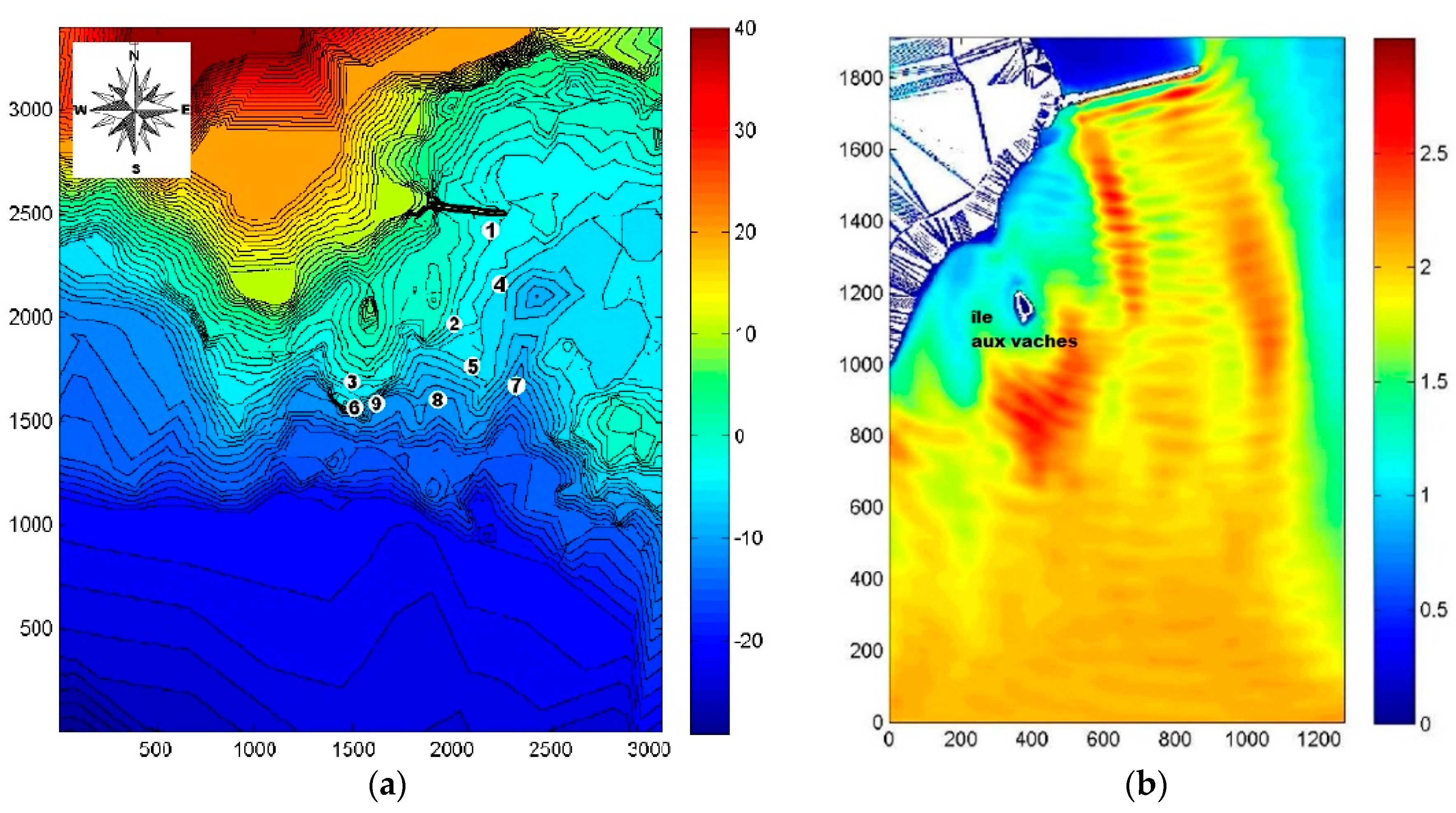
An in-deep examination of the Esquibien site characteristics allowed us to extract 9 relevant output points, as shown on the bathymetry illustration (see Figure 6a). These output points were chosen based on two criteria: alignment in front of the breakwater and water depth. Points 1, 2 and 3 lie in 3 m-depth, points 4, 5 and 6 in 5 m-depth and points 7, 8 and 9 in 10 m-depth. Points 3, 6 and 9 allow examining the depth influence on wave energy resource over a specific energetic area.
The reference simulation of Figure 6b uses the following wave conditions: significant wave height Hm0 = 2 m, peak period Tp = 12 s, wave direction θ = 200° N and a high tide water level of 4.75 m. The Swash simulation outputs are treated to produce maps of relevant wave parameters. The Hm0 map presents the main wave energy hot spots as the shoaling area in front of “île aux vaches”, corresponding to points 3, 6 and 9. In the western part of the map, close to point 4 and even closer to the breakwater (point 1), the significant wave height reached up to 2.7 m. In the eastern part of the map, wave heights 
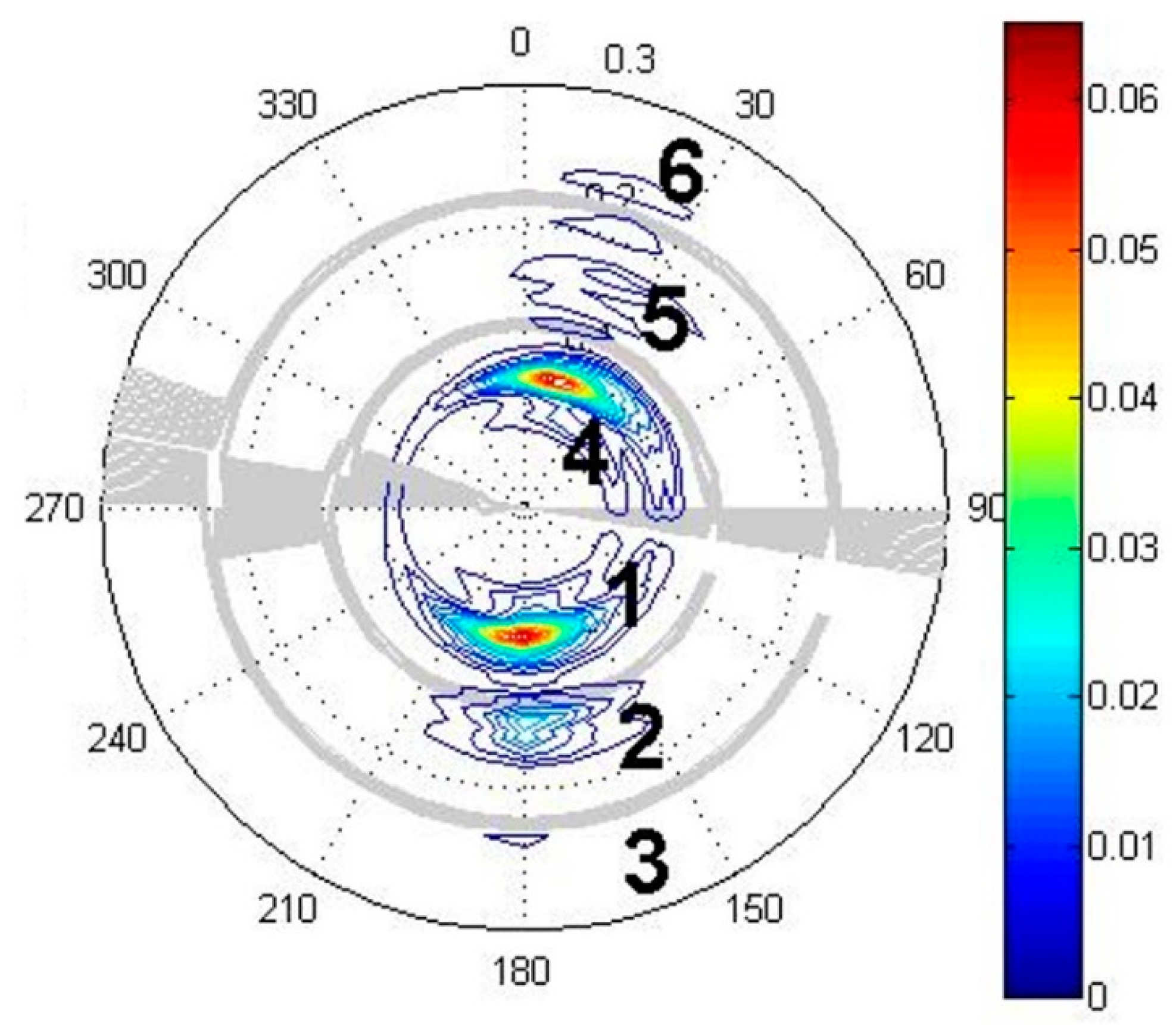
Hm0 less than 1.5 m are observed in a 6 m-deep area. At the tip of the breakwater, and at a regularly spaced distance, corresponding to half the wavelength, important wave height variations are evident. They are due to wave interferences responsible for the well-known standing wave phenomena characterized by nodes and anti-nodes at fixed locations. The obtained spectrum at point 1 in Figure 7 is represented in coordinates ( θ , f ) where θ is the wave direction, and f is the wave frequency. Figure 7 shows that the reflected wave keeps its peak period of 12 s. The available power is computed from the water surface elevation spectra, given the probabilities of occurrence of the various tidal levels and incoming wave conditions. It provides thus the total yearly energy at the point of interest. However, it should be noted that energy extraction devices are not all making exclusive use of heave at a single point. In addition, the location at Esquibien is the scene of reflection and shoaling effects that distribute the incoming energy into several categories, namely incident and reflected waves and primary free wave and harmonic bound waves at the sum and difference frequencies. When considering heave only, the incident and reflected waves may add or cancel as a function of the location, dominant wave direction and wavelength. A thorough design analysis will thus require to know how the energy can be split between those characteristics. To answer that question, this portioning analysis was carried out on the directional spectra for three tidal level conditions. This partitioning used a watershed algorithm [44,45] and resulted in 2 to 6 partitions depending on the location and conditions.
The characteristics of the partitions of Figure 7 are given in Table 5. From their directions, partitions 1–3 can be identified as an incident and partitions 4–6 as reflected. The incoming wave system is at period 12 s, and thus partitions 1 and 4 can be characterized as primary (free) waves, partitions 2 and 5 as harmonic, the sum of frequencies (bound) waves, and partitions 3 and 6 as superior order harmonics. When designing an energy extraction system, two points should be kept in mind. First, extraction of the incident power will decrease in proportion to the available reflected power unless the extent of the extraction system is narrow enough for waves to get around it and reflect; second, bound waves energy is difficult to extract, though some systems may benefit from the changes that they induce in the shape of the primary waves. It can be seen from Table 5 that the incident-free wave power, the only part that can be straightforwardly extracted, only amounts from one third to one half of the total observed power in a directional spectrum. Yet, since components from opposing directions may cancel, directional spectra usually exhibit more power than point heave spectra, as can be seen when comparing the two first columns of the table. Overall, the results indicate that the wave energy depends on the pair (Hm0, Tp) and on the water level that induced variations of the breakwater exposition, as seen in Table 6. At low tide, the “île aux vaches” shoal shelters the breakwater as it both focuses and dissipates energy through wave breaking. The breakwater is less exposed, as shown in the following maps of water surface elevation and significant wave height for the simulation at low tide. At high tide, the refraction weakens, and some areas become shoaling zones and make the breakwater more exposed. In Table 6, we name 0D the results with local Equation (2) and 2D with 2D Swash model.
The results of the 30 simulations at the 9 output points were gathered. Considering the probability density function of the tidal sea level, a sum was applied with the following weight coefficients—low tide (0.3), mid-tide (0.4), high tide (0.3)—in order to put together the 3 energy tables into a global yearly energy table. The yearly energy E and wave power P for the 9 output points of Esquibien, presented in Table 7, show power variations, P ranging from 9.3 to 20.8 kW/h depending on the location. Points 3, 6 and 9 can be compared because they lie in the same area (depth ranging from 3 to 10 m). There is not a strong impact of the water depth due to wave breaking on the power values at these points.
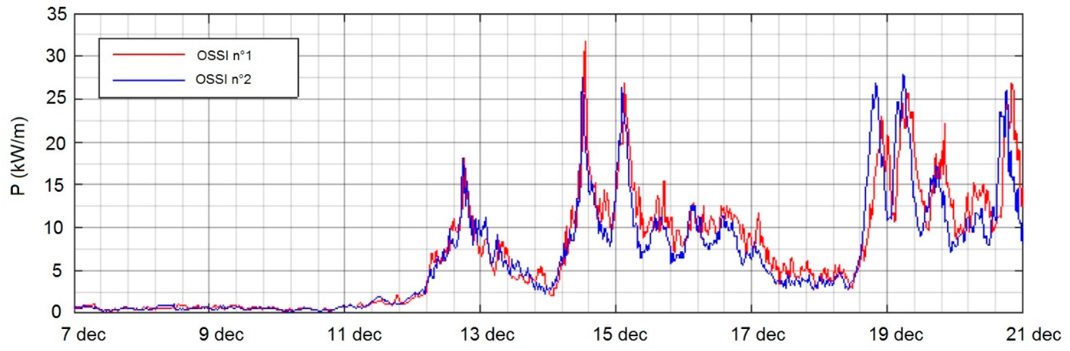
An observation campaign in 2013–2014 with two immersed pressure sensors from Ocean Sensor Systems, Inc. (OSSI) functioned from 7th of December 2013 to 3rd of March 2014 with sensor n° 1 (1 m LAT) located onshore and presented in Figure 8, and n° 2 (2 m LAT) located 100 m south. The average wave power that is observed onshore (OSSI n° 1) is 10% larger than the average wave power measured 100 m south (OSSI n° 2). That is due to the wave reflection on the breakwater. The results of the campaign are presented in Figure 9.
  • Saint-Guénolé
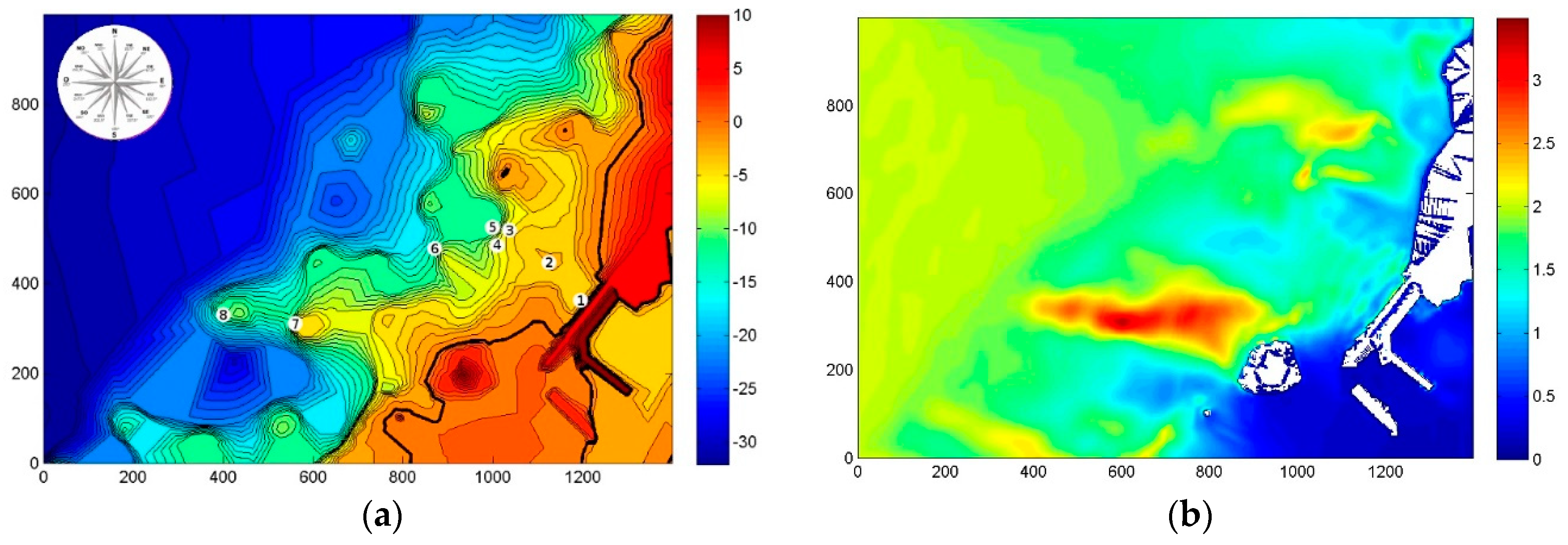
The reference simulation uses the following wave conditions: Hm0 = 2 m, Tp = 12 s, θ = 270° N and a mid-tide water level of 3.07 m.
The significant wave height map (Figure 10) shows that the wave energy is dramatically reduced by refraction and dissipation in the vicinity of the breakwater (3.1 kW/m at point 1). Conversely, the wave energy focuses in front of the rocky shoal at the southwest of the breakwater, with a wave power per unit crest length of 40.5 kW/m at output point 7. This feature is explained by the strong bottom slope that causes the waves to refract and to shoal in that region. This area is of great interest for wave energy converters (WEC) deployment, as the wave height exceeds 3 m over a 400 m distance. However, the wave energy is less directly in front of the breakwater with a wave height of only about 1.5 m and wave power per unit crest length of 10.2 kW/m at point 5. At low tide, the rocky shoal shelters the breakwater as it focuses and dissipates energy through wave breaking. The results for the yearly energy E and wave power P for the 8 output points of Saint-Guénolé, presented in Table 8, show power variations, P ranging from 2.4 at point 1 (located in front of the breakwater) to 33.6 kW/h at point 7, placed just off the steep rocky shoal. There is not a strong impact of the water depth due to wave breaking on the power values at four points 3 to 6 (water depth from 5 to 10 m) because, despite the variations of water depth, the wave power remains around 9 kW/m. Even at the 2 m-deep point 2, the wave power is still 6 kW/m. Points 7 and 8 are the most energetic points—their locations, near the shoal, in the southwest of the breakwater, favor wave-power focusing.

3.1.3. Bayonne and Saint-Jean-de-Luz

Two numerical simulations are run in the South of the Bay of Biscay in order to assess the wave power on the North breakwater of the port of Bayonne and on the Artha breakwater of Saint-Jean-de-Luz. Simulations consist of forcing a numerical wave model (Swan) with two different hindcast databases. The latter are, respectively, Anemoc [36] (EDF/LNHE et Cetmef; the period from 1979 to 2002; 23 years and 8 months) and Homere [38] (Ifremer; the period from 1994 to 2012; 18 years).
  • Saint-Jean-de-Luz
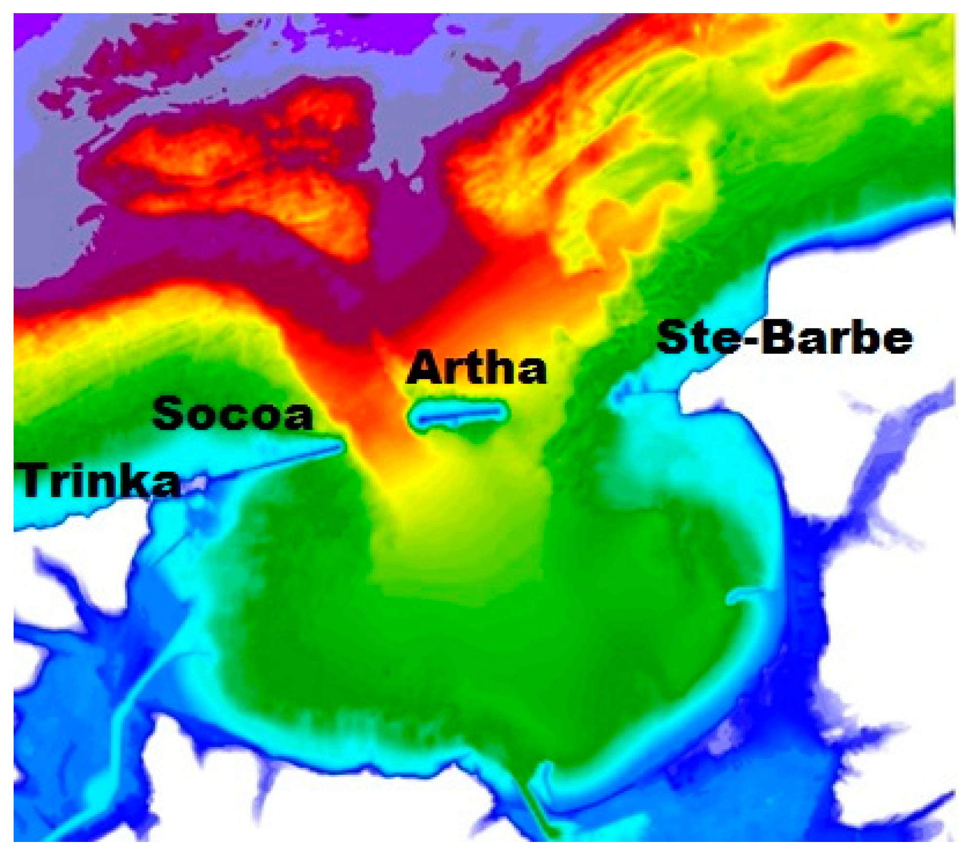
Located along the Gulf of Biscay, at 20 km East from the Spanish border, the Bay of Saint-Jean-de-Luz houses the cities of Saint-Jean-de-Luz, Ciboure and Urrugne. The bay is partially closed by three breakwaters from West to East: Socoa, Artha and Sainte-Barbe. Since the continental shelf is narrow in front of the bay, the waves are little dissipated, and the breakwaters frequently receive strong waves. The breakwaters were built between 1617 and 1895. Impacted by severe storms for many years, they were frequently repaired and reinforced. Almost every year, the breakwaters Artha and Socoa are reinforced by concrete armor units that have made after centuries a wide armor layer. The bathymetry is presented in Figure 11. The colors white, blue, to dark blue represent the areas that are constantly out of water. The areas in blue cyan represent the areas discovered at low tide. The remaining colors (green to red and purple) represent water depths up to 50 m.
Water depths in front of breakwaters vary from 0 to 18 m. The wave energy flow is calculated using data from the Anemoc base over 23.5 years. The wave propagation is simulated from the extraction points of the Anemoc database from the Basque coast to the coast of Saint-Jean-de-Luz. This provides information on the statistical wave characteristics near the site covering a long period, taking into account the tide and the bathymetry of the site. This simulation was carried out with the calculation code simulated wave nearshore (Swan)—Delft University of Technology [46].
Swan is a third-generation spectral wave model based on the conservation of the density of the wave action. It simulates the spread of sea states (wind seas and ocean waves) in the coastal domain. The model takes into account the effects of refraction and shoaling related to variations of bathymetry, diffraction by obstacles, wave generation by wind action, wave dissipation by breaking, bathymetric and friction on the bottom. The wave propagation is forced at the northern borders of the domain by the characteristics of the three-point waves at the northern border of the domain, in which the Anemoc database is available. At these points, the significant height of the Hs waves, their Tp period, the propagation direction and the directional range at the peak are known with a time step of 1 h. The time step of the model (one hour), fixed by the data of the Anemoc base, allows taking into account the tide. The change in water level over a year was calculated with the harmonic constituents of the tide using the FES2004 software [47]. The significant wave heights of the Anemoc database are compared with those of the result of the simulation by the Swan model at the three points. The comparison is for a 20-day duration. Swan model correctly propagates the wave forced by Anemoc to the borders of the domain. The average quadratic error lies between 13 cm and 33 cm. The main reasons why the results are slightly lower quality at one point are that the models used are different (Tomawac and Swan) and that for our simulation, wind patterns are not used. Since the propagation zone is large, the spread of the waves can be altered by the wind. However, the results remain of very good quality. They generate the wave calculated by the Swan model at the breakwater foot, results that we will present hereafter.
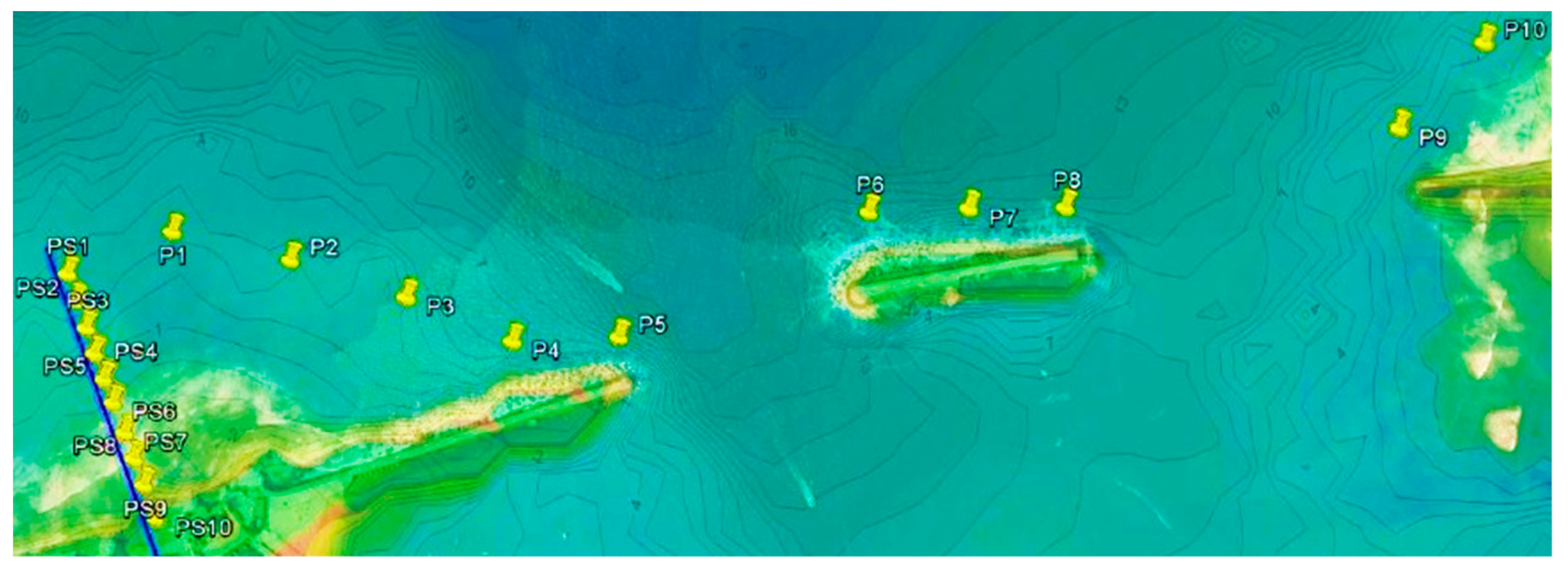
Considering the configuration of the bay, the breakwaters and the bathymetry, a series of ten points (P1 a P10) was defined on the isobath 4 m LAT along Socoa, Artha and Sainte Barbe (Figure 12). The depth of 4 m was chosen to ensure that the breakwater remains permanently submerged if a wave energy converter was placed there. This choice also allows the wave breaking to remain limited. The isobath 4 m is strongly moved away from the vicinity of Fort Socoa due to the rocky bottom that discovers the shore in front of the fort of Socoa at low tide. The points closest to the works are P4 a P9. A second series of ten points (PS1 to PS10) was placed along a perpendicular to the coast, in front of the Trinka. The points are equidistant between each other, and PS1 is also on the isobath 4 m LAT. Due to the configuration of the site and the heritage of the site, this site is considered to be one of the most appropriate to install a wave energy converter. This profile will also assess the impact of the choice of depth to install the wave energy converter.
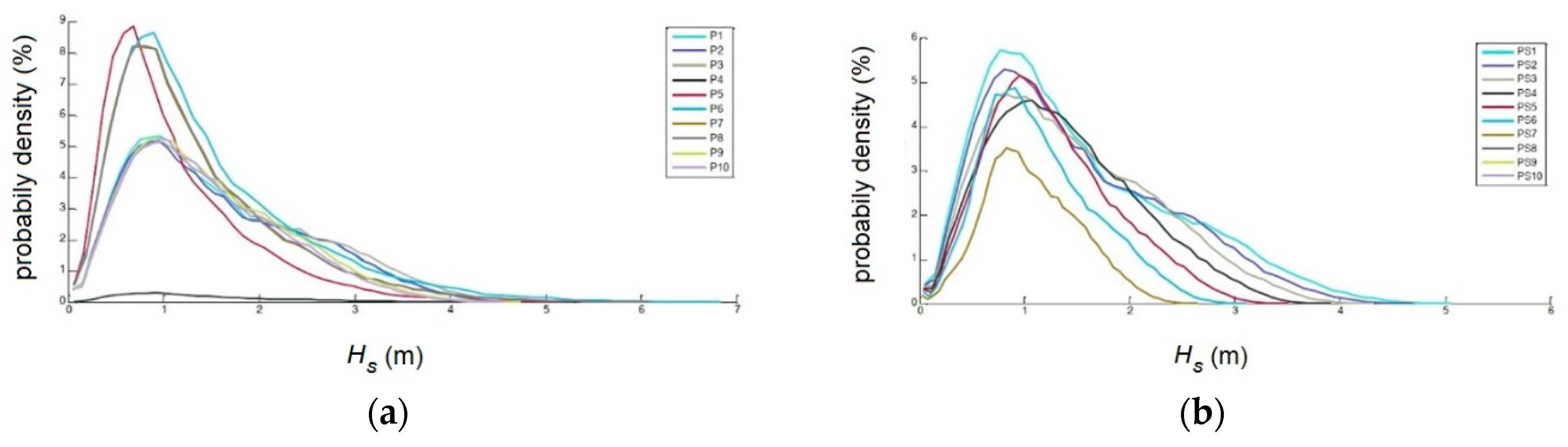
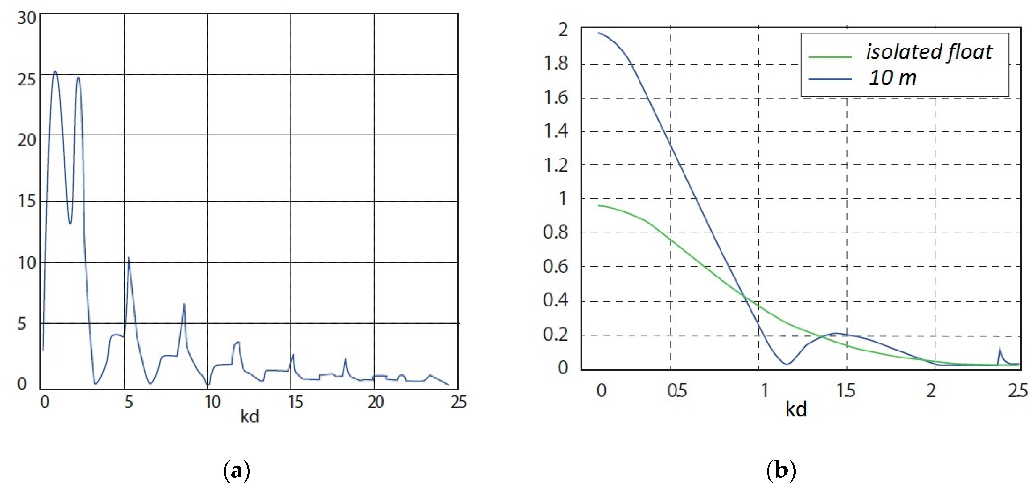
The laws of probabilities in Figure 13a show that large wave heights are more frequently recorded on the Artha breakwater (P6 a P7) and at the end of the Socoa breakwater (P5) than on Sainte-Barbe and Socoa. The water depth in these last points is the explanation. In the same way, we traced in Figure 13b the probabilities of annual occurrence at the points PS1 a PS10 on the cross-shore profile in front of Trinka breakwater. The strong attenuation of the wave heights results from bathymetric breaking. The simultaneous occurrence probabilities of a significant wave height Hs and a tidal water level Htidal are determined at different points on the site using the results of the Swan model forced by the Anemoc database. The results are expressed by defining classes of the significant wave height of the waves and of the tidal water level. 
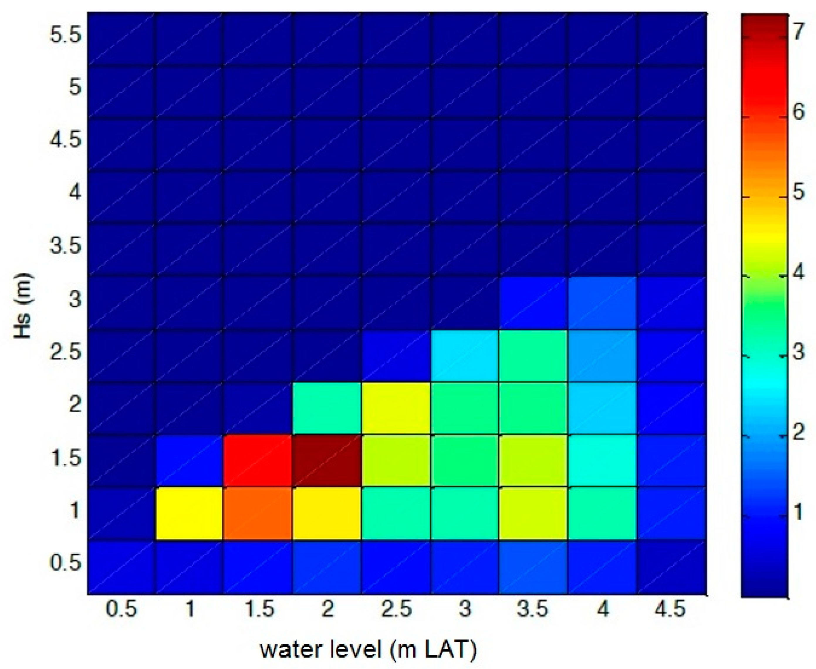
Figure 14 illustrates the most frequent classes at the point PS5. At low tide, the waves above 2 m no longer exist. At high tides, the highest waves do not exceed 3.5 m. The most frequent classes are centered around an average tide and wave heights between 0.5 and 2 m.
  • Bayonne
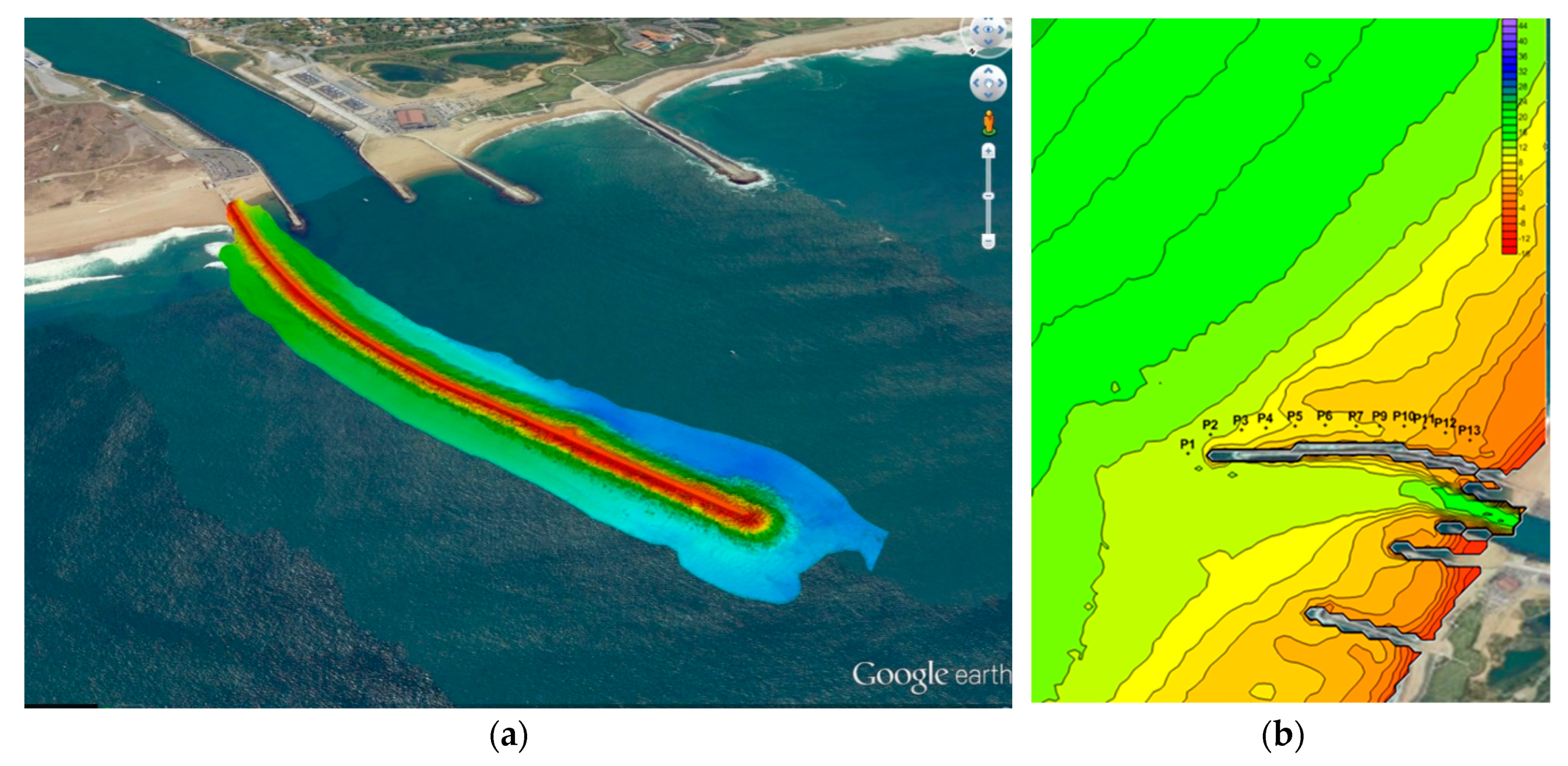
The implemented simulations allow us to calculate the wave propagation from offshore to onshore, using a model that is refined on the North breakwater of the port of Bayonne that is presented in 
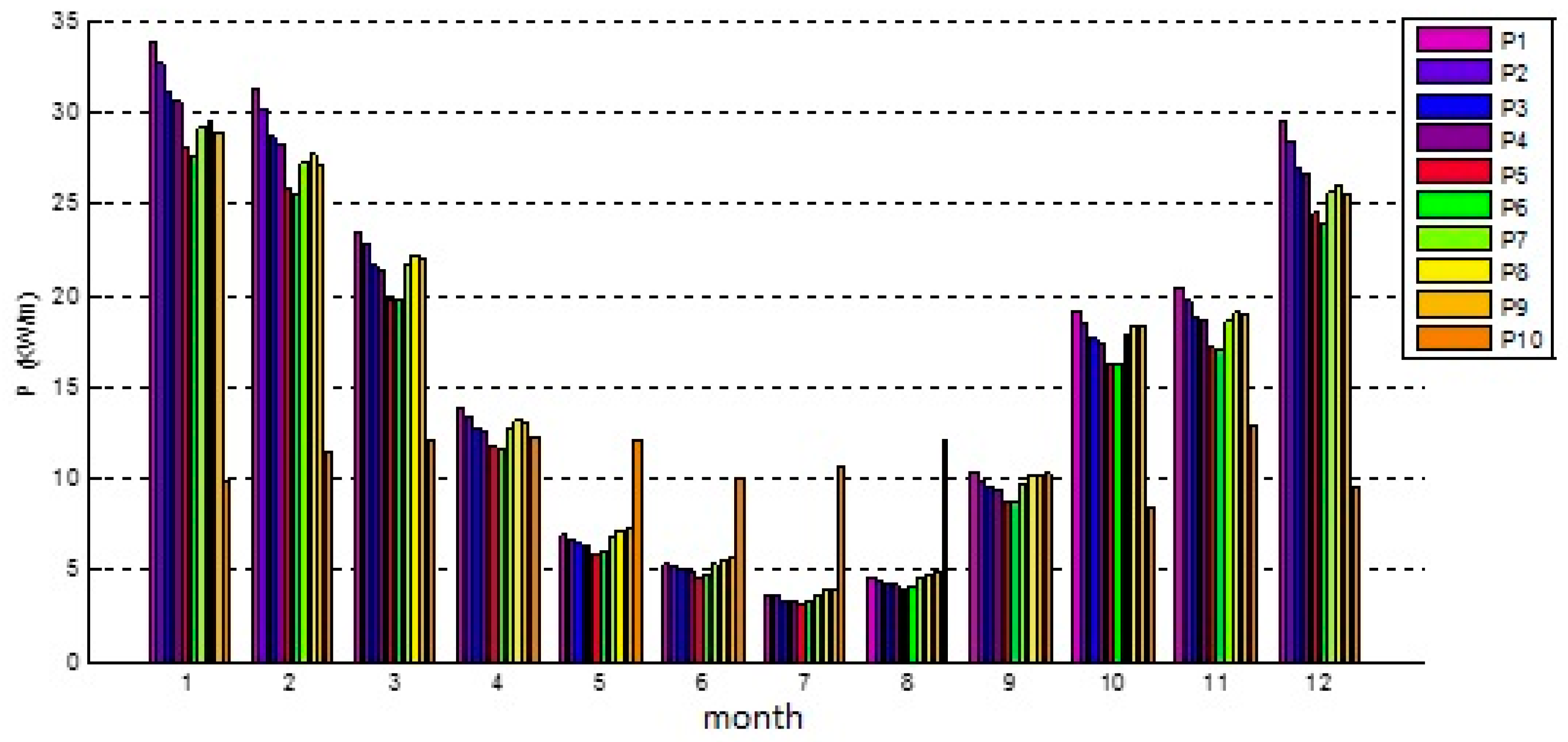
Figure 15a. High bathymetry resolution is taken into account, as well as the tidal phenomenon, which allows having a very good precision on the design of the wave energy converters. This method, which is costly in computation time, is an alternative to parametric formulas, much simpler to implement, but whose accuracy may be questioned for sites with complex bathymetry and subject to strong tidal range. First, a comparison of the results was carried out on offshore checkpoints. Great differences are observed between the “Swan Anemoc” in 
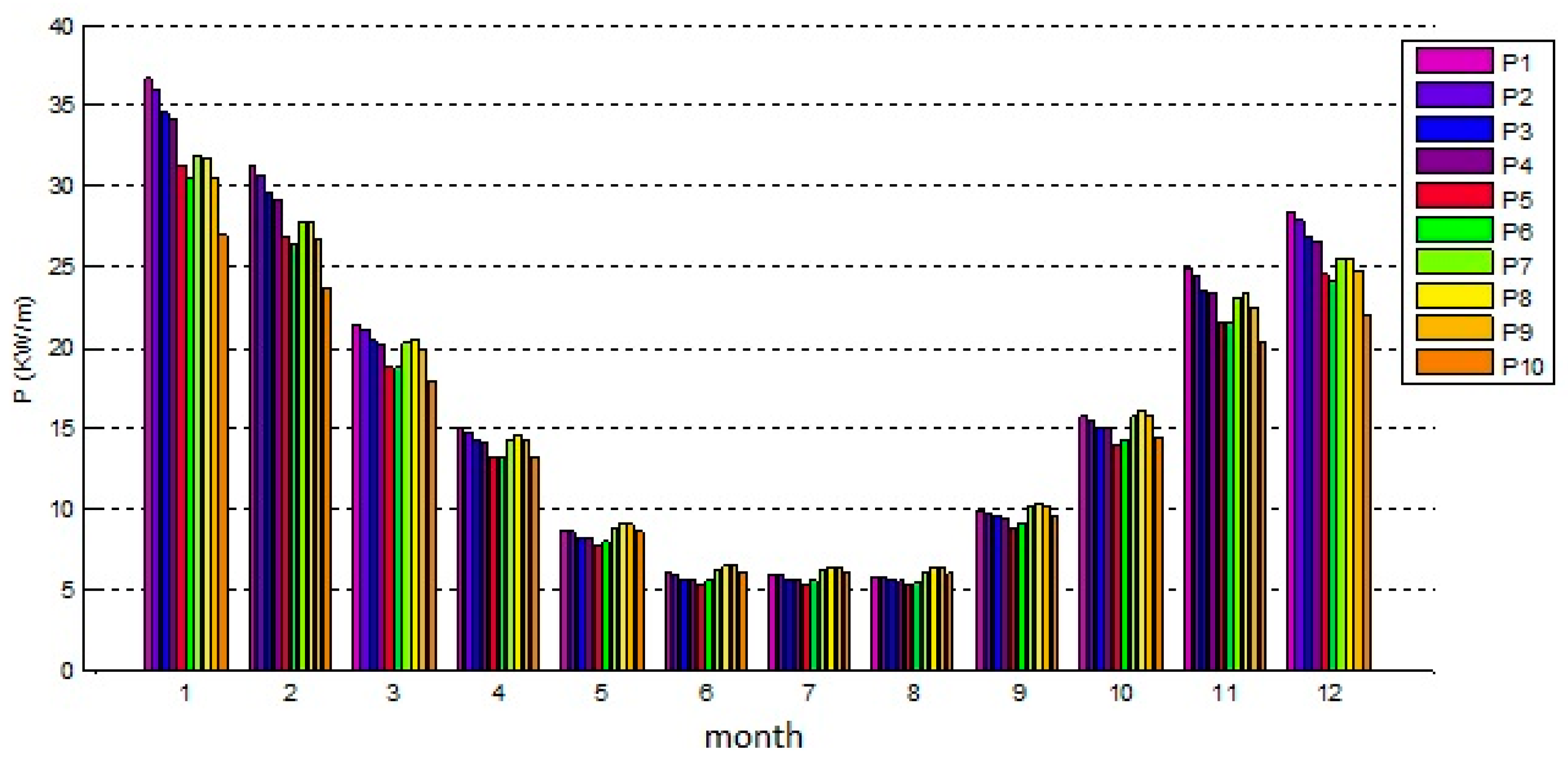
Figure 16 and the “Swan Homere” in Figure 17 with larger wave power in the winter months for the “Swan Anemoc”. Second, the comparison between the two simulations was made on 13 observation points located at the dike foot (see Figure 15b), on the north side, the most exposed to waves. Although significant differences are observed offshore, the differences in calculated power are weaker on the dike. In addition, the highest calculated power is given by the simulation forced by the Homere database.
As foreseen, the results present great differences between months in summer and months in winter. The ratio is up to 1 to 6. The results indicate that the annual average power is between 15 and 18 kW/m for the most offshore points and for the two databases. The power then drops sharply for the two points close to the coast. This average power of 15 to 18 kW/m is available over a length of approximately 650 m. In order to draw a parallel with the dikes of Saint-Jean-de-Luz, the energy available at the dike foot of Artha in Saint-Jean-de-Luz was around 14.2 kW/m on a maximum length of 250 m. The North breakwater of the port of Bayonne, therefore, represents an average power of 10.5 MW that is three times more important than the average power of 3.5 MW of Artha in Saint-Jean-de-Luz.

3.2. Calculation of the WEC Efficiency

The positioning of a wave power device oscillating in front of a dike must be carried out with care with regard to the values of the wavelength λ with respect to the distance L at which the device is placed from the vertical wall. We compare, in Figure 18, the amplitude of the response in pitch and heave of a flap oscillating and floating buoy, respectively, according to its distance d from the reflecting wall. Variations of the recovered power are also plotted. In both cases, we notice that the response amplitude operator (RAO) which is defined as the amplitude of the transfer function) include minimums for distances d, which are related to the position of the nodes and of the bellies of the standing wave produced in front of a reflective vertical wall. For the oscillating flap (Figure 18a), recent analytical studies [48] for a similar system show that the minima of the excitation torque are located in kd = mπ (wavenumber k, distance to the dike d). The position of these minima corresponds to the antinodes of the standing wave developed in front of the dike, where the horizontal component of the speed is zero. When the flap is placed at this point, it is no longer excited by the waves and the recovered power is canceled. This is confirmed in Figure 18a. For the oscillating float (Figure 18b), the vertical speed component is canceled out at the nodes of the standing wave in front of the wall, that is to say, in positions kd = (2 m + 1) π⁄2. When the buoy is placed at this point, the heave response and the recovered power cancel each other out. Figure 18 explains the advantage of placing a flap oscillating near a node of the standing wave, while the oscillating float should preferentially be placed near an antinode. It shows that the presence of the wall can considerably modify the recovery conditions of wave energy for the oscillating flap and the oscillating float. Table 9 confirms these results. For example, for the oscillating flap, when the distance to the dike is small and equal to 10 m, the power is multiplied by a factor of 2 in comparison with the case without the dike. However, when the distance is larger (30 m), the factor is just 1.
This illustration of the effect of the presence of a vertical dike behind the WEC was carried out in the theoretical case of a monochromatic wave, but the irregular wave simulations have shown that the distance to the dike criteria to optimize the power absorbed by the exposed WECs above remained valid for Jonswap spectra with shape parameter γ = 3.3. The site of Saint-Jean-de-Luz was chosen as an example first, to illustrate the capabilities of performance assessment tools. The wave power on this site was evaluated for a depth of 10 m, without taking into account the tide. The average annual powers that are evaluated for different distances to the dike for both types of WEC illustrate the need to place the device at an optimal distance depending on the operating principle of the WEC, as mentioned in the paragraph above and noted in [26]. Moreover, the average annual powers in Table 9 that are absorbed on the same site for isolated wave power systems, without dike, show the potential gain brought by an ideal vertical dike on the performance of the device wave power. In a case study, it will be essential to take into account the reflection coefficient of the dike, which will be at 75% better and which will necessarily reduce the energy performance of the device compared with the case of the ideal vertical dike presented here.

3.3. Cost of the kWh

3.3.1. Optimization of the System

For the overtopping systems, the number of reservoirs has a significant influence on the efficiency of the system. Overall, the more reservoirs are present; the more energy is produced. The economic optimum in Saint-Jean-de-Luz is obtained for four to five reservoirs. The cost of the kWh produced is reduced by 10% compared to a system with 3 reservoirs. An adaptation of the capacity of the turbines is searched as for classic hydroelectric systems. The influence on the cost of produced kWh is significant. A 30% reduction in equipment flow led to Saint-Jean-de-Luz at a 12% increase in the price per produced kWh. The optimum angle of the ramp is approximately 30°. The loss of efficiency is low for ramps angles between 25° and 35° and becomes significant when deviating from that range. The width of the reservoirs is adapted to the volume of water from waves producing the largest part of the power (apart from the extremes). A variation of 10 to 20% around this value has little influence on the cost of the produced kWh.
For the oscillating water columns, the design involves a product coefficient of wavenumber and water height in front of the opening. Pneumatic efficiency is a function whose maximum close to one coincides with a range of this coefficient between 1.2 and 1.5. The power that is absorbed by the system depends mainly on the movement of the water column and the air pressure inside the chamber if the room width is very smaller than the wavelength of incident waves. System optimization consists of identifying the range of the most energetic waves and setting the geometry of the system to be within the range of the most favorable kWh. The results in [29] and the example of the Mutriku water column allow a first approach of the dimensions to be adopted.
For the oscillating flaps, the values of the PTO parameters depend on the wave climate, and the tide controls the amplitude of oscillation of the flap because, beyond an angle of 40° (plus or minus 20° from the vertical), viscous effects significantly reduce the converted energy. The increase of the converted energy by optimizing the PTO parameters is around 5%. The oscillating flap must be ideally positioned at the vicinity of the nodes of the standing waves. The oscillating flap can, in theory, for a given wave period and, in the case of a totally reflective structure, achieve an efficiency close to 1.
For oscillating floats, optimization research leads to locate the system at the vicinity of antinodes of the standing waves. In practice, the floats are located near the dike. In addition, the optimization seeks to bring the resonance frequency of the system with that of the most energetic waves.

3.3.2. Efficiency of the System

The analyses on-site of Saint-Jean-de-Luz (incident wave power: 14 kW/m) and in Esquibien (incident wave power: 11 kW/m in point 1 and 16 kW/m in point 4) lead to the results in Table 10 with a fully reflecting breakwater:
SSG and OWC are not assessed in Esquibien. The efficiency of the oscillating flap and the oscillating float are much larger than SSG and OWC. With regard to oscillating flap and floating converters, the overall performance is, however, not valued. It will be taken into account in Table 11. The losses induced by the chain of electrical conversion are commonly evaluated at 30 to 50% of primary energy production. Table 11 shows the overall performance of the systems. The overall efficiency is defined as the ratio of the total power converted to electric power divided by the incident wave power on the dike width. For the active systems, the following assumptions are made: separation distance between active devices equal to the width of each of the units; reduction of 30 to 50% when converting to electricity; for the system with oscillating flap, a coefficient reducer of 0.74 to take into account the viscous effects; total reflection on the dike. For indication, from the documentation regarding the Wavestar project, the overall performance of this project to implement oscillating floats would be between 10 and 25%. Active systems of the oscillating flap and oscillating floats have the highest efficiency per linear meter. However, it is to qualify the statement considering that the wave reflection plays a significant role. The returns announced by the Wavestar project [49], however, confirm the results concerning the oscillating floats.

3.3.3. Cost of the System

The overtopping system. A 3D numerical model is set up in order to simulate the wave propagation and determine the pressure generated by its impact on the structure. A 3D numerical model is necessary because the structure is not completely two-dimensional. A view of the mesh of the finite element model is shown in Figure 19. Figure 20 shows the time variation of the average pressure on the structure. The greatest impact is recorded for the first wave. Estimated costs are based on the design, thus realized the various elements of the structure. Cost estimate for an overtopping structure in Saint-Jean-de-Luz led to the distribution presented in Figure 21a.
The oscillating column. Cost estimate for an oscillating column in Saint-Jean-de-Luz led to the distribution presented in Figure 21b.
The oscillating flap. The study of this type of system is carried out on the site of Artha (Saint-Jean-de-Luz). The entire system consists of 7 sections spaced of 20 m located in the profile of Figure 22. The cost estimate for an oscillating flap leads to the distribution in Figure 21c.
The oscillating float. The cost estimate for an oscillating float in Saint-Jean-de-Luz led distribution in Figure 21d.
Figure 21 presents the distribution of the cost. Construction costs include foundations, protections and modifications of the breakwater. Electro-mechanics costs include the system (for example, the flap or the float), the electric power converter and the power connection. Engineering costs represent studies and project management. The Table 12 shows the distribution of each item in the cost of the system as well as the cost per linear meter for the Saint-Jean-de-Luz site.

3.3.4. Production Costs

The following estimates are proposed to provide orders of magnitude and a first estimate of the comparative economic interest of devices. The Table 13 shows the fixed installation costs (CAPEX) of the various wave power systems presented and their main characteristics for a 60 m-long installation.
The Table 14 shows the LCoEs for the same systems with two discount rates.
This cost takes into account the initial investment, annual operation costs and maintenance costs (5% of the initial investment) as well as annual produced energy. It does not take into account the possible dismantling fees. All fluxes are converted to present value using a discount rate of 10%, then 7.5%, in order to guarantee the comparison with AIER data. The obtained results vary greatly depending on the considered system. With LCoEs greater than 1 euro/kWh, the overtopping systems and oscillating water columns are very uncompetitive in regards to other renewable energies. LCoE of the oscillating flaps and oscillating floats are consistent with the literature. Reduction of costs with the learning curve can make these technologies competitive. The potential French market only is composed of more than 180 km of dikes. As already mentioned, some companies already display LCoE much lower than our figures. We can, therefore, think that some cost reduction is already ongoing.

4. Conclusions

Onshore wave power systems, although relatively old, are not yet developed much around the world. However, they represent a strong interest for planners both in terms of the production of electrical energy and the protection against flooding. Electrification of ports to reduce pollutant emissions and the rise in sea levels with global warming have reinforced this interest.
Wave energy is highly seasonal energy with recoverable powers almost ten times greater in winter compared to summer. The power is expressed in kW/m. The converted energy will, therefore, depend on the length of the equipped dike. The dike cannot, in general, be equipped over its entire length due to multiple constraints, in particular with regard to bathymetry. Our assessment enabled us to select 20 study sites with high levels of wave power. Estimates of mean annual wave power levels vary from 0.9 kW/m at Belle-Ile up to 24 kW/m at Bayonne, and the lengths of useful dikes vary from 60 m at Molène, 500 m at Saint-Jean-de-Luz and up to 4000 m in Cherbourg. An in situ measurement campaign has shown that there is great uncertainty about the recoverable power due to the difficulties of both modeling and measuring in areas with sometimes reduced depths and disrupted bathymetries. At the operational level, it will be necessary to take into account regulatory, environmental and technical constraints in terms of soil analysis, electrical connection or energy storage depending on the mode of use of the selected energy production.
Among all the onshore wave power systems, four families stand out: overtopping systems, oscillating flaps, oscillating floats and oscillating water columns. The efficiency estimate shows that the wave reflection on the dike is an advantage in terms of energy production. Among the four families, we find that the oscillating flaps constitute the systems with the best returns. The design of the systems requires first to choose the converter, often called PTO, as power take-off and to size it. The systems can also be controlled in real time in order to continuously control the resistant forces to movement exerted by the PTO and therefore to increase the converted energy. Structural sizing then consists of evaluating the extreme stresses, evaluating the survivability of the system and defining safety strategies. A specific feature of WEC is the analysis of the stress on the supporting structure and the potential hydrosedimentary impact.
Finally, we have introduced the concept of levelized cost of energy (LCoE), which relates the costs generated by the installation to the energy produced throughout its life cycle. LCoE expresses the cost of energy in euros/kWh. This analysis carried out for the four families of wave power systems showed that the float systems had the lowest LCoE (around 0.3 €/kWh), followed closely by the oscillating flaps. As expected, oscillating water columns and overtopping systems have nearly five times these LCoEs. Oscillating floats and oscillating flaps can therefore propose costs close to other renewable energies such as solar and wind power. Even if the cost of renewable energies decreases for each technology, we can expect the cost of onshore wave power systems to decrease faster as the number of units produced increases. In addition, it can be considered to concentrate the wave in front of these systems in order to increase electricity production and further reduce the LCoE.
The economic analysis should not overlook the dual vocation that we envisage for these developments: production of electricity and the protection against flooding. Onshore wave power systems thus participate in two strategies to respond to climate change: the first is mitigation by contributing to the production of renewable energy, and the second is adaptation by reducing the consequences of sea-level rise like wave overtopping, structural damages and sand erosion.

Funding

This research was funded by the French national project EMACOP in the framework of the RGCU (Réseau Génie Civil et Urbain).

Conflicts of Interest

The authors declare no conflict of interest.

References

  1. Clément, A.; McCullen, P.; Falcão, A.; Fiorentino, A.; Gardner, F.; Hammarlund, K.; Lemonis, G.; Lewis, T.; Nielsen, K.; Petroncini, S.; et al. Wave energy in Europe: Current status and perspectives. Renew. Sustain. Energy Rev. 2002, 6, 405–431. [Google Scholar] [CrossRef]
  2. Falcao, A.F.O. Wave energy utilization: A review of the technologies. Renew. Sustain. Energy Rev. 2010, 14, 899–918. [Google Scholar] [CrossRef]
  3. Cerema. Systèmes Houlomoteurs Bords à Quai: Guide de Conception en Phase Avant Projet; Editions Cerema: Bron, France, 2020; ISBN 978-2-37180-427-2. [Google Scholar]
  4. Babarit, A.; Hals, J.; Muliawan, M.; Kurniawan, A.; Moan, T.; Krokstad, J. Numerical benchmarking study of a selection of wave energy converters. Renew. Energy 2012, 41, 44–63. [Google Scholar] [CrossRef]
  5. Brito-Melo, A. Modélisation de la Centrale Européenne a Énergie des Vagues sur l’île de Pico, Açores. Ph.D. Thesis, University of Nantes, Nantes, France, 2000. [Google Scholar]
  6. Falcao, A.F.O.; Henriques, J.C.C. Model-prototype similarity of oscillating water column wave energy converters. Int. J. Mar. Energy 2014, 6, 18–34. [Google Scholar] [CrossRef]
  7. Delauré, Y.; Lewis, A. 3D hydrodynamics modelling of a fixed oscillating water column wave power plant by a boundary element method. Ocean Eng. 2003, 30, 309–330. [Google Scholar] [CrossRef]
  8. Soares, C.G.; Bento, A.R.; Goncalves, M.; Silva, D.; Martinho, P. Numerical evaluation of the wave energy resource along the Atlantic European coast. Comput. Geosci. 2014, 71, 37–49. [Google Scholar] [CrossRef]
  9. Pastor, J.; Liu, Y. Wave climate resource analysis for deployment of wave energy conversion technology. Sustainability 2016, 8, 1321. [Google Scholar] [CrossRef] [Green Version]
  10. Pastor, J.; Liu, Y. Wave energy conversion and its renewable energy potential for the oil and gas industry. In Proceedings of the Industrial Energy Technology Conference, New Orleans, LA, USA, 20–23 May 2014. [Google Scholar]
  11. Pastor, J.; Liu, Y. Hydrokinetic energy overview and energy potential for the Gulf of Mexico. In Proceedings of the IEEE Green Technologies Conference, Tulsa, OK, USA, 19–20 April 2012. [Google Scholar]
  12. Guiberteau, K.L.; Liu, Y.; Lee, J.; Kozman, T.A. Potential of development and application of wave energy conversion technology in the Gulf of Mexico. In Proceedings of the Industrial Energy Technology Conference, New Orleans, LA, USA, 20–23 May 2014. [Google Scholar]
  13. Guillou, N.; Chapalain, G. Wave energy potential in the Sea of Iroise. In Proceedings of the 11th European Wave and Tidal Energy Conference Series, Nantes, France, 6–11 September 2015. [Google Scholar]
  14. Biyela, S. Techno-economic analysis framework for wave energy conversion schemes under South African conditions: Modeling and simulations. In Proceedings of the 18th International Conference on Renewable Energy Resources and Application, Belfort, France, 8–10 February 2016. [Google Scholar]
  15. Babarit, A. Contribution à la Récupération de l’Énergie des Vagues. Ph.D. Thesis, Université de Nantes, Nantes, France, 2016. [Google Scholar]
  16. International Renewable Energy Agency (IRENA). Ocean Energy: Technology Readiness, Patents, Deployment Status and Outlook; International Renewable Energy Agency (IRENA): Abu Dhabi, UAE, 2014. [Google Scholar]
  17. Goda, Y. Deformation of irregular waves due to depth-controlled wave breaking. Rep. Port Harb. Res. Inst. 1975, 14, 59–106. [Google Scholar]
  18. Electric Power Research Institute (EPRI). Mapping and Assessment of the United States Ocean Wave Energy Resource; EPRI Technical Report; Electric Power Research Institute (EPRI): Palo Alto, CA, USA, 2011; 176p. [Google Scholar]
  19. Bishop, C.T.; Donelan, M.A. Measuring waves with pressure transducers. Coast. Eng. 1987, 11, 309–328. [Google Scholar] [CrossRef]
  20. Kofoed, J.P. Wave Overtopping of Marine Structures—Utilization of Wave Energy. Ph.D. Thesis, Aalborg University, Aalborg, Denmark, 2002. [Google Scholar]
  21. Van der Meer, J.W.; Jansen, J.F.P.M. Wave Run-Up and Wave Overtopping at Dikes; Technical Report; In Task Committee Reports; American Society of Civil Engineers (ASCE): Reston, VA, USA, 2002. [Google Scholar]
  22. Babarit, A.; Delhommeau, G. Theoretical and numerical aspects of the open source BEM solver NEMOH. In Proceedings of the European Wave and Tidal Energy Conference (EWTEC), Nantes, France, 6–11 September 2015. [Google Scholar]
  23. Delhommeau, G. Seakeeping codes Aquadyn and Aquaplus. In Proceedings of the 19th WEGEMT School, Numerical Simulation of Hydrodynamics: Ships and Offshore Structures, Nantes, France, 20–24 September 1993. [Google Scholar]
  24. Penalba, M.; Ringwood, J.V. A review of wave to wire models for wave energy converters. Energies 2016, 9, 506. [Google Scholar] [CrossRef] [Green Version]
  25. Meunier, P.M. Contrôle Collaboratif d’une Ferme de Génératrices Houlomotrices. Ph.D. Thesis, Ecole Centrale de Nantes, Nantes, France, 2018. [Google Scholar]
  26. Baudry, V.; Marrone, S.; Babarit, A.; le Touzé, D.; Clément, A.H. Power matrix assessment and extreme loads estimation on a flap-type wave energy converter in front of a dike. In Proceedings of the European Wave and Tidal Energy Conference, Nantes, France, 6–11 September 2015. [Google Scholar]
  27. Evans, D.V. The oscillating water column wave energy device. J. Inst. Maths Appl. 1978, 22, 423–433. [Google Scholar] [CrossRef]
  28. Delauré, Y.M.C.; Lewis, A. A 3D Parametric Study of a rectangular Bottom-Mounted OWC power plant. In Proceedings of the 11th ISOPE Conference, Stavanger, Norway, 17–22 June 2001. [Google Scholar]
  29. Zhang, Y.; Zou, Q.P.; Greaves, D. Air-Water two phase modelling of hydrodynamic performance of an oscillating water column device. Renew. Energy 2012, 41, 159–170. [Google Scholar] [CrossRef]
  30. Itturioz, A.; Guanche, R.; Armesto, J.A.; Alves, M.A.; Vidal, C.; Losada, I.J. Time-domain modeling of a fixed detached oscillating water column towards a floating multi-chamber device. Ocean Eng. 2014, 76, 65–74. [Google Scholar] [CrossRef]
  31. Rameliarison, V.; Astruc, D.; Chapalain, G. Assessment of Navier-Stokes modelling of an Oscillating Water Column wave energy converter. In Proceedings of the European Wave and Tidal Energy Conference, Nantes, France, 6–11 September 2015. [Google Scholar]
  32. Karmath, A.; Bihs, H.; Arntsen, O.A. Numerical modeling of power take off damping in an oscillating water column device. Int. J. Mar. Energy 2015, 10, 1–16. [Google Scholar] [CrossRef] [Green Version]
  33. Babarit, A.; Hals, J. On the maximum and actual capture width ratio of wave energy converters. In Proceedings of the European Wave and Tidal Energy Conference, Southampton, UK, 5–9 September 2011. [Google Scholar]
  34. Benoit, M.; Lafon, F.; Goasguen, G. Constitution et exploitation d’une base de données d’états de mer le long des côtes françaises par simulation numérique sur 23 ans. Base ANEMOC en Atlantique, Manche et Mer du Nord. Eur. J. Environ. Civ. Eng. 2008, 12, 35–50. [Google Scholar] [CrossRef]
  35. Scilab. Available online: http://www.scilab.org (accessed on 14 December 2017).
  36. Mattarolo, G.; Benoit, M.; Lafon, F. Wave energy resource off the French coasts: The Anemoc database applied to the energy yield evaluation of Wave Energy Converters. In Proceedings of the 8th European Wave and Tidal Energy Conference (EWTEC 2009), Uppsala, Sweden, 7–10 September 2009. [Google Scholar]
  37. Suzuki, T.; Verwaest, T.; Hassan, W.; Veale, W.; Reyns, J.; Trouw, K.; Troch, P.; Zijlema, M. The applicability of SWASH model for wave transformation and wave overtopping: A case study for the Flemish coast. In Proceedings of the 5th International Conference on Advanced COmputational Methods in ENgineering (ACOMEN 2011), Liège, Belgium, 14–17 November 2011; pp. 1–11. [Google Scholar]
  38. Homere. Available online: http://www.previmer.org/en/produits/hindcast_sea_states_homere (accessed on 14 December 2017).
  39. Blue Kenue. Available online: http://www.nrccnrc.gc.ca/eng/solutions/advisory/blue_kenue_index.html (accessed on 14 December 2017).
  40. Boudiere, E.; Maisondieu, C.; Ardhuin, F.; Accensi, M.; Pineau-Guillou, L.; Lepesqueur, J.A. Suitable metocean hindcast database for the design of Marine energy converters. Int. J. Mar. Energy 2013, 3-4, 40–52. [Google Scholar] [CrossRef] [Green Version]
  41. Wafo. Available online: http://www.maths.lth.se/matstat/wafo/ (accessed on 14 December 2017).
  42. Diswap. Available online: http://www.metocean.co.nz/support/resources/ (accessed on 14 December 2017).
  43. Zijlema, M.; Stelling, G.; Smit, P. SWASH: An operational public domain code for simulating wave fields and rapidly varied flows in coastal waters. Coast. Eng. 2011, 58, 992–1012. [Google Scholar] [CrossRef]
  44. Hanson, J.L.; Phillips, O.M. Automated analysis of ocean surface directional wave spectral. J. Atmos. Ocean. Technol. 2001, 18, 277–293. [Google Scholar] [CrossRef]
  45. Portilla, J.; Ocampo-Torres, F.J.; Monbaliu, J. Spectral partitioning and identification of wind sea and swell. J. Atmos. Ocean. Technol. 2009, 26, 107–122. [Google Scholar] [CrossRef]
  46. Swan. Available online: http://www.swan.tudelft.nl/ (accessed on 14 December 2017).
  47. FES2004. Available online: http://www.legos.obs-mip.fr/produits/soa/niveau-de-la-mer-maree/modele-global-de-maree-fes) (accessed on 14 December 2017).
  48. Sarkar, D.; Renzi, E.; Dias, F. Wave power absorption from a flap-type wave energy converter near a straight coast. In Proceedings of the European Wave and Tidal Energy Conference, Aalborg, Denmark, 2–5 September 2013. [Google Scholar]
  49. Frigaard, P.B.; Andersen, T.L.; Kofoed, J.P.; Kramer, M.M.; Ambühl, S. Wavestar Energy Production Outlook; Aalborg University Report; Aalborg University: Aalborg, Denmark, 2016. [Google Scholar]
Figure 1. The four families of wave energy converters: (a) overtopping system, (b) oscillating water column, (c) oscillating flap, (d) oscillating float.
Jmse 08 00947 g001
Figure 2. Cross-section of an overtopping system reproduced with permission from Cerema “Systèmes houlomoteurs bords à quai, guide de conception en phase avant projet” published by Cerema (2020) [3].
Jmse 08 00947 g002
Figure 3. Modeling principle of the front flap a totally reflective vertical dike through symmetry reproduced with permission from Cerema “Systèmes houlomoteurs bords à quai, guide de conception en phase avant projet” published by Cerema (2020) [3].
Jmse 08 00947 g003
Figure 4. Planar piston (a) and distribution of pressure (b) reproduced with permission from Cerema “Systèmes houlomoteurs bords à quai, guide de conception en phase avant projet” published by Cerema (2020) [3].
Jmse 08 00947 g004
Figure 5. Location of the 20 sites along the French coast.
Jmse 08 00947 g005
Figure 6. Esquibien (a) bathymetry map and location of the 9 output points; (b) significant wave height (m) for the reference simulation.
Jmse 08 00947 g006
Figure 7. Results of partitioning at point 1 for the reference simulation.
Jmse 08 00947 g007
Figure 8. Pressure sensor OSSI n°1 in Esquibien.
Jmse 08 00947 g008
Figure 9. Results of the campaign 2013–2014 in Esquibien with two pressure sensor OSSI.
Jmse 08 00947 g009
Figure 10. Saint-Guénolé (a) bathymetry map and location of the 8 output points; (b) significant wave height (m) for the reference simulation.
Jmse 08 00947 g010
Figure 11. Bathymetry of Bay of Saint-Jean-de-Luz.
Jmse 08 00947 g011
Figure 12. Control points in the vicinity of the breakwaters of Saint-Jean-de-Luz.
Jmse 08 00947 g012
Figure 13. (a) Probability density in the points P1 to P10 along the Artha, Socoa and Saint-Barbe breakwater (b) Probability density in the points PS1 to PS10 along the cross-shore profile of Trinka breakwater.
Jmse 08 00947 g013
Figure 14. Annual occurrences in% (from 0% in dark blue to 7% in dark red) of classes (wave height/tidal water level) at point PS5.
Jmse 08 00947 g014
Figure 15. (a) Location of Bayonne North breakwater and (b) locations of the 13 observation points.
Jmse 08 00947 g015
Figure 16. Monthly average wave power at the Bayonne site on 10 observation points simulated with Anemoc database.
Jmse 08 00947 g016
Figure 17. Monthly average wave power at the Bayonne site on 10 observation points simulated with Homere database.
Jmse 08 00947 g017
Figure 18. (a): RAO recovered by an oscillating flap as a function of kd the product of the wavenumber k and of the distance to the dike d. (b): RAO recovered by an oscillating float. Comparison between a buoy placed 10 m from the dike (blue) and an isolated buoy (green).
Jmse 08 00947 g018
Figure 19. Mesh of the finite element model with dimensions.
Jmse 08 00947 g019
Figure 20. Time variation of the average pressure on the structure.
Jmse 08 00947 g020
Figure 21. Distribution of cost (€–2017) for the addition of a wave energy converter (WEC) to the breakwater of Saint-Jean-de-Luz with construction costs in blue, electro-mechanics in red and engineering in green.
Jmse 08 00947 g021
Figure 22. Example of hydraulic converter for Oyster project reproduced with permission from Cerema “Systèmes houlomoteurs bords à quai, guide de conception en phase avant projet” published by Cerema (2020) [3].
Jmse 08 00947 g022
Table 1. Offshore results and data for 20 sites.
SiteN° Point AnemocDepth (m LAT)Distance to Shore (km)Annual Mean Wave Power (kW/m)Winter Mean Wave Power (kW/m)Summer Mean Wave Power (kW/m)Annual mean Wave Height (m)Energy Mean Period Te (s)Mean Wave Direction (°/North)
Boulogne sur mer134158102.94.41.40.85.7250
Antifer189043404.97.82.216.2280
Cherbourg115464249.314.54.11.36.850; 270
Flamanville2291352014.223.25.41.57.8270
Roscoff1080661027.743.81228.8285
Molène0730801020.130.69.81.88.3300
Le Conquet0398973054.188.020.82.69.1285
Esquibien1232603044.371.118.02.49.0285
Saint-Guénolé1232603044.371.118.02.49.0285
Lesconil02811004044.270.618.32.49.1280
Groix415011512.219.83.51.29.6225
Quiberon0874723623.538.19.21.79.0260
Belle-île2421321211.218.44.10.99.0250
Le Croisic1499503820.633.18.31.69.1260
L’Herbaudière1544513529.046.911.51.99.4275
Saint-Gilles-Croix-de-Vie03151036534.655.114.42.19.3275
Les Sables d’Olonne03151036534.655.114.42.19.3275
La Cotinière1105654428.344.812.11.99.2275
Bayonne0016198825.840.411.41.810.1300
Saint-Jean-de-Luz0016198825.840.411.41.810.1300
Table 2. Onshore results and data for 20 sites.
SiteDepth
(m LAT)
Mean Sea Level (m)Annual Mean Wave Power (kW/m)Winter Mean Wave Power (kW/m)Summer Mean Wave Power (kW/m)Annual Mean Wave Height (m)
Hc
Mean Wave Direction (°/North)Length of Useful Structure (m)
Boulogne sur mer34.92.84.21.30.72601600
Antifer164.95.18.22.20.92801900
Cherbourg103.84.46.32.5160; 3004000
Flamanville35.413.622.25.41.4270700
Roscoff25.37.810.84.91.20; 40300
Molène04.37.911.64.81.334560
Le Conquet14.021.130.211.82.1250140
Esquibien23.16.98.43.41.3140340
Saint-Guénolé23.021.130.212.62.1285250
Lesconil03.18.19.75.21.5190200
Groix13.1XXXXX200
Quiberon03.15.88.23.21.1210350
Belle-Île23.10.91.00.70.525; 100200
Le Croisic−23.31.61.91.40.8315450
L’Herbaudière−23.41.82.11.60.9325100
Saint-Gilles-Croix-de-Vie13.212.217.96.61.6240250
Les Sables d’Olonne13.210.313.45.11.4210100
La Cotinière−23.62.53.11.91.0225150
Bayonne72.524.337.811.11.8300500
Saint-Jean-de-Luz102.521.833.810.11.6315500
Table 3. Occurrences of the (Hm0, Tp) pairs in hours/year.
Tp (s)5–77–99–1111–1313–1515–17
Hm0 (m)
5.5–6.50.00.00.25.021.628.7
4.5–5.50.00.13.941.078.073.3
3.5–4.50.06.543.0130.0203.1107.3
2.5–3.52.975.1139.7316.8351.9123.8
1.5–2.595.8306.7423.0782.7493.9116.9
0.5–1.5243.3862.21348.61228.4360.0111.1
0.0–0.520.3169.5155.762.618.56.9
Table 4. The 10 (Hm0, Tp) pairs were selected to represent the Esquibien wave climate.
Tp (s)8101214
Hm0 (m)
3 XXX
2XXXX
1XXX
Table 5. Split-out evaluation of the potential wave power in kW/m for a 2 m-high wave incoming at high tide (total wave power of 22.37 kW/m).
Wave ParametersIncident Wave SystemsReflected Wave Systems
System 1System 2System 3System 4System 5System 6
Hm0 (m)1.270.690.231.240.510.26
Tp (s)12.636.244.1012.425.774.08
P (kW/m)8.832.580.298.351.390.38
Table 6. Incident and reflected wave power in kW/m at low tide, mid-tide and high tide.
Water LevelTotal Power (0D)Total Power (2D)Incident FreeReflected Free
Low tide (1.45 m)10.1613.434.894.99
Mid-tide (3.07 m)16.7219.589.417.15
High tide (4.75 m)16.3022.378.838.35
Table 7. Results for the yearly energy E (MWh/m) and wave power P (kW/m) in each of the 9 output points in Esquibien.
Output Point123456789
Yearly E (MWh/m)99.981.9135.9137.4123.4174.483.8176.2181.9
P (kW/m)11.49.315.515.714.119.99.620.120.8
Table 8. Results for the yearly energy E (MWh/m) and wave power P (kW/m) in each of the 8 output points in Saint-Guénolé.
Output Point12345678
Yearly E (MWh/m)20.952.276.973.082.877.2294.1209.8
P (kW/m)2.46.08.88.49.48.833.623.9
Table 9. Absorbed power in Saint-Jean-de-Luz according to the distance to the dike.
Without Diked = 10 md = 15 md = 30 m
Produced power (kW)Oscillating float2653x26
Oscillating flap150x320349
Table 10. Hydrodynamic efficiency in Saint-Jean-de-Luz and Esquibien (* point 4 and ** 1).
Overtopping System (SSG)Oscillating Water Column (OWC)Oscillating FlapOscillating Float
Absorbed power (kW/m)Saint-Jean-de-Luz2–3.32.813.26.0
Esquibienxx9.7 *6.1 **
Efficiency (%)Saint-Jean-de-Luz15209443
Esquibienxx62 *54 **
Table 11. Global efficiency in two sites (Saint-Jean-de-Luz and Esquibien in two different locations with * point 4 and ** 1 of Figure 2).
Overtopping System (SSG)Oscillating Water Column (OWC)Oscillating FlapOscillating Float
Produced power (kW/m)Saint-Jean-de-Luz1.20.82.4–3.41.5–2.1
Esquibienxx1.8–2.5 *1.5–2.1 **
Efficiency (%)Saint-Jean-de-Luz8.56–6.517–2411–15
Esquibienxx11–16 *13–19 **
Table 12. Distribution and cost of systems per linear meter.
Overtopping System (SSG)Oscillating Water Column (OWC)Oscillating FlapOscillating Float
Construction66%72%30%37%
Electromechanics26%19%62%55%
Engineering8%8%8%8%
Cost by meter119 k€100 k€80 k€35 k€
Table 13. Fixed installation costs (CAPEX) of the four 60 m-long systems in Saint-Jean-de-Luz.
Power (kW/m)SiteDescriptionCost of the System (k€)
Overtopping system (SSG)1.2–1.7Socoaa 60 m-long structure7150
Oscillating water column (OWC)0.8–1Socoaa 60 m-long structure5850
Oscillating flap3–3.5ArthaTwo 20 m-wide flaps4800
Oscillating float1.5–2.1ArthaThree buoys with a diameter of 10 m1880
Table 14. Levelized costs of energy (LCoEs) of the four 60 m-long systems.
Levelized Cost of Energy (euro/kWh); r = 10%Levelized Cost of Energy (euro/kWh); r = 7.5%
Overtopping system (SSG)1.77–1.251.52–1.05
Oscillating water column (OWC)2.17–1.731.87–1.50
Oscillating flap0.47–0.400.41–0.35
Oscillating float0.37–0.270.32–0.23
Publisher’s Note: MDPI stays neutral with regard to jurisdictional claims in published maps and institutional affiliations.

