A Fast Algorithm for the Prediction of Ship-Bank Interaction in Shallow Water

Abstract

The hydrodynamic interaction induced by the complex flow around a ship maneuvering in restricted waters has a significant influence on navigation safety. In particular, when a ship moves in the vicinity of a bank, the hydrodynamic interaction forces caused by the bank effect can significantly affect the ship’s maneuverability. An efficient algorithm integrated in onboard systems or simulators for capturing the bank effect with fair accuracy would benefit navigation safety. In this study, an algorithm based on the potential-flow theory is presented for efficient calculation of ship-bank hydrodynamic interaction forces. Under the low Froude number assumption, the free surface boundary condition is approximated using the double-body model. A layer of sources is dynamically distributed on part of the seabed and bank in the vicinity of the ship to model the boundary conditions. The sinkage and trim are iteratively solved via hydrostatic balance, and the importance of including sinkage and trim is investigated. To validate the numerical method, a series of simulations with various configurations are carried out, and the results are compared with experiment and numerical results obtained with RANSE-based and Rankine source methods. The comparison and analysis show the accuracy of the method proposed in this paper satisfactory except for extreme shallow water cases.

1. Introduction

Maneuvering of large vessels near a bank is a hot topic [1,2,3] and a difficult problem in ship control due to the complex flow around the ship. Many accidents that occurred in the berthing process have been reported. Prediction of ship-bank interaction in restricted waters, as one of the inputs to ship berthing control system [4,5], has received significant attention in recent years [6,7,8].

Physically, asymmetric flow around the ship induced by the vicinity of banks causes the pressure difference between port and starboard sides. As a result, the lateral force mostly directed to the closest bank, and the stern suction yaw moment will act on the ship. In addition, the squat phenomenon due to the reduced pressure over the ship bottom surface increases the risk of grounding, and also affects the hydrodynamic performance.

Regarding the ship-bank effect, a large group of earlier researches are based on experimentation usually producing rather realistic and reliable results. One of the pioneering studies on ship-bank interaction was performed by Norrbin [9], who carried out a series of free-run trajectory tests with models moving along vertical sidewall of a dredged channel.

Lataire and Delefortrie [10] carried out a comprehensive set of ship-bank interaction model tests, and the influence of various parameters was presented, such as the ship speed, water depth, ship-bank distance, and the bank’s profile. Based on the earlier obtained experimental data [10], Lataire and Delefortrie [11] proposed a regression model for estimating the sway force and yaw moment induced by the bank effect on a moving ship. The model was later extended to cover the case of an arbitrarily shaped bank [12].

Although methods based on model tests are widely used for estimating the forces caused by the ship-bank interaction, they have limitations [13]: only a limited number of ship types can be used in the experiments; the scaled models’ tests always have restrictions on the boundary profile and on the motions of the ship model. These limitations may seriously impair applicability of the resulting models to, say, automated ship berthing systems. Moreover, the semi-analytical approach based on regression model is a fast and robust way to predict ship responses under the bank effect, but a significant number of systematic and expensive model tests are required to establish a semi-analytical formula for ship-bank interaction.

Analysis of the ship-bank hydrodynamic interaction in restricted waters based on the slender-body theory and matched asymptotic expansions was presented by Beck [14]. The same approach was also applied for predicting hydrodynamic interaction between the ship and the pier [15]. However, applicability of this method to full-bodied ships may seem doubtful.

Rapid development of the computing hardware facilitated application of 3D numerical methods for potential flow and of more complex field methods for inviscid and viscous fluid typically associated with the Computational Fluid Dynamics (CFD). Ma et al. [16] applied CFD simulations for investigating the hydrodynamic interaction between the ship’s hull, rudder, and the bank for a ship moving along a sloped wall. Kaidi et al. [17] also used CFD software to estimate the influence of the bank-propeller effect on the hydrodynamic forces. Simulating the ship-bank interaction with a CFD code on the basis of the Reynolds-Averaged Navier-Stokes Equations (RANSE), Zou and Larsson [6] demonstrated good agreement with experimental data having paid special attention to analysis of the grid convergence.

Xu et al. [7] applied a NURBS-based high-order panel method to study the bank effects on the hydrodynamic interaction between two Wigley ships encountering and overtaking in a channel. A numerical method based on the Rankine source distribution and accounting for the free-surface effects was used by Yuan [18] to study the ship-bank and ship-lock interaction in restricted waterways. Comparisons with the double-body model, viscous flow computations, and model test showed that the free-surface effects are more important than effects of viscosity in the ship-lock problem. As for the wave effects in the problem of ship-bank interaction, the comparison in [8] showed that the influence is not significant in a relatively large ship-bank distance and an intermediate water depth. For the extreme conditions, the variation of free surface may play an important role.

Although field methods usually produce rather accurate results and can provide useful information about the velocity field which is useful for understanding underlying physics, these methods are not computationally efficient which prevents their application in real-time simulation and decision-support systems.

A code based on the classic Hess and Smith panel method [19] was developed by Sutulo and Guedes Soares [13] and validated against experiments [20]. The free surface condition was approximated by the double-body model under the assumption of low Froude numbers. Neglecting the free surface effects significantly improved the computational efficiency, and real-time simulations of multi-body maneuvering were made possible. The mirror-image technique [20] and paneled moving patch method [21] were adopted to extend the algorithm to cover shallow water cases. The latter method can be used for modeling vertical and sloped banks.

All numerical methods proposed to estimate the hydrodynamic interaction loads can be classified according to various aspects such as including or excluding the fluid viscosity, including or excluding the free surface effect, and ability of online computations. Comparative studies have shown the important influence of free surface in the case of multiple ships encountering with high speed [22] and the non-negligible viscosity effect in the extreme close maneuver situations [23]; although, in general, information obtained so far is not conclusive [24]. Additionally, the influence of fluid viscosity and of wave-making effects on the ship-bank interaction effects was studied much less.

The squat phenomenon is common in shallow water navigation and it has been studied experimentally [25], by means of viscous flow simulations [26] as well as with the potential flow theory [27]. The sinkage and trim were found to affect significantly maneuvering hydrodynamic forces [28] and to have some influence on the ship-ship hydrodynamic interaction [29,30]. However, investigations of their influence on the bank effect are scarce.

In this paper, an algorithm is developed to simulate the ship-bank interaction effect accounting for the sinkage and trim. The bank and the bottom are both modeled by the paneled moving patch method. The sinkage and trim are determined by hydrostatic balance. The numerical method is validated for the case of a tanker moving along a vertical bank and a sloped bank at various water depths and ship-bank distances through comparisons with data obtained in tank experiments, and with RANSE and free-surface Rankine source codes, and the scope of the application was given. Influence of sinkage and trim on the estimated interaction forces was also analyzed.

2. Problem Statement and Method of Solution

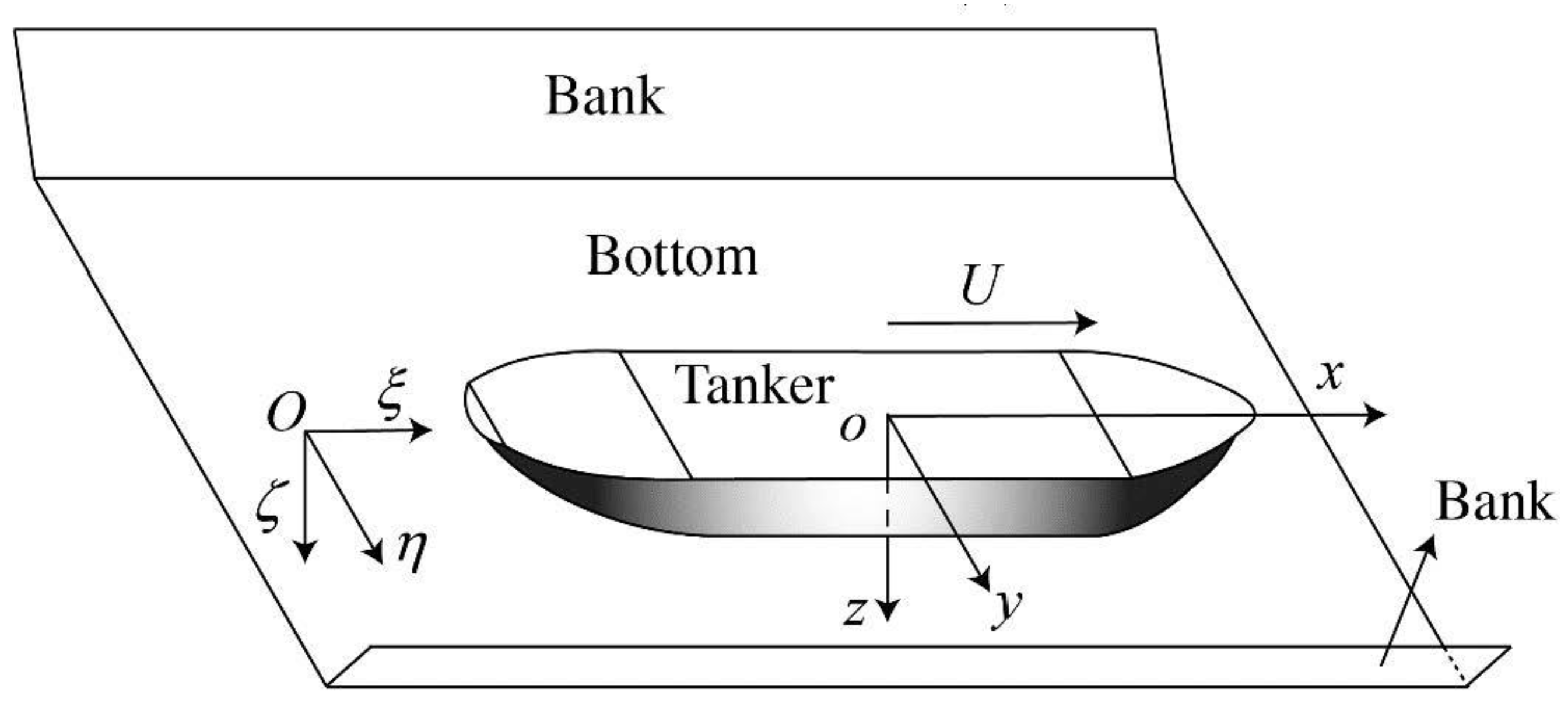
2.1. Coordinate Systems Definition and Transformation

The problem of concern is a ship moving along a channel at a constant speed U, as shown in Figure 1, where two different coordinate systems are used to describe the ship position and interaction forces. The earth-fixed coordinate $O\xi \eta \zeta$ is defined with the horizontal plane $\xi O\eta$ laid on the still free surface and the $\zeta$ axis pointing downward. A body-fixed coordinate $oxyz$ is defined with the origin o being the Center of Flotation (CoF); the x axis pointing the bow, positive forward; the y axis directed starboard; and the z axis downwards. The body-fixed frame $oxyz$ coincides with the earth-fixed at the outset, and moves with the captive model but free to sink and trim. The coordinates of origin o in the earth-fixed frame represent the advance ${\xi }_o$, the transfer ${\eta }_o$, and the sinkage ${\zeta }_o$, respectively. The angle between the x-axis and the $\xi O\eta$ plane is the trim (pitch) angle $\theta$. The coordinate transformation related the coordinates in the body-fixed frame to those in the earth-fixed frame and is given by:

$$\left\{G\left(P\right)\right\}=\left\{\begin{array}{c}Ut\\ 0\\ {\zeta }_o\end{array}\right\}+\left[\begin{array}{lll}\cos \theta & 0& \sin \theta \\ 0& 1& 0\\ -\sin \theta & 0& \cos \theta \end{array}\right]\left\{R\left(P\right)\right\},$$

(1)

where $G\left(P\right)$ is the global coordinates of point $P$, and $R\left(P\right)$ is the local coordinates of $P$.

2.2. Underlying Theory

Under the assumption that all interaction effects are caused by inertial hydrodynamic loads, the flow can be completely described with the total velocity potential $\Phi$ satisfying the Laplace equation in all fluid domain:

$${\nabla }^2\Phi =0.$$

(2)

The total velocity potential $\Phi \left(\xi ,\eta ,\zeta ,t\right)$ can be decomposed as:

$$\Phi =V_{\xi cur}\xi +V_{\eta cur}\eta +\varphi ,$$

(3)

where $V_{\xi cur}\xi +V_{\eta cur}\eta$ presents the steady velocity potential of the uniform horizontal current described by the velocity vector $V_{cur}$ or by its components $V_{\xi cur}$ and $V_{\eta cur}$, and $\varphi \left(\xi ,\eta ,\zeta ,t\right)$ is the disturbance potential. The non-penetration boundary condition is satisfied on the wetted surface of the ship hull $S_{hull}$:

$$\frac{\partial \varphi }{\partial n}=V_r\cdot n\mathrm{on}{S}_{hull},$$

(4)

the boundary condition on the bottom $S_{bottom}$ and bank $S_{bank}$ is:

$$\frac{\partial \varphi }{\partial n}=0\mathrm{on}{S}_{bottom}\mathrm{and}{S}_{bank},$$

(5)

where $n$ is the unit outward normal vector on the surface and the relative local velocity $V_r$ is:

$$V_r=V-V_{cur},$$

(6)

where $V$ is the local velocity at a point on the hull surface. Under the assumption of low Froude number, the double-body model is used to approximate the boundary condition on the free surface:

$$\frac{\partial \varphi }{\partial \zeta }=0\mathrm{on}\zeta =0.$$

(7)

A common method of solving the Neumann boundary value problem defined by Equation (2), (4), (5) and (7) is based on distribution of a single layer of sources on the wetted surface of the ship, bottom and also the bank. Then, the induced velocity potential at the field point $P\left({\xi }_P,{\eta }_P,{\zeta }_P\right)$ is:

$$\varphi \left(P\right)={\displaystyle \underset{S}{\iint }\sigma \left(Q\right)G\left(P,Q\right)}\mathrm{d}S\left(Q\right),$$

(8)

where S is the boundary $S=S_{hull}+S_{bottom}+S_{bank}$, $Q\left({\xi }_Q,{\eta }_Q,{\zeta }_Q\right)$ is the source point on the boundary surface, and $\sigma \left(Q\right)$ is the source strength. Substituting Equation (4) and (5) into Equation (8) yields a Fredholm integral equation of second kind for the source density:

$$2\pi \sigma \left(P\right)+{\displaystyle \underset{S}{\iint }\sigma \left(Q\right)\frac{\partial G\left(P,Q\right)}{\partial n\left(P\right)}}\mathrm{d}S\left(Q\right)=f\left(P\right),$$

(9)

where the right-hand side of Equation (9) takes different values depending on the location of the point P: is $f\left(P\right)=V_r\cdot n\left(P\right)$ if the point P is on the ship hull, and is $f\left(P\right)=0$ on the seabed. In the double-body model the Green function,

$$G\left({\xi }_P,{\eta }_P,{\zeta }_P,{\xi }_Q,{\eta }_Q,{\zeta }_Q\right)=\frac{1}{r}+\frac{1}{\overline{r}}$$

(10)

is used, where $r=\sqrt{{\left({\xi }_P-{\xi }_Q\right)}^2+{\left({\eta }_P-{\eta }_Q\right)}^2+{\left({\zeta }_P-{\zeta }_Q\right)}^2}$ and $\overline{r}=\sqrt{{\left({\xi }_P-{\xi }_Q\right)}^2+{\left({\eta }_P-{\eta }_Q\right)}^2+{\left({\zeta }_P+{\zeta }_Q\right)}^2}$.

The body surface is approximated with quadrilateral elements, and over each of them, the source strength $\sigma$ is assumed constant. Equation (9) can be approximated by a set of linear algebraic equations:

$$A_{ij}{\sigma }_j=B_i,$$

(11)

which can be solved using the Gauss-Seidel or Gauss-Jordan method. Once the source strengths are obtained, the disturbance potential $\varphi$ and induced velocity $V_I$ on the element can be calculated by:

$$V_I\left(P\right)={\displaystyle \sum _j^n{\sigma }_j{\displaystyle \underset{\Delta S_i}{\iint }{\nabla }_P}}G\left(P,Q\right)\mathrm{d}S\left(Q\right),$$

(12)

$$\varphi \left(P\right)={\displaystyle \sum _j^n{\sigma }_j{\displaystyle \underset{\Delta S_i}{\iint }G\left(P,Q\right)\mathrm{d}S\left(Q\right)}}.$$

(13)

The pressure distribution is then calculated using the unsteady Bernoulli equation [31]:

$$p=\rho \left[-\frac{\partial \varphi }{\partial t}+\frac{1}{2}\left(V_r^2-V_p^2\right)\right],$$

(14)

where $\rho$ is the density of fluid, and the “pressure” velocity is:

$$V_P=V_I-V_r.$$

(15)

The total forces and moments are obtained by integrating the pressure over the ship hull:

$$F=X{e}_x+Y{e}_y+Z{e}_z=-{\displaystyle \underset{S_{hull}}{\iint }p}n\mathrm{d}S,$$

(16)

$$M=K{e}_x+M{e}_y+N{e}_z=-{\displaystyle \underset{S_{hull}}{\iint }p\left(r\times n\right)}\mathrm{d}S.$$

(17)

In general, to obtain the net interaction forces, it is necessary to estimate and subtract the proper hydrodynamic inertial forces appearing when the ship’s motion is different from a uniform rectilinear. This can be done using the approach described in [13], but in the cases analyzed within the scope of the present paper, this was not required.

2.3. Determination of Sinkage and Trim

Hydrodynamic forces and moments acting on the ship in the vertical planes will alter its attitude which is called the squat phenomenon. In this study, the resulting sinkage ${\zeta }_o$ and trim angle $\theta$ can be estimated using an iterative procedure with five steps, as shown in Figure 2:

(1)

Initialize the parameters, including advance $\xi$, transfer $\eta$, velocity U, iteration number n, flotation, etc.

(2)

Obtain the vertical force Z and pitch moment M based on the numerical solution mentioned in Section 2.2.

(3)

Calculate the variation of draft $\delta {\zeta }_0$ and trim $\delta \theta$, and then update the flotation.

(4)

If both $\delta {\zeta }_0$ and $\delta \theta <{\epsilon }_2$ hold, then go to Step 5; if not, n = n + 1, and turn to Step 2.

(5)

The sinkage and trim are finally determined.

where ${\epsilon }_1$ and ${\epsilon }_2$ are the convergence criteria for sinkage and trim, respectively. At each iterative step, the variation of sinkage $\delta {\zeta }_0$ and trim $\delta \tau$ are determined with the following formulas resulting from the standard linear ship hydrostatics:

$$\begin{array}{l}\delta {\zeta }_o=\frac{1}{\rho A_{WL}}\cdot \frac{\nabla G{M}_{L}Z-A_{WL}{x}_{F}M}{\nabla G{M}_L-A_{WL}{x}_F^2},\\ \delta \theta =\frac{1}{\rho }\cdot \frac{M-Z{x}_F}{\nabla G{M}_L-A_{WL}{x}_F^2},\end{array}$$

(18)

where $\nabla$ is the ship displacement, $G{M}_L$ is the longitudinal metacentric height, $A_{WL}$ is the waterplane area and $x_F$ is the abscissa of the flotation center. When the ship is sailing near a bank, dynamic heel may also occur but this effect is ignored in the present study.

As the submerged part of the ship’s hull is altered due to the sinkage and trim, this may affect the estimated interaction loads, and to account for that, repaneling must be performed. In the present study, this was performed with the panel trimming technique described in detail in [30].

3. Ship Model, Canals and Test Conditions

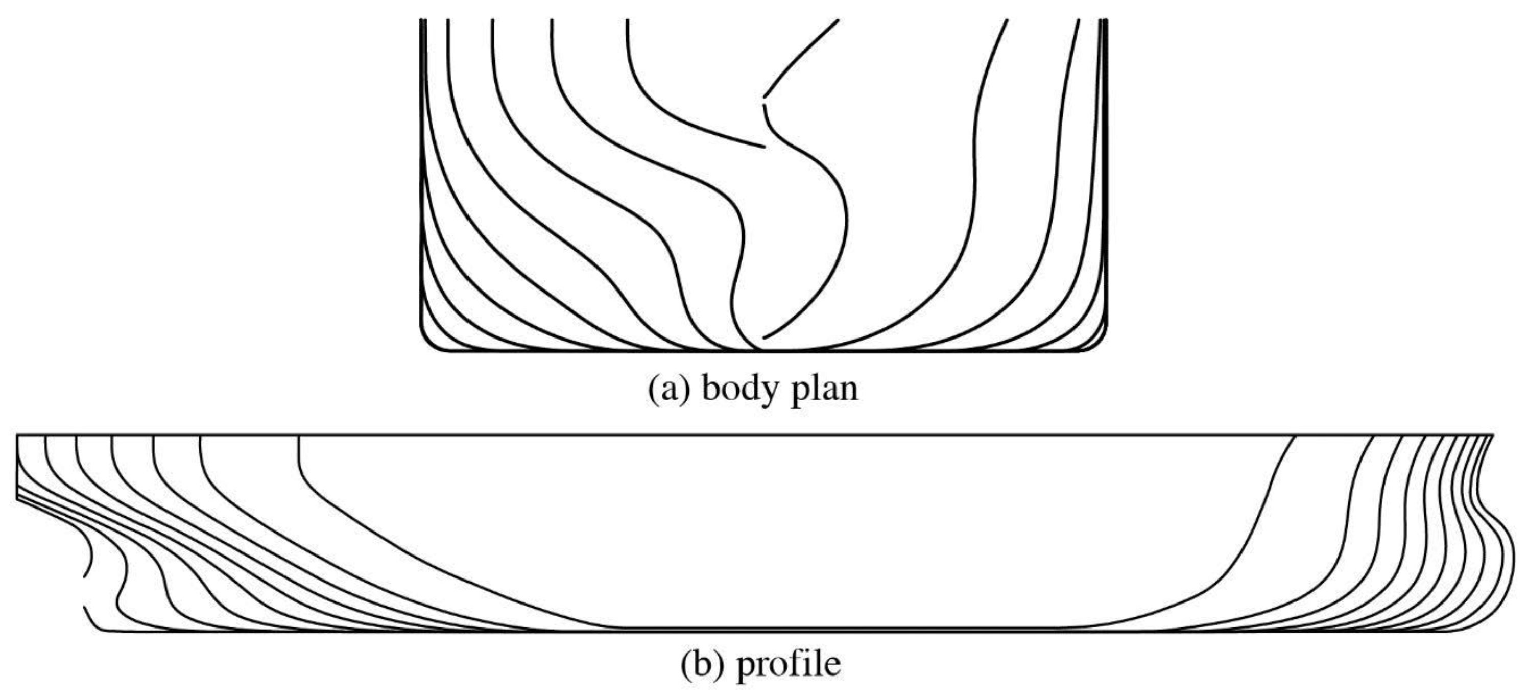
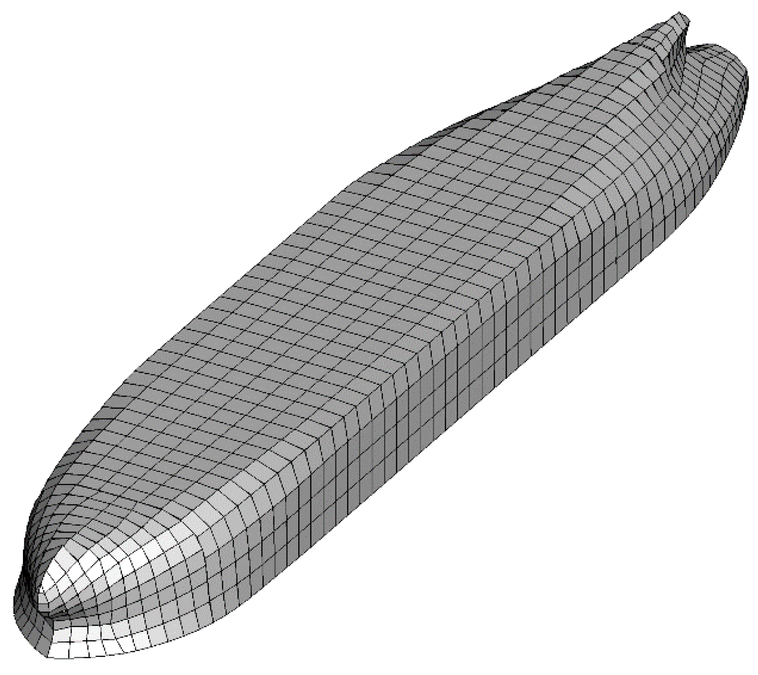
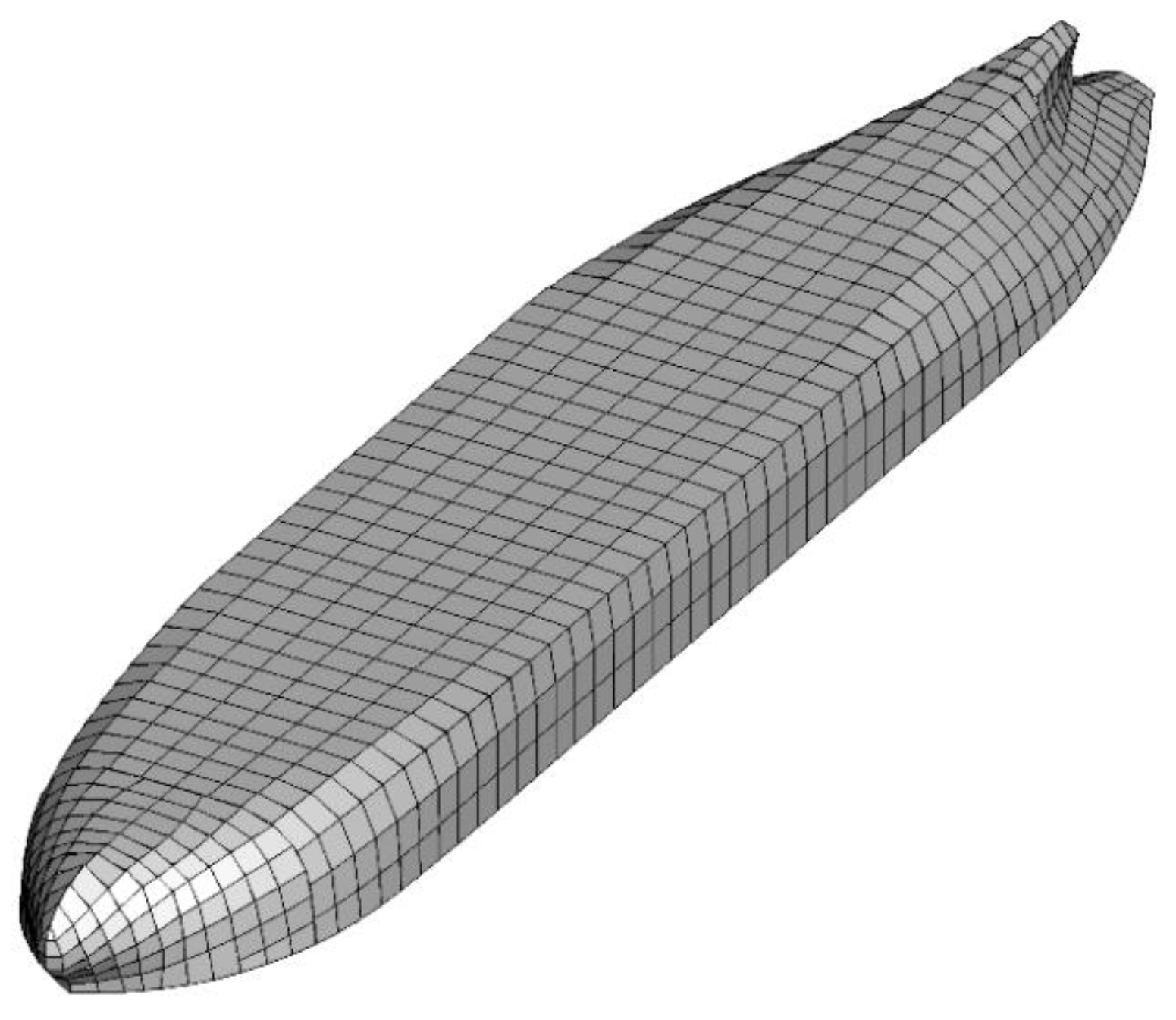
3.1. Ship Model

The KRISO Very Large Crude Carrier (KVLCC2) is used to investigate the ship-bank effect. For this ship form, Flanders Hydraulics Research (FHR) has conducted a series of model tests for various parameters, such as water depth, ship-bank distance, and bank profile. The experimental values, including surge force $X$, sway force $Y$, heeling moment $K$, yaw moment $N$, sinkage ${\zeta }_0$ and trim $\theta$, can be found in Zou and Larsson [6] and Van Hoydonck et al. [8]. These data are widely used for validation and verification [6,8,18].

A 1/75 scale model of KVLCC2 is used in the simulations. The principal particulars of KVLCC2 are shown in

Table 1. Principle particulars of the KRISO Very Large Crude Carrier (KVLCC2) in full-scale and model scale.

Parameters	Full Scale	Model Scale
Length ($L_{PP}$) (m)	320.0	4.2667
Breath ($B$) (m)	58.0	0.7733
Draft at midship ($T$) (m)	20.8	0.2776
Longitudinal CoG ($x_G$) (m)	10.87	0.1449
Vertical CoG ($z_G$) (m)	20.8	0.2776
Longitudinal CoF ($x_w$) (m)	−2.67	−0.0356
Waterplane area ($A_w$) (m2)	16,706.25	2.9700
Displacement ($\nabla$) (m3)	312,622	0.7410
Longitudinal metacentric height ($G{M}_L$) (m)	398.55	5.3140
Block coefficient ($C_B$)	0.8098	0.8098

where CoG is the center of the gravity, and the body plan and profile of KVLCC2 in Figure 3. As shown in Figure 4, the entire hull surface is discretized into 1036 panels, 190 for the bow ($x>1.706\mathrm{m}$), 704 for the parallel body ($-1.706\mathrm{m}\le x\le 1.706\mathrm{m}$), and 142 for the stern ($x<-1.706 \mathrm{m}$). The panels used for simulation are generated from the mesh for the entire hull surface and vary with the predicted sinkage and trim. The discretization of the portion below the instantaneous waterline at the initial instant (0.2776 m draft, 0° trim) is shown in Figure 5, where 874 panels are used to approximate the wetted surface, which has been proven sufficient for ship hydrodynamic interaction simulations [13].

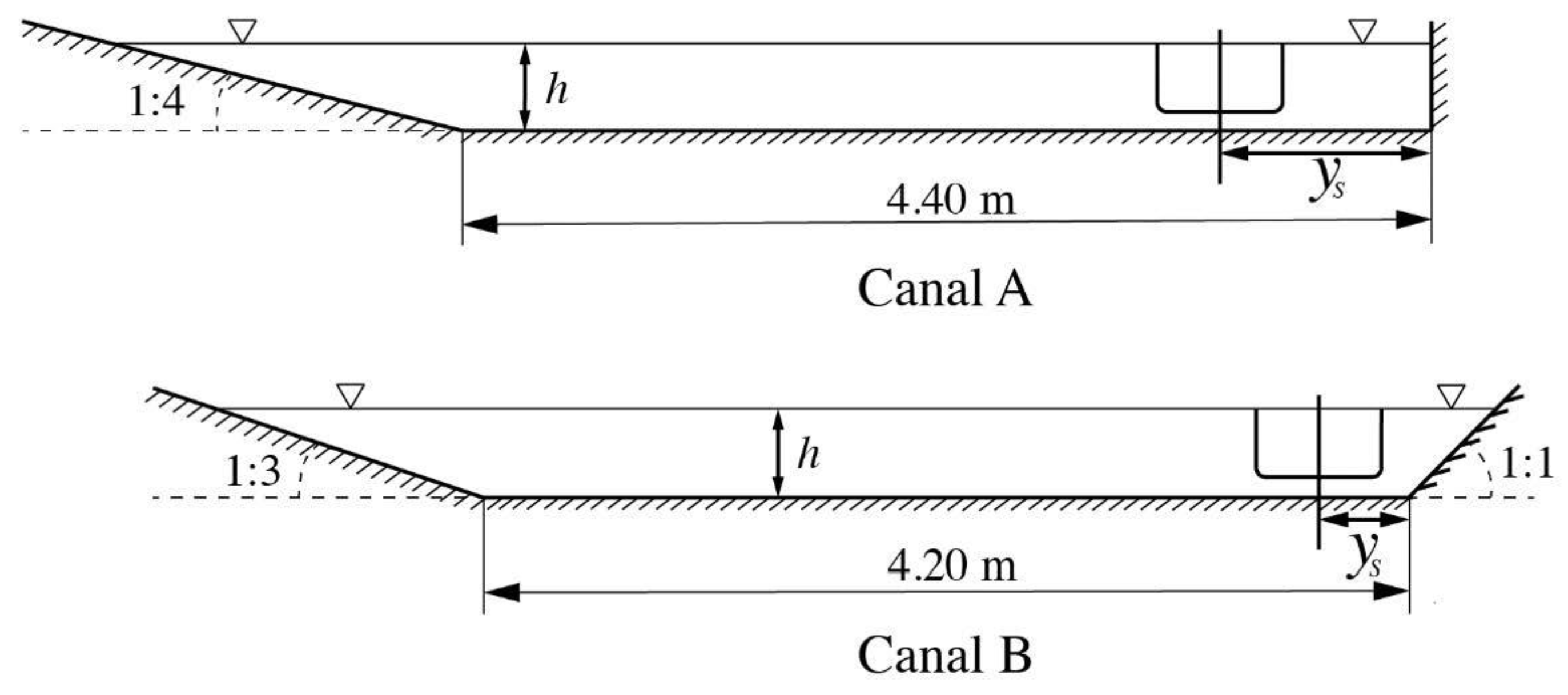
3.2. The Canals

Two different canal profiles were investigated: Canal A and Canal B. The former has a vertical wall on the right-hand side and a 1:4 slope bank is on the other. The latter has two sloped banks, one of which has a slope of 1:1, and the other a slope of 1:3, as shown in Figure 6. The lateral distance between the center-plane of the ship and the bottom of the bank is denoted as y_s.

In the application of the paneled moving patch method, sources are distributed; in addition to the wetted hull surface, also over some finite domain (patch) of the bottom beneath the moving hull, and this patch moves with the ship so as to take into account the bottom and bank effect in the simulation. Both the panel size and the dimensions of the patch directly affect the computational efficiency. Larger patches and finer grids will produce better accuracy, while the computational cost also increases. For this reason, a convergence analysis is performed to determine the size of patch and panel for the canal. For the patch size, a set of calculations with various patch length is carried out where the length of the patch on the canal bed/bank ranges from 6 m to 22 m, and square-shaped panels with a side length of 0.2 m are used. The KVLCC2 model was moving along the bank in Canal A at a constant speed of 0.356 m/s, with the depth-to-draft ratio $h/T=1.35$, and the ship-bank distance $y_s=0.5175 \mathrm{m}$. The numerical results with varying patch length are obtained and plotted in Figure 7. As can be seen from all the numerical results for the forces, sinkage and trim converge as the patch length increases.

It can be observed from Figure 7 that a larger patch length can improve the accuracy while the computational cost is also higher. Therefore, it is unwise to use extra-large patch sizes when the computational efficiency is also a concern. According to the convergence analysis, the patch length of 18 m is chosen for the simulations in this study, i.e., 4.22 times the model length of KVLCC2.

A similar convergence analysis is carried out to determine the panel size for the canal with the panel size ranging from 0.15 m to 1.0 m, and the patch length takes 18 m according to the convergence pattern in Figure 7. The test case used in the convergence analysis of the patch length is used, and the numerical results calculated with different panel sizes are shown in Figure 8. It is found that the results are well behaved when the panel size is smaller than 0.25 m. Since there are cases with shallower water depths and smaller ship-bank distances in the study, the panel size for the canal takes 0.2 m so as to obtain reliable results. The discretization of Canal A is shown in Figure 9, where the maximum panel size is 0.2 m.

3.3. Test Conditions

In this study, 12 cases with different water depths, ship-bank distances and bank profiles were investigated: 8 cases for Canal A, and 4 cases for Canal B. The configurations of these cases are listed in

Table 2. Test conditions matrix for Canal A.

h (h/T)	Frh	ys
		0.5175 m	0.5866 m	0.9731 m	1.3594 m
0.4160 m (1.50)	0.1763		Case 7	Case 4
0.3744 m (1.35)	0.1859	Case 1	Case 2	Case 3	Case 6
0.3051 m (1.10)	0.2059		Case 8	Case 5

and

Table 3. Test conditions matrix for Canal B.

h (h/T)	Frh	ys
		0.3170 m	0.3872 m	0.7735 m	1.1613 m
0.3744 m (1.35)	0.1859	Case 9	Case 10	Case 11	Case 12

. In all the cases, KVLCC2 was advancing at the same speed of U = 0.356 m/s which corresponds to the depth-based Froude numbers shown in Table 2. No current was produced in the tank, thus, the velocity of the current in Equation (3) is zero.

4. Comparison and Analysis

In addition to the validation of the present method against experiment, all the cases are simulated twice: one with fixed sinkage and trim, while the other with free sinkage and trim. The numerical results of these simulations are compared with the experiment, Rankine source and RANSE-based simulations. The influence of sinkage and trim on the estimated interaction forces is also analyzed.

The experimental results of cases 1–5 can be found in Van Hoydonck et al. [8], and those of cases 1–3 and 6–12 are in Zou and Larsson [6]. However, those presented in the latter are processed in the manner as follows:

$$\begin{array}{l}\overline{X}=X^{\prime }/Y_{\max }^{\prime },\overline{Y}=Y^{\prime }/Y_{\max }^{\prime },\\ \overline{K}=K^{\prime }/K_{\max }^{\prime },\overline{N}=N^{\prime }/K_{\max }^{\prime },\\ {\overline{\zeta }}_0={\zeta }_o/{\zeta }_{o\max },\overline{\theta }=\theta /{\theta }_{\max },\end{array}$$

(19)

where X′, Y′, K′, N′, are the nondimensionalized values for surge force, sway force, heeling moment and yaw moment:

$$\begin{array}{l}{X}^{\prime }=\frac{X}{\frac{1}{2}\rho U^2{L}_{pp}T},Y^{\prime }=\frac{Y}{\frac{1}{2}\rho U^2{L}_{pp}T},\\ K^{\prime }=\frac{K}{\frac{1}{2}\rho U^2{L}_{pp}{T}^2},N^{\prime }=\frac{N}{\frac{1}{2}\rho U^2{L}_{PP}^{2}T}.\end{array}$$

(20)

The subscript ‘max’ in Equation (19) denotes the maximum measures appeared in all the cases investigated in the study, which, however, are not explicitly given in the publication [6]; and the bar on top of a symbols stands for relative values.

Since the same cases, i.e., cases 1–3, are presented in both Van Hoydonck et al. [8] and Zou and Larsson [6], the maximum measures undisclosed in Zou and Larsson [6] can be calculated from the absolute experimental values provided in Van Hoydonck et al. [8], and the absolute values of the cases 6–12 can be adopted. For example, for the sway force, the non-dimensional results $Y_i^{\prime }(i=1,2,3)$ for the cases 1–3 can be calculated from the absolute values $Y_i(i=1,2,3)$ given in Van Hoydonck et al. [8], and then $Y_{\max }^{\prime }$ in Equation (19) can be calculated $Y_{\max }^{\prime }=Y_i^{\prime }/\overline{Y_i}$ as $\overline{Y_i}(i=1,2,3)$ is given in Zou and Larsson [6]. This $Y_{\max }^{\prime }$ also applied to the processing of the results of cases 6–12, thus, $Y_i^{\prime }={\overline{Y}}_i\times Y_{\max }^{\prime }(i=6,\dots ,12)$, and finally, the absolute values $Y_i(i=6,\dots ,12)$ of the cases 6–12 can be obtained using Equation (20).

Besides the test data, comparisons with the RANSE-based method [6,8] and the Rankine source method [18] have also been carried out whenever possible.

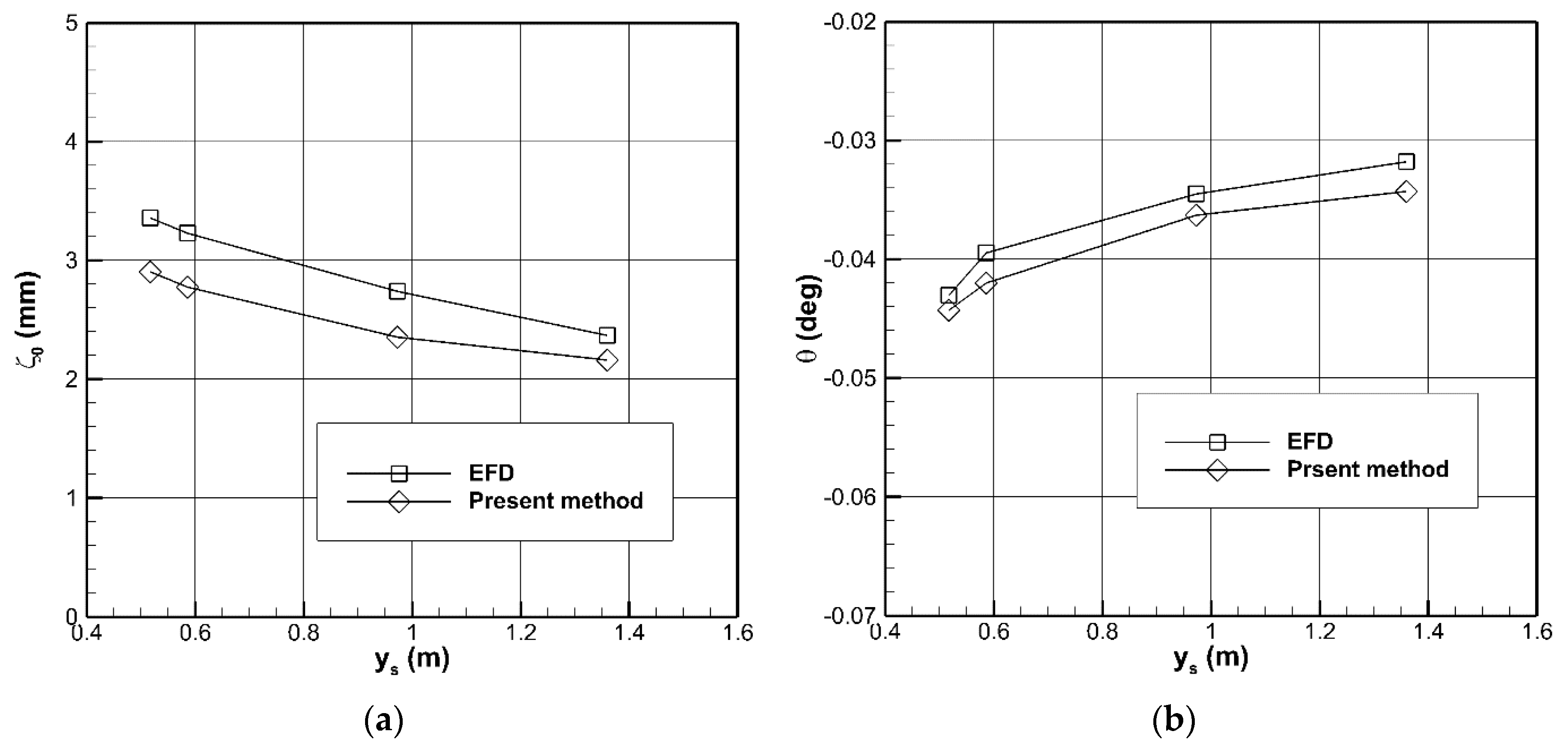
4.1. Sinkage and Trim in Canal A

The numerical results obtained with the present method for the sinkage and trim in Canal A are plotted in Figure 10, Figure 11 and Figure 12, together with the experimental ones as those obtained with the RANSE code: EFD in the legends corresponds to the experimental results, CFD—to the RANSE simulations, and Rankine—to the results obtained by the free-surface Rankine source method.

As shown in Figure 10, the sinkage and trim increase with reduction of the ship-bank distance, and a significant bank influence on the squat is observed. The estimated sinkage and trim with various ratios of h/T at two different ship-bank distances are plotted in Figure 11 and Figure 12. It can also be seen that the sinkage and trim increase as the water depth reduces.

Regarding the sinkage, the tendencies are well captured with the present numerical method. It can be also observed from the figures that, the present method, in general, somewhat underestimates the sinkage, and the discrepancy becomes larger as the ship gets closer to the bank and the bottom, especially, for the extreme condition of h/T = 1.1. The RANSE-based method is more accurate, which suggests that the viscous effect is non-negligible in this case, as shown in Figure 11a. On the other hand, the free surface effect seems to be insignificant as long as it was not considered in the viscous flow simulations [18].

The stern down trim due to the bank effect is also captured by the present method with fair accuracy, even if the viscosity effect and free surface effect are both neglected. As shown in Figure 11b, the error in the estimate for the trim is still acceptable for the most extreme condition, i.e., h/T = 1.1 and y_s = 0.5866 m. Comparison of the present method with the RANSE-based simulation of the case of h/T = 1.1 shows that RANSE-based simulation accounting for viscosity is not more accurate because the estimates for the trim by both methods are almost the same.

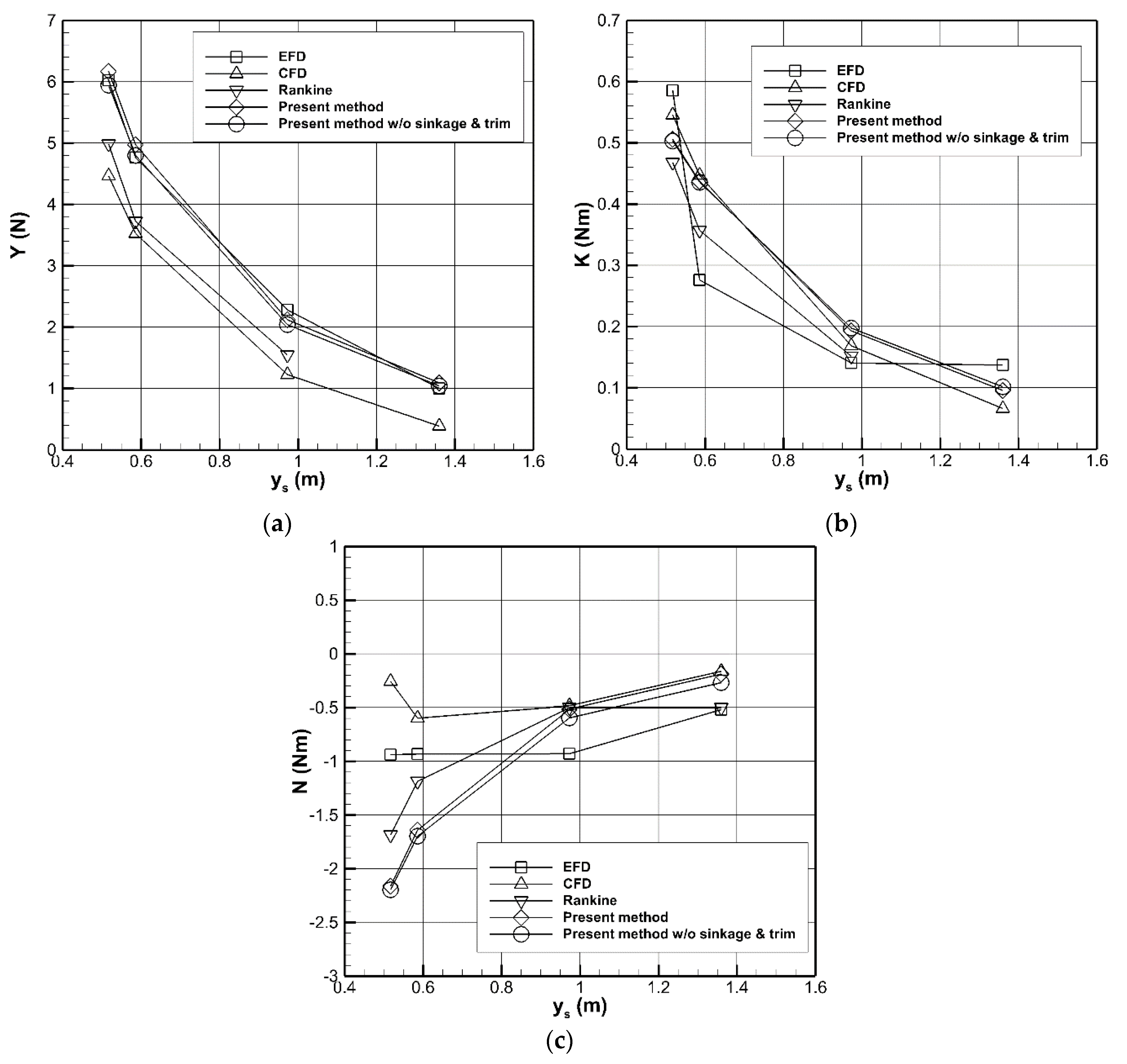
4.2. Hydrodynamic Forces and Moments in Canal A

The estimated interaction forces and moments of KVLCC2 moving in parallel to the vertical wall are plotted in Figure 13 as a function of ship-bank distance y_s, where the results of model test, viscous flow simulation, and Rankine source method are also given for the purpose of comparison. The numerical results with/without accounting for sinkage and trim are both presented in this section as to analyze their contribution to the hydrodynamic interaction forces.

As shown in Figure 13a,b, the exponential growth of the sway force and the heeling moment as the ship approaches the bank, indicates the important influence of the bank on the interaction forces. It is demonstrated that, from the comparison with the experimental results, the method neglecting the viscosity and the free surface effect can also estimate the ship-bank interaction forces with satisfying accuracy. Remarkably, for sway force, the present method turns out to be the most accurate. The reason that the present method in some cases performs better than the RANSE-based method is that the neglecting of the free surface effect will introduce errors, so will neglecting the viscosity, however, it is in this case, these two types of different origins make opposite contributions and the global numerical results turn out to be closer to the experiment than neglecting either free surface effect or viscosity alone, i.e., the errors cancel each other. A similar error cancelation effect has also been reported in Ref. [24] where RANSE- based simulations of ship hydrodynamic interaction are performed with and without accounting for the viscosity and free surface effect. However, in neither case, such error cancellation effects shall be generalized.

The yaw moment in the extreme conditions, i.e., $y_s\le 0.5866\mathrm{m}<B=0.7733\mathrm{m}$, is overestimated by the present method. It can be seen in Figure 13c that the Rankine source-based method, in which the free surface effect is accounted for, performs somewhat better, but the pattern is similar to that shown by the present method, and the values are also far away from the experiment. The difference at $y_s\le 0.5866\mathrm{m}$ may be caused by the drop of the free surface drop at the side of bank, and the influence of free surface also plays a significant role on yaw moment at a relatively small ship-bank distance even in the intermediate water depth. The RANSE-based code also failed to produce a reasonable estimate in this case. For larger ship-bank distances y_s, the pattern of the yaw moment obtained by the present method is similar to the experiment, however, there is still a difference, as shown in Figure 13c. Interestingly, the present method shows a very good agreement with both RANSE-based simulation and the Rankine source-based method. It seems that considering the free surface effect or the viscosity alone in the numerical methods does not help much with producing more accurate results in this case.

The hydrodynamic interaction forces and moments at y_s = 0.5866 m and y_s = 0.9731 m are presented in Figure 14 and Figure 15 as function of the relative water depth. As shown in Figure 14a and Figure 15a, the present method, in general, overestimates the sway force for the case of the extreme shallow water (h/T = 1.1). Actually, the effect of the free surface is significant in very confined waters [8], the level difference between both sides of the hull is relatively large, and the double-body model is not suitable in these cases—in which cases, the Rankine source method performs better. Accounting for the sinkage and trim helps with the accuracy of the calculation for both ship-bank distances, while the improvement is small which could be expected at small changes of attitude. A comparison of Figure 14a and Figure 15a shows that the present method is less accurate as the ship-bank distance decreases from y_s = 0.9731 m to y_s = 0.5866 m, but still the relative error is smaller than 15% (except for the extreme shallow water case). This suggests that the present method is fairly accurate in estimating the sway force for moderate shallowness.

For the heeling moment, the numerical results obtained by the present method have a pattern similar to the experiment. For the case of y_s = 0.5866 m, the heeling moment is slightly underestimated by the present method at h/T = 1.1. For larger ratios of h/T, all the numerical approaches produce almost the same results that are overestimated to some extent, with a relatively larger error at h/T = 1.35 and a smaller error at h/T = 1.50, as shown in Figure 14b. At y_s = 0.9731 m, the pattern is correctly captured by the present method, with a slight underestimation for the case h/T = 1.1 and some overestimation for other water depths. In comparison, the RANSE-based method fails to estimate the force at h/T = 1.1, but looks very accurate for other water depths. Based on the comparisons for the heeling moment as shown in the Figure 13b, Figure 14b and Figure 15b, it can be stated that the present method is able to estimate the heeling moment with a fair accuracy.

For y_s = 0.5866 m and h/T = 1.1, the yaw moment is significantly underestimated by the present method. In this case, only the RANSE-based method was able to give reasonable estimates. For other water depths at the same ship-bank distance, however, the present method performed even better than the RANSE-based method in terms of accuracy. A possible reason for the better accuracy of the present method than the RANSE-based method in neglecting the free surface effect is that there might be a cancellation effect between the errors resulted from neglecting the free surface effect and those from neglecting the viscosity. For y_s = 0.9731 m, the present method produces almost the same results as the Rankine source-based method, and both of them failed to estimate the yaw moment for the extreme shallow water case of h/T = 1.1. For other water depths, the present method and the Rankine source-based method agree well with the experiment. Thus, as can be seen from the comparisons, the present method is also able to estimate the yaw moment except for the extreme shallow water case, which, however, should be avoided in navigation [32].

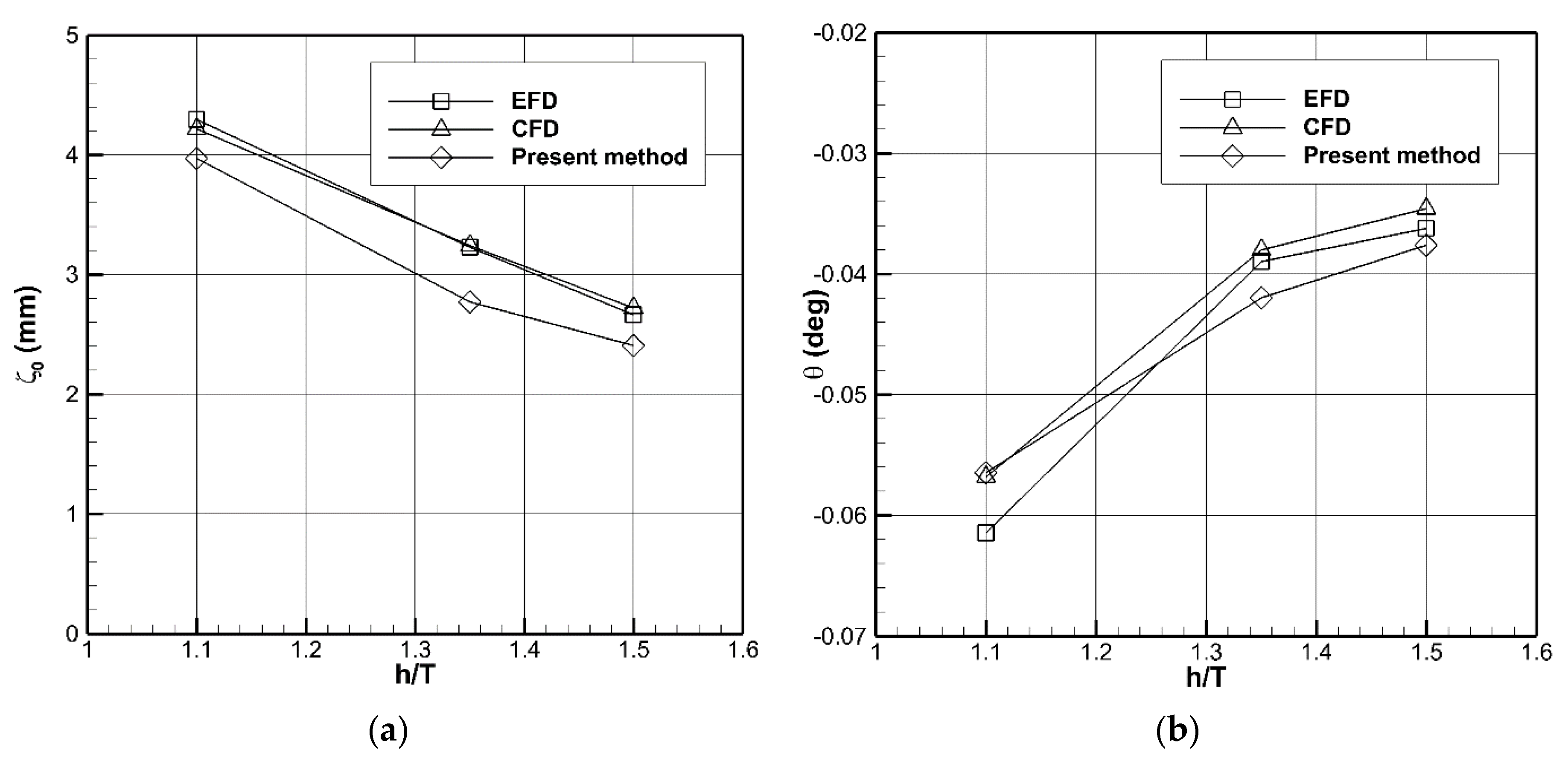
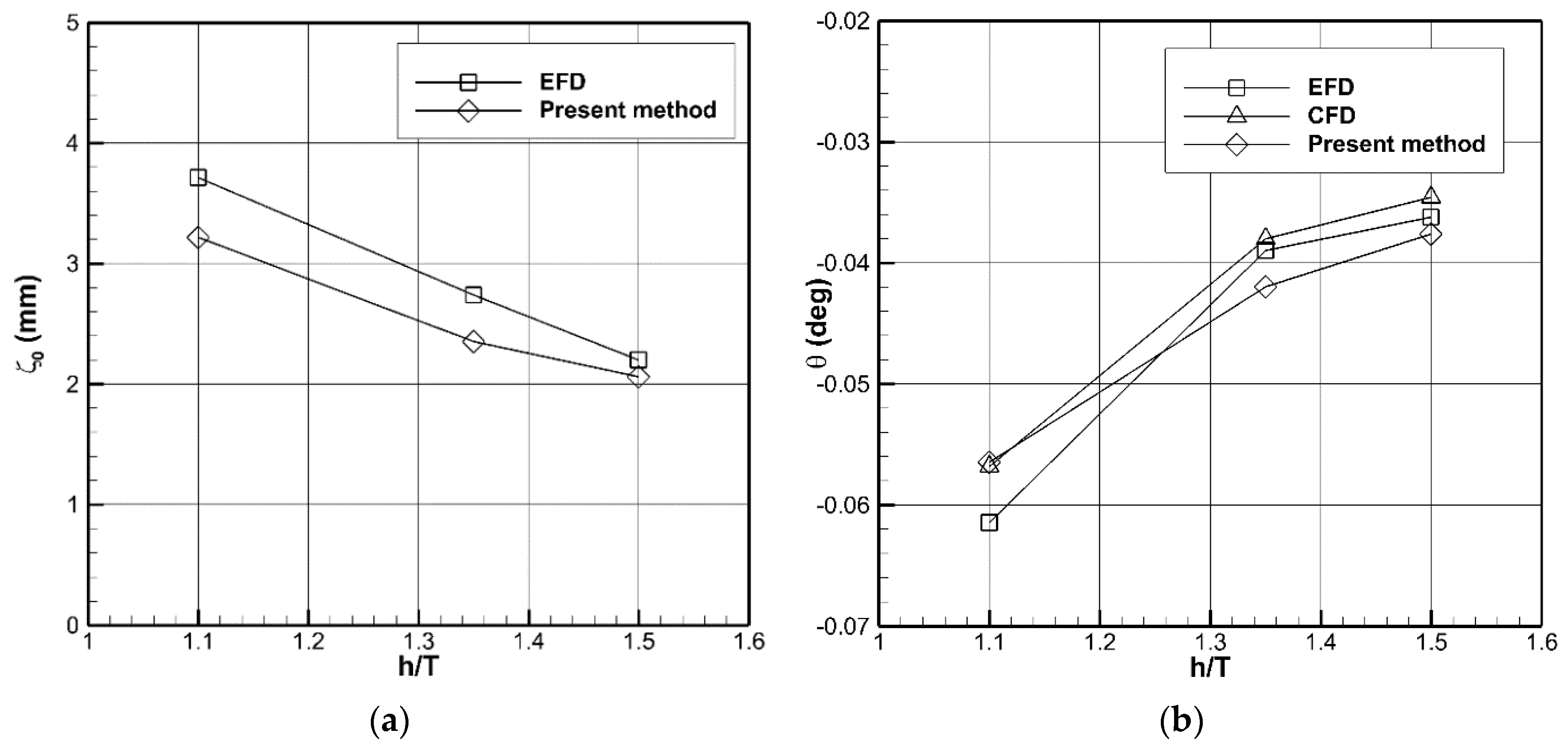
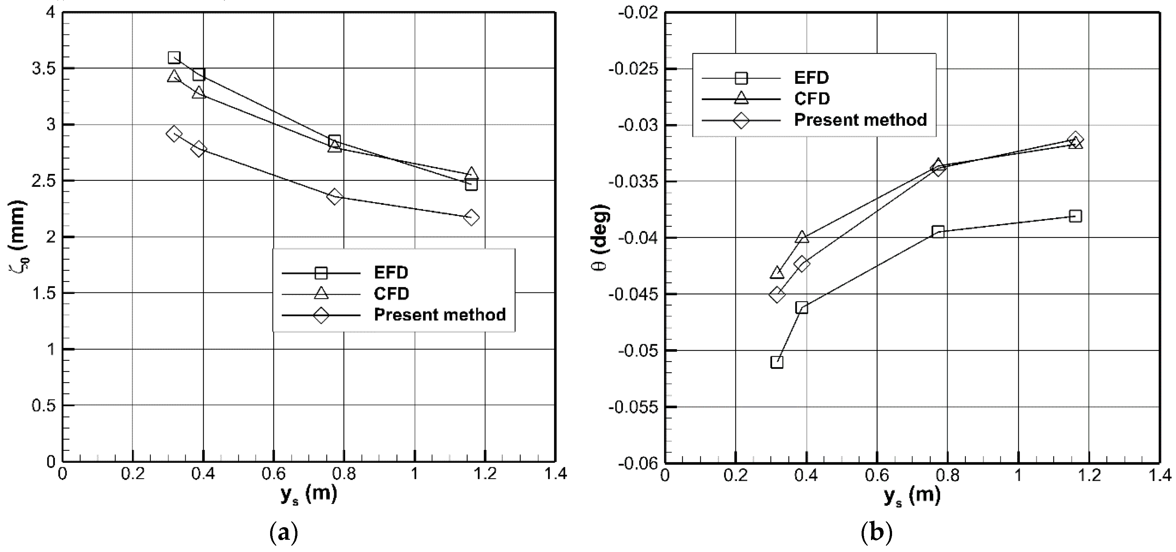
4.3. Sinkage and Trim in Canal B

In this section, a set of simulations of KVLCC2 moving along a sloped bank is carried out, and the results for the sinkage and trim with various lateral distances are plotted in Figure 16. It can be seen that the smaller is the ship-bank distance, the larger is the sinkage and trim.

For the sinkage, this trend is well captured by both the RANSE-based method and the present method. The former is very accurate, while the latter exhibits the error of 19% for the smallest bank distance, which reduces to 10% as the distance increases.

The superiority of the RANSE-based method is very limited in the calculation of the trim, as shown in Figure 16b, and, in fact, for the small ship-bank distances, the present methods even produce more accurate results. For all investigated ship-bank distances, the relative error of the present method remains within the range from 12% to 18%. The discrepancies likely result from neglecting the free surface viscosity effects.

In general, the present method is able to produce results for the sinkage and trim with acceptable accuracy.

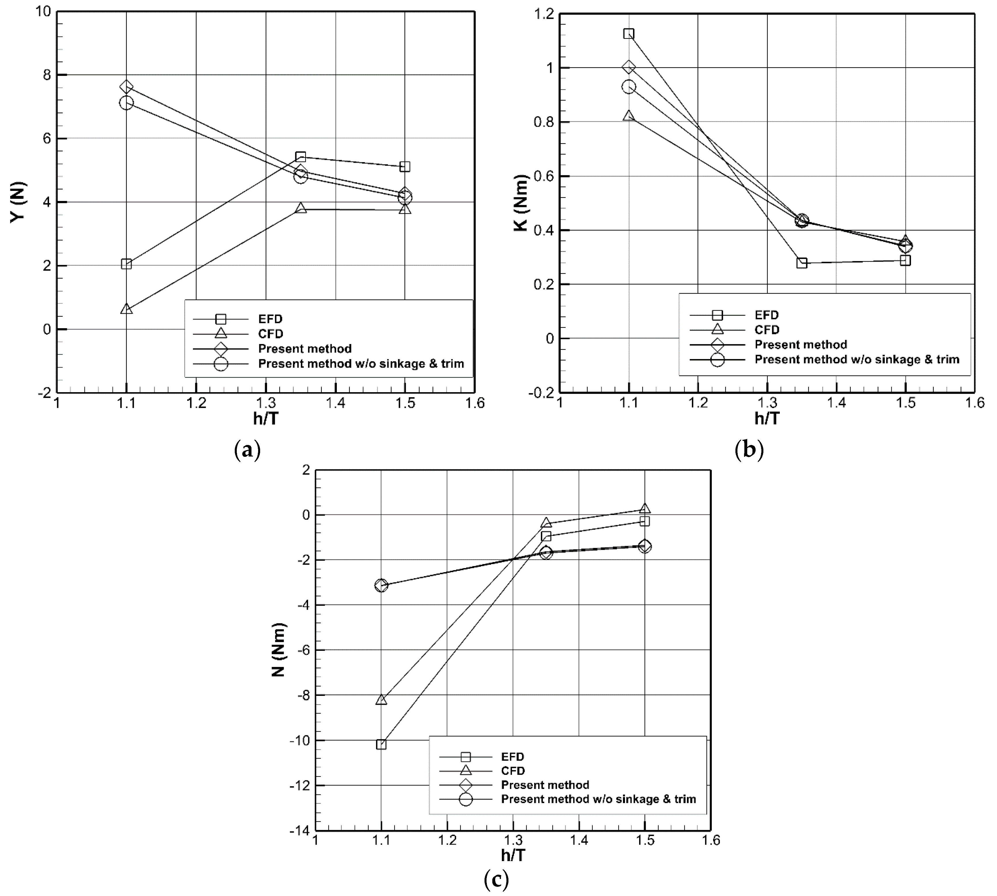
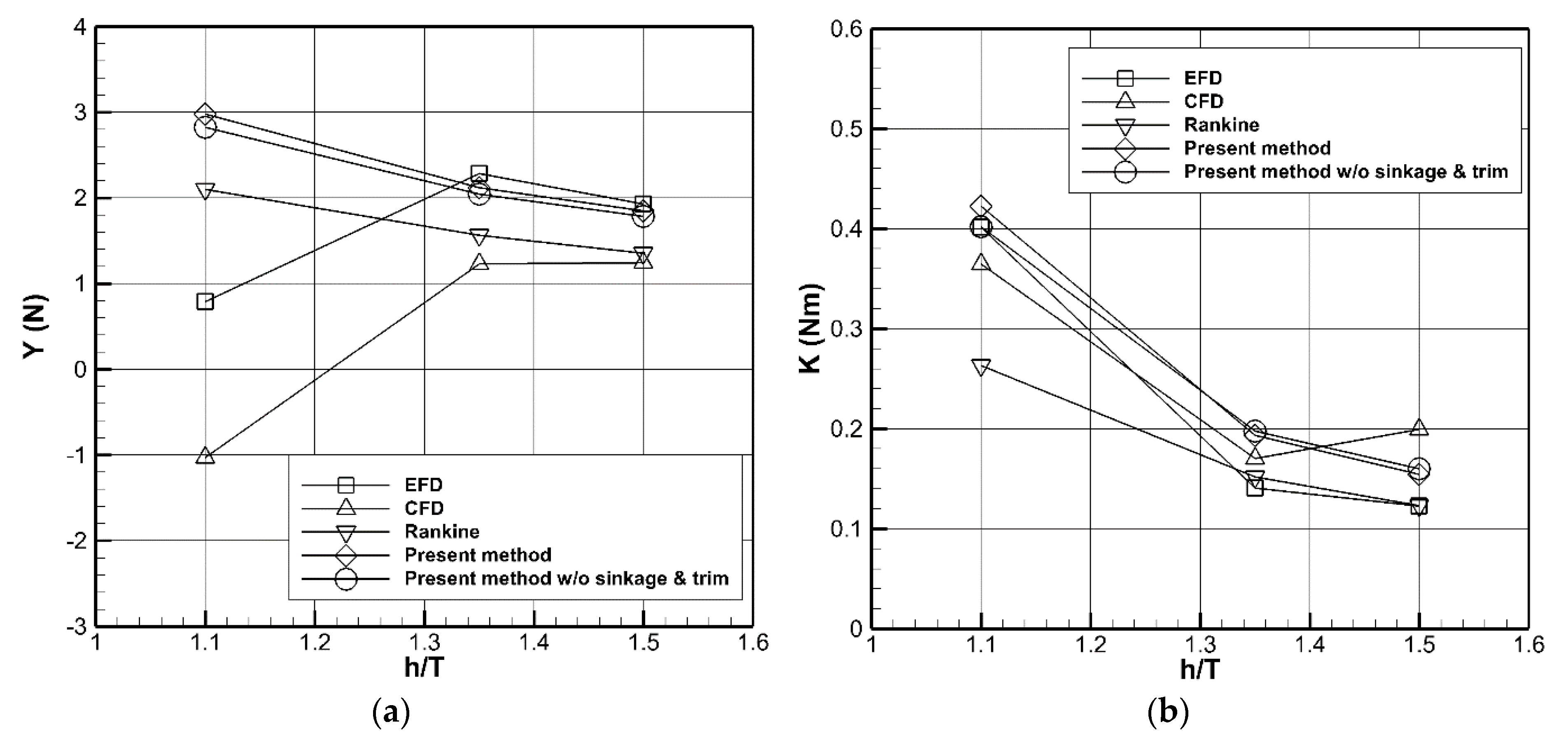
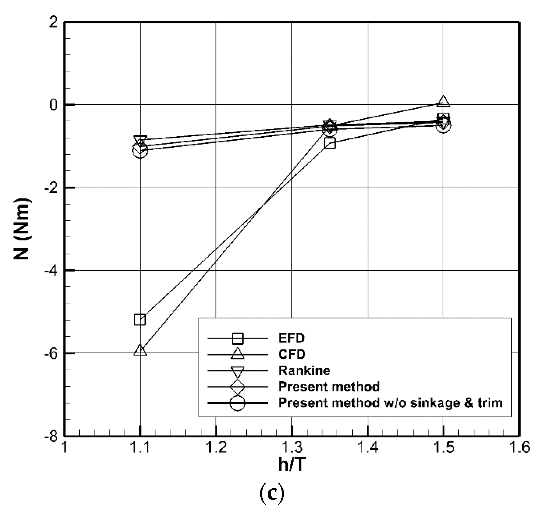
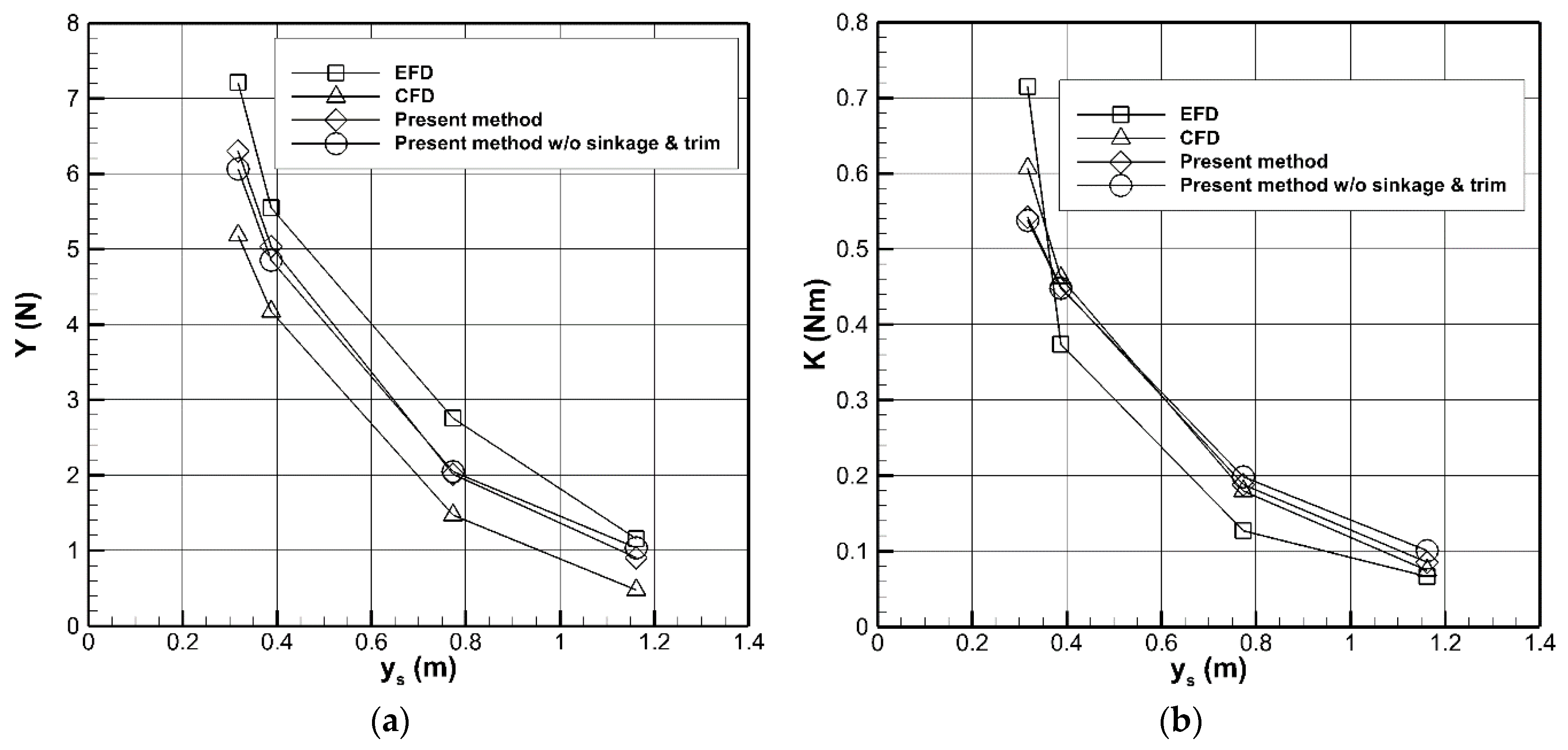
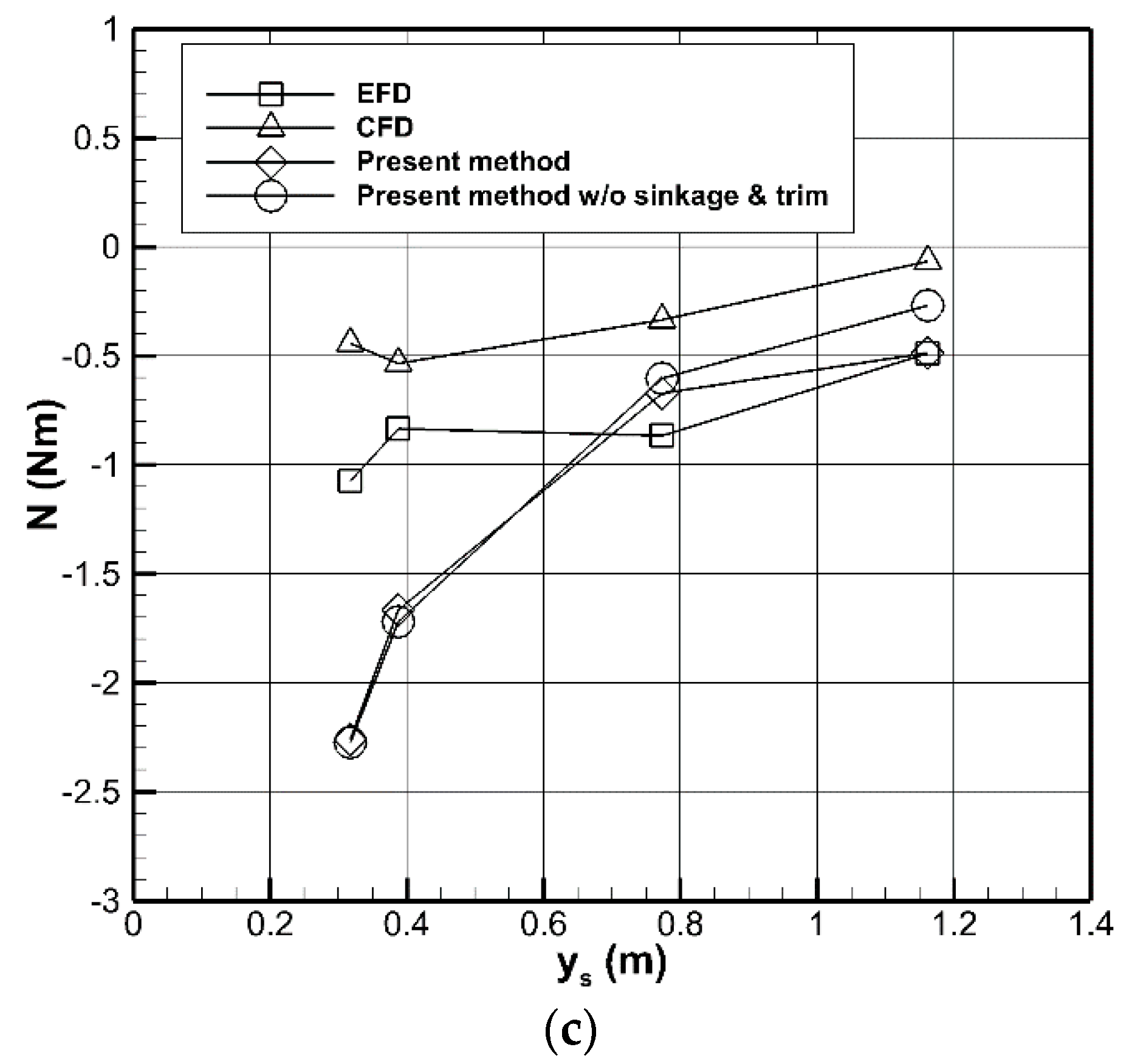
4.4. Hydrodynamic Forces and Moments in Canal B

The results for the interaction forces in Canal B obtained by the present method with and without accounting for sinkage and trim are plotted in Figure 17. Similarly to the case of the vertical bank wall, the forces increase as the ship-bank distance decreases. The sinkage is slightly underestimated but the accuracy is satisfactory. Another observation is that the RANSE-based method is again less accurate in this case, possibly because of the error cancellation effect mentioned above.

For the heeling moment at the smallest ship-bank distance, the RANSE-based method is more accurate as shown in Figure 17b but for other ship-bank distances, these two methods produce close results, both being slightly larger than the experimental ones.

Similarly to the case of Canal A, all the numerical methods failed to estimate the yaw moment with a reasonable accuracy for very small ship-bank distances. For other ship-bank distances, the present method is more accurate than the RANSE-based method, and remarkably, a clear advantage in accuracy is seen in the case of y_s = 1.1613 m when the sinkage and trim are accounted for. This is also due to the error cancellation effect.

5. Conclusions

In the present paper, an earlier developed efficient potential flow method is applied for calculating the ship-bank hydrodynamic interaction forces. The sinkage and trim induced by the bank effect are accounted for by means of hydrostatic balance. The method is validated against the experiment for 12 cases of various configurations. The numerical results are also compared to those provided by a RANSE-based code accounting for the viscosity but neglecting the free surface effect and those resulted from a wave-making Rankine source method. Based on the analysis of the results, the following conclusions are drawn:

• In the case of a vertical bank, the sinkage and trim due to the ship-bank hydrodynamic interaction can be estimated by the present method with satisfactory accuracy. For the sloped bank, the present method is less accurate, but still fairly acceptable for online simulations.
• In general, the accuracy of the present method is sufficient for estimating the hydrodynamic interaction forces on ships in moderate shallow water cases. Improvement in accuracy by accounting for the sinkage and the trim can be seen in some cases, in general, and are not substantial which agrees with the estimates obtained by Lima et al. [29] on the basis of an empiric model. For extreme shallow water cases, i.e., h/T = 1.1, the prediction for the sway force and the yaw moment is poor, but such situations should be avoided in good seamanship practice.
• In general, the accuracy provided by the present panel method is comparable to that reached by much more complex and slow RANSE-based CFD code and by the free-surface Rankine source method. A possible explanation is that this is due to the lucky error cancellation phenomenon.

References

- Liu, H.; Ma, N.; Gu, X.-C. Maneuverability-based approach for ship-bank collision probability under strong wind and ship-bank interaction. J. Waterw. Port Coast. Ocean Eng. 2020, 146, 04020032. [Google Scholar] [CrossRef]
- Liu, H.; Ma, N.; Gu, X.-C. Ship-bank interaction of a VLCC ship model and related course-keeping control. Ships Offshore Struc. 2017, 12, S305–S316. [Google Scholar] [CrossRef]
- Yasukawa, H. Maneuvering hydrodynamic derivatives and course stability of a ship close to a bank. Ocean. Eng. 2019, 188, 106149. [Google Scholar] [CrossRef]
- Tran, V.L.; Im, N. A study on ship automatic berthing with assistance of auxiliary devices. Int. J. Nav. Arch. Ocean Eng. 2012, 4, 199–210. [Google Scholar] [CrossRef] [Green Version]
- Mizuno, N.; Kuboshima, R. Implementation and evaluation of non-linear optimal feedback control for ship’s automatic berthing by recurrent neural network. IFAC PapersOnLine 2019, 52, 91–96. [Google Scholar] [CrossRef]
- Zou, L.; Larsson, L. Computational fluid dynamics (CFD) prediction of bank effects including verification and validation. J. Mar. Sci. Technol. 2013, 18, 310–323. [Google Scholar] [CrossRef]
- Xu, H.-F.; Zou, Z.-J.; Wu, S.-W.; Liu, X.-Y.; Zou, L. Bank effects on ship-ship hydrodynamic interaction in shallow water based on high-order panel method. Ships Offshore Struc. 2017, 12, 843–861. [Google Scholar] [CrossRef]
- Van Hoydonck, W.; Toxopeus, S.; Eloot, K.; Bhawsinka, K.; Queutey, P.; Visonneau, M. Bank effects for KVLCC2. J. Mar. Sci. Technol. 2019, 24, 174–199. [Google Scholar] [CrossRef] [Green Version]
- Norrbin, N.H. Bank effects on a ship moving through a short dredged channel. In Proceedings of the 10th Symposium On Naval Hydrodynamics, Hydrodynamics For Safety, Fundamental Hydrodynamics, Cambridge, MA, USA, 24–28 June 1974; Cooper, R.D., Doroff, S.W., Eds.; U.S. Government Printing Office: Washington, DC, USA, 1974; pp. 71–88. [Google Scholar]
- Lataire, E.; Delefortrie, G. Navigation in confined waters: Influence of bank characteristics on ship-bank interaction. In Proceedings of the 2nd International Conference on Marine Research and Transportation, Ischia & Naples, Italy, 28–30 June 2007. [Google Scholar]
- Lataire, E.; Vantorre, M.; Eloot, K. Systematic model tests on ship-bank interaction. In Proceedings of the International Conference on Ship Manoeuvring in Shallow and Confined Water: Bank Effects, Antwerp, Belgium, 13–15 May 2009. [Google Scholar]
- Lataire, E.; Vantorre, M.; Delefortrie, G. The influence of the ship’s speed and distance to an arbitrarly shaped bank on bank effects. J. Offshore Mech. Arct. 2017, 140, 021304. [Google Scholar] [CrossRef] [Green Version]
- Sutulo, S.; Guedes Soares, C. Simulation of the hydrodynamic interaction forces in close-proximity manoeuvring. In Proceedings of the 27th International Conference on Offshore Mechanics and Arctic Engineering (OMAE), Estoril, Portugal, 15–19 June 2008; pp. 839–848. [Google Scholar]
- Beck, R.F. Forces and moments on a ship moving in a shallow channel. J. Ship Res. 1977, 21, 107–119. [Google Scholar]
- Kijima, K. Prediction method for ship manoeuvring motion in the proximity of a pier. Ship Tech. Res. 1997, 44, 22–31. [Google Scholar]
- Ma, S.-J.; Zhou, M.-G.; Zou, Z.-J. Hydrodynamic interaction among hull, rudder and bank for a ship sailing along a bank in restricted waters. J. Hydrodyn. Ser. B 2013, 25, 809–817. [Google Scholar] [CrossRef]
- Kaidi, D.; Smaoui, H.; Sergent, P. Numerical estimation of ship-propeller-hull interaction effect on ship manoeuvring using CFD method. J. Hydrodyn. Ser. B 2017, 29, 154–167. [Google Scholar] [CrossRef]
- Yuan, Z.-M. Ship hydrodynamics in confined waterways. J. Ship Res. 2019, 63, 16–29. [Google Scholar] [CrossRef] [Green Version]
- Hess, J.L.; Smith, A.M.O. Calculation of non-lifting potential flow about arbitrary three-dimensional bodies. J. Ship Res. 1964, 8, 22–44. [Google Scholar]
- Sutulo, S.; Guedes Soares, C.; Otzen, J.F. Validation of potential-flow estimation of interaction forces acting upon ship hulls in parallel motion. J. Ship Res. 2012, 56, 129–145. [Google Scholar] [CrossRef]
- Zhou, X.-Q.; Sutulo, S.; Guedes Soares, C. Computation of ship-to-ship interaction forces by a 3D potential flow panel method in finite water depth. J. Offshore Mech. Arct. 2010, 136, 285–294. [Google Scholar]
- Yuan, Z.-M.; Li, L.; Yeung, R. Free-surface effects on interaction of multiple ships moving at different speeds. J. Ship Res. 2019, 63, 251–267. [Google Scholar] [CrossRef]
- Fonfach, J.M.A.; Sutulo, S.; Guedes Soares, C. Numerical study of ship-to-ship interaction forces on the basis of various flow models. In Proceedings of the 2nd International Conference on Ship Manoeuvring in Shallow and Confined Water: Ship to Ship Interaction, Trondheim, Norway, 18–20 May 2011; pp. 137–146. [Google Scholar]
- Wnęk, A.D.; Sutulo, S.; Guedes Soares, C. CFD analysis of ship-to-ship hydrodynamic interaction. J. Mar. Sci. Tech. 2018, 17, 21–37. [Google Scholar] [CrossRef]
- Lataire, E.; Vantorre, M.; Delefortrie, G. A prediction method for squat in restricted and unrestricted rectangular fairways. Ocean Eng. 2012, 55, 71–80. [Google Scholar] [CrossRef]
- Kok, Z.; Duffy, J.; Chai, S.-H.; Jin, Y.-T.; Javanmardi, M. Numerical investigation of scale effect in self-propelled container ship squat. Appl. Ocean Res. 2020, 99, 102143. [Google Scholar] [CrossRef]
- McTaggart, K. Ship squat prediction using a potential flow rankine source method. Ocean Eng. 2018, 148, 234–246. [Google Scholar] [CrossRef]
- Liu, Y.; Zou, L.; Zou, Z.-J. Computational fluid dynamics prediction of hydrodynamic forces on a manoeuvring ship including effects of dynamic sinkage and trim. Proc. Inst. Mech. Eng. Part M J. Eng. Marit. Environ. 2017, 12, 334–353. [Google Scholar] [CrossRef]
- Lima, D.B.V.; Sutulo, S.; Guedes Soares, C. Study of ship-to-ship interaction in shallow water with account for squat phenomenon. In Maritime Technology and Engineering 3; Guedes Soares, C., Santos, T.A., Eds.; Taylor & Francis Group: London, UK, 2016; pp. 333–338. [Google Scholar]
- Ren, H.-L.; Xu, C.; Zhou, X.-Q.; Sutulo, S.; Guedes Soares, C. A numerical method for calculation of ship-ship hydrodynamics interaction in shallow water accounting for sinkage and trim. J. Offshore Mech. Arct. 2020, 142, 051201. [Google Scholar] [CrossRef]
- Lamb, H. Hydrodynamics, 6th ed.; Dover Pub: New York, NY, USA, 1945. [Google Scholar]
- Japan P&I Club. Preventing damage to harbour facilities and ship handling in Harbours, Part2. P&I Loss Prev. Bull. 2014, 32, 4–7. [Google Scholar]