Article

Development of a Blended Time-Domain Program for Predicting the Motions of a Wave Energy Structure

1
Department of Ocean Engineering, Texas A&M University, College Station, TX 77840, USA
2
Department of Ocean Engineering, Indian Institute of Technology, Madras 600036, India
*
Author to whom correspondence should be addressed.
J. Mar. Sci. Eng. 2020, 8(1), 1; https://doi.org/10.3390/jmse8010001
Submission received: 4 November 2019 / Revised: 13 December 2019 / Accepted: 17 December 2019 / Published: 19 December 2019
(This article belongs to the Special Issue Nonlinear Numerical Modelling of Wave Energy Converters)

Abstract

:
Traditional linear time-domain analysis is used widely for predicting the motions of floating structures. When it comes to a wave energy structure, which usually is subjected to larger relative (to their geometric dimensions) wave and motion amplitudes, the nonlinear effects become significant. This paper presents the development of an in-house blended time-domain program (SIMDYN). SIMDYN’s “blend” option improves the linear option by accounting for the nonlinearity of important external forces (e.g., Froude-Krylov). In addition, nonlinearity due to large body rotations (i.e., inertia forces) is addressed in motion predictions of wave energy structures. Forced motion analysis reveals the significance of these nonlinear effects. Finally, the model test correlations examine the simulation results from SIMDYN under the blended option, which has seldom been done for a wave energy structure. It turns out that the blended time-domain method has significant potential to improve the accuracy of motion predictions for a wave energy structure.

1. Introduction

Wave energy is distributed extensively in coastal areas and holds huge potential for wider utilization [1]. Many wave energy structures (WESs) were designed to convert wave energy to electricity [2,3]. While some WESs are fixed onto the shore or the seabed, many are floating or submerged structures (see Figure 1). It is worth noting that WESs may be any structure subjected to wave energy. In this paper, the floating power system (FPS) used in the model test correlations is a necessary unit in the wave energy conversion system, but the FPS itself is not a wave energy converter (WEC). That is the reason why we used the more general term “WESs” to refer to it.
In designing a WES, motions, internal loads (represented by local acceleration), and mooring loads are all essential quantities [4]. Predicting the motions accurately and efficiently is important given that the sea states (especially the extreme ones); and other quantities are closely correlated with the motions. A range of methods can model the hydrodynamics of a floating or submerged WES [4]. Generally, the cost and time involved in the application of a modelling method (see Table 1) increase with its fidelity [5]. The methods outlined below in Table 1 have been used comprehensively to take advantage of either their efficient turnaround or high fidelity.
The linear time-domain potential flow method is the most common method for the analysis of offshore structures (e.g., semisubmersibles) (e.g., [7]). Inverse Fourier transforms have been conducted on the results from the linear frequency domain hydrodynamic analysis to conveniently generate time series (e.g., the Froude-Krylov force time series). Model test correlations of WES responses with the linear time-domain programs have been performed by many researchers (e.g., [19]).
The blended time-domain method usually accounts for the nonlinearity in the Froude-Krylov forces, hydrostatic forces, and the equations of motion (inertia forces), while the remaining forces are computed using either linear or nonlinear modeling [10]. The blended method has been applied to simulate ship motions by many researchers [20,21,22]. The Wave Energy Converter SIMulator (WEC-Sim), developed by the Sandia National Laboratory and the National Renewable Energy Laboratory, integrates the blended method option [23], but it has not been compared with the modeling test results of a WES.
The nonlinear time-domain potential flow method solves the fluid flow problem using the fully nonlinear free-surface boundary conditions instead of the linearized free-surface boundary conditions used in the linear and blended time-domain methods [24]. These nonlinear modeling approaches have been reviewed in past research [25].
Computational fluid dynamics (CFD) methods overcome the discrepancies of all the other methods based upon the assumptions of the potential flow theory (by including fluid viscosity); they are also used to simulate WESs [26]. CFD methods include Reynolds-averaged Navier–Stokes (e.g., [14]), smoothed-particle hydrodynamics (e.g., [15]), and large eddy simulation (e.g., [16]). These CFD methods are capable of capturing the full range of phenomena in extreme conditions [4]. Therefore, CFD methods are more accurate than the previously described methods, but the computational time is significantly longer.
Our research group implemented the blended time-domain method using the SYMDYN time-domain program (an in-house program developed in FORTRAN). It was originally developed to simulate the six-degrees-of-freedom motions of ships [19], SIMDYN also has the capability to simulate the linear time domain for ships. In this work, SIMDYN was improved by calculating Froude-Krylov forces, hydrostatic forces, and inertia forces to account for their nonlinear effects. After coupling with the open-source Mooring Analysis Program (MAP++) [27] and implementing other forces when necessary, SIMDYN became capable of simulating WES motions. “Other forces” include slowly varying wave drift forces (when using the linear time-domain option for random waves), Morison element forces, and power take-off forces.
Experimental verification and study have been conducted on typical WESs such as the oscillating water column (e.g., [28]), the point absorber (e.g., [29]), and the oscillating surge wave energy converter (e.g., [30]). The model test correlations in these studies have examined and improved simulation tools in different ways. In 2014, the Hydraulics and Maritime Research Centre (HMRC) (Beaufort Research) conducted model tests on a floating power system (FPS) designed to provide power and connection to the grid [31]. The FPS was used in the model test correlation because the suitable (and accessible) model test data was very limited. The FPS was tested under multiple regular (single-frequency) wave cases and multiple irregular (random) wave cases. The FPS did not generate electricity in the model tests, thus reducing uncertainty. These facts make it a perfect benchmark model for the study herein. Therefore, the motions of the FPS under the sea states tested in the experiments were simulated in SIMDYN to verify the accuracy of the program. The blended time-domain method and our program, SIMDYN, are general and can be applied to different types of WECs (e.g., the oscillating water column, the point absorber). In fact, the geometry and dimensions of the floating power system are similar to a point absorber type WEC. Therefore, we expect the model should work (similarly) well on a real, point absorber type WEC.
The rest of the paper is organized as follows. Section 2 gives the mathematical model of SIMDYN, including formulating the nonlinear equations of motion and the external forces. Section 3 discusses the nonlinear effects of Froude-Krylov and hydrostatic forces through a series of forced motion analyses. Section 4 details the nonlinear inertia forces due to a large-angle of rotations and discusses their significance. Section 5 presents the model test and simulations and, more importantly, the model test correlations for the regular wave cases and irregular wave cases. Section 6 is the discussions while Section 7 is the conclusion.

2. Mathematical Model Description

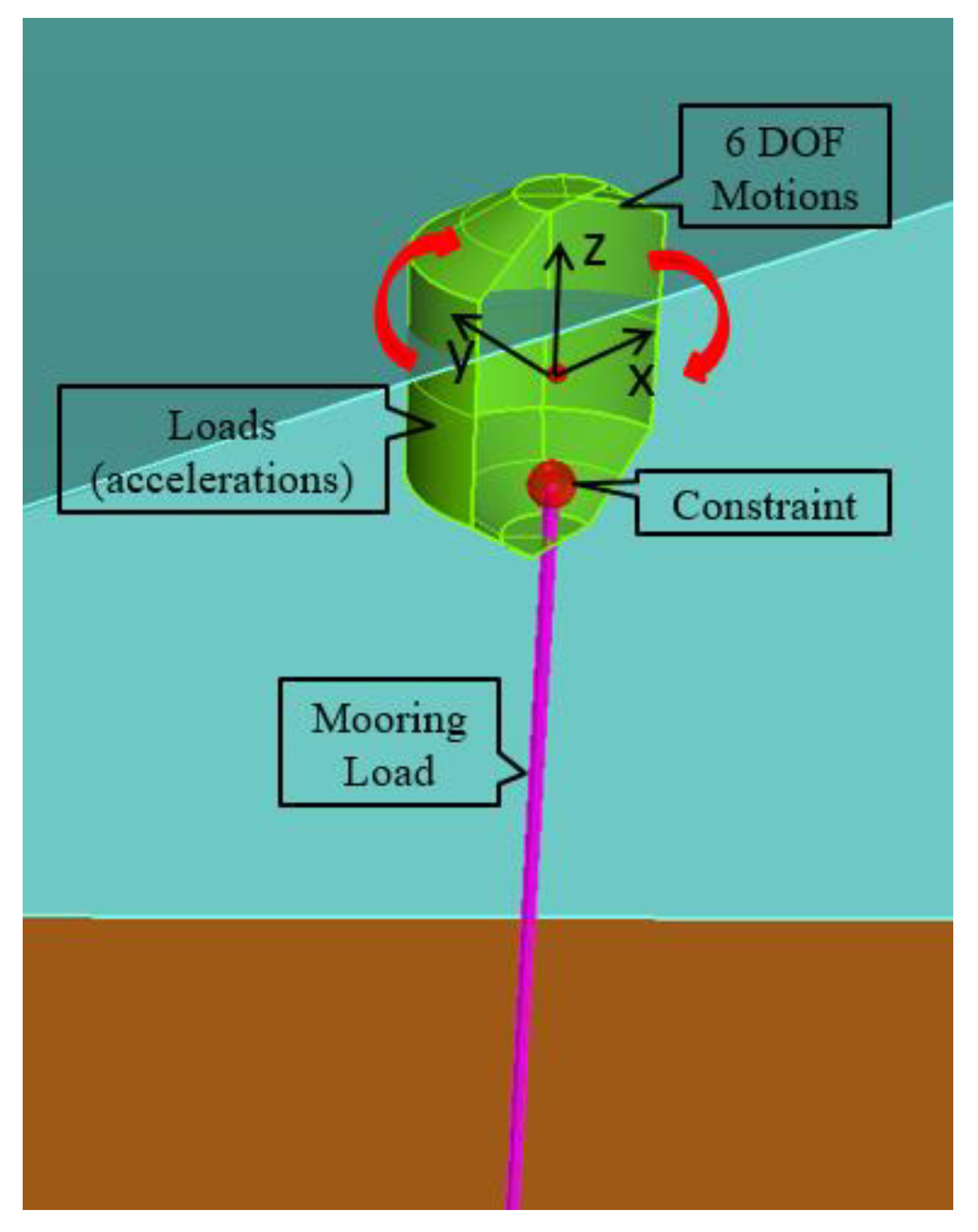
2.1. Coordinate Systems

To describe rigid body motions conveniently, two right-handed coordinate systems were used. The global coordinate system (GCS) is fixed to the earth (see Figure 1), a point of which is x = ( x , y , z ) . The local coordinate system (LCS) translates and rotates with the rigid body; a point in the LCS is x = ( x , y , z ) .
Vector ξ = ( ξ 1 , ξ 2 , ξ 3 ) represents the translation from the GCS origin (0,0,0) at the calm water line to the LCS origin ( ξ 1 , ξ 2 , ξ 3 ) . Rotation vector α = ( ξ 4 , ξ 5 , ξ 6 ) consists of the Euler angles between the GCS and the LCS. The coordinates in the LCS, x , are related to the coordinates in the GCS, x , through rotation matrix R :
x = R ( x ξ ) ,   R = [ c 5 c 6 ( c 4 s 6 + s 4 s 5 c 6 ) ( s 4 c 6 c 4 s 5 s 6 ) c 5 s 6 ( c 4 c 6 c 4 s 5 s 6 ) ( s 4 c 6 + c 4 s 5 s 6 ) s 5 s 4 c 5 c 4 c 5 ] .
In Equation ( 1 ) , c i represents c o s ( ξ i ) , and s i represents s i n ( ξ i ) . In SIMDYN, the order of rotation used was roll first, then pitch, and then yaw following the convention specified by Ogilvie [32]. The angular velocity in the GCS is ω = R T ω , where ω is the angular velocity in the LCS. If we express the angular velocity in the matrix form:
ω = [ 1 0 s 5 0 c 4 s 4 c 5 0 s 4 c 4 c 5 ] { α 1 ˙ α 2 ˙ α 3 ˙ } = Q α ˙   ω = [ c 5 c 6 s 6 0 c 5 s 6 c 6 0 s 5 0 1 ] { α 1 ˙ α 2 ˙ α 3 ˙ } = P α ˙ .
In this paper, ξ ˙ means the time derivative, and ξ ¨ means the second time derivative.

2.2. Governing Equations

The blended time-domain method is based on the nonlinear equations of motion. According to previous work [12], the exact equations of motion are as follows:
{ m [ ξ ¨ + ω ˙ × ( x G ξ ) + ω × [ ω × ( x G ξ ) ] ] = F I ω ˙ + ω × I ω = R [ M x G × F ] ,
where m is the mass, and I is the mass moment of inertia with respect to the center of gravity. The force in Equation ( 3 ) is applied at the center of gravity of the rigid body in the GCS. The moment in Equation ( 3 ) is with respect to the center of gravity of the rigid body in the LCS. The left hand side of Equation ( 3 ) are the inertia forces while the right-hand side are the external forces F (force at the center of gravity in the GCS) and moments M (the moment with respect to the origin of the GCS in the GCS):
{ W E C S i m : [ F , M ] T = F F K + F d i f + F r a d + F v i s + F h y d + F m o r + F m e + F P T O S I M D Y N :   [ F , M ] T = F F K + F d i f + F r a d + F v i s + F h y d + F m o r + F m e + F P T O + F s v .
The Sandia National Laboratory and the National Renewable Energy Laboratory developed WEC-Sim specifically to model a wave energy converter [33]. Compared to WEC-Sim, SIMDYN includes an additional force: slowly varying drift forces F s v (used under the linear time-domain option). The other forces are Froude-Krylov forces ( F F K ), diffraction forces ( F d i f ), radiation forces ( F r a d ), viscous forces ( F v i s ), hydrostatic forces ( F h y d ), forces from the mooring system ( F m o r ), Morison element forces ( F m e ), and power take-off (PTO) forces ( F P T O ).
Equation ( 4 ) includes the power take-off term to describe the program completely. However, in the simulations (linear and blended) performed for this paper, the PTO modeling is not used. This is because the floating power system in the model tests had no PTO, which helps reduce the uncertainty of model test correlations (to examine SIMDYN as a simulation tool).
The viscous forces, radiation forces, diffraction forces, and Morison forces can be calculated in the usual way adopted by any linear time-domain program (e.g., [7]). Table 2 compares several time-domain programs that can simulate WESs on the important forces that can be calculated differently.
The blended time-domain algorithm in SIMDYN is one of the tool’s most advanced features, including the nonlinear inertia forces (not applied in other programs shown in Table 2) and the drift forces (not applied in most other programs except in the commercial software AQWA).

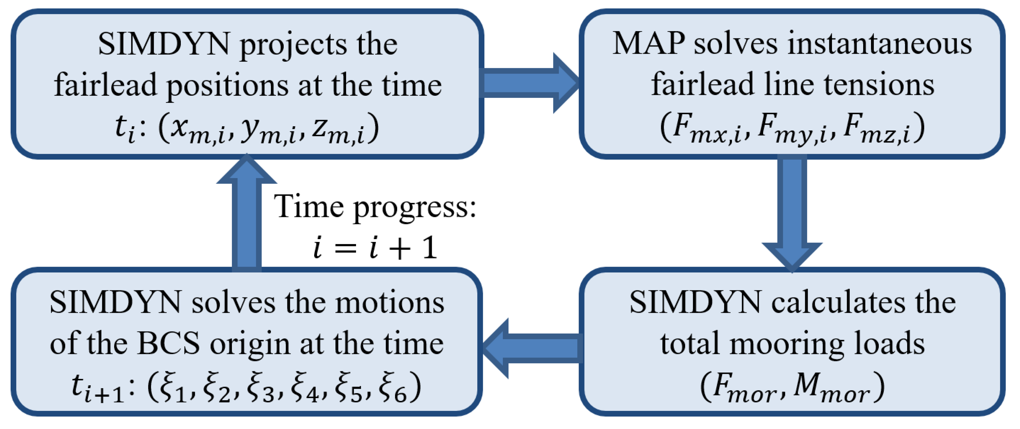
2.2.1. Mooring Forces/Moments

Mooring in SIMDYN is modeled using the open-source MAP++. MAP++ performs mooring analysis with quadratic modeling [27]. MAP++ ignores the inertia forces of the mooring lines and the fluid drag forces on the mooring lines [34]. Figure 2 shows how MAP++ is coupled with SIMDYN.
( F m x , i ,   F m y , i , F m z , i ) denotes the instantaneous fairlead translation forces of mooring line number i . The fairlead position of mooring line number i , x m , i = ( x m , i ,   y m , i ,   z m , i ) is projected from the origin of the body coordinate system, ( ξ 1 , ξ 2 , ξ 3 ) .

2.2.2. Slowly Varying Drift Forces/Moments

Slowly varying drift forces affect WES responses under irregular waves. Therefore, when the linear time-domain option is used, SIMDYN calculates the drift forces. In this study, the quadratic transfer functions were output from the Marine Dynamic Laboratory’s hydrodynamic analysis program, MDL-HydroD (a frequency domain program developed by our research group). Details on how quadratic transfer functions (QTFs) are evaluated can be found in previous work [35,36]. Figure 3 show sub-harmonic force quadratic transfer functions for surge and pitch.
If the random incident wave is decomposed as
η = i = 1 N F a i c o s ( ω i t + ϵ i ) .
The corresponding (second-order) slowly varying wave drift force are (see [7])
F s v ( t ) = i = 1 N F j = 1 N F [ a i a j P i j c o s ( ω t + ϵ ) + a i a j Q i j s i n ( ω t + ϵ ) ] .
The sum frequency components in the drift forces are neglected in the equation because their contributions are usually much smaller than the difference frequency components. a i , a j are the amplitude of the wave components with the frequency ω i and ω j and the phase ϵ i and ϵ j . ω = ω i ω j , ϵ = ϵ i ϵ j . N F is the number of frequency used to define the frequency range. P i j are the in-phase components of the quadratic transfer function for the difference frequency ω . Q i j are the out-of-phase components of the quadratic transfer function for difference frequency ω .

2.2.3. Viscous Forces/Moments

There are two terms related to viscous drag: F v i s and F m e . Either of them can be used in SIMDYN.
F v i s : SIMDYN can model the viscous forces using the linearized (equivalent) damping coefficient B e q :
F v i s = B e q ξ j ˙ ( t ) .
Alternatively, the viscous forces can be modeled in the quadratic form of
F D = 1 2 C d v ξ j ˙ ( t ) | ξ j ˙ ( t ) | .
C d v are the quadratic damping coefficients and ξ j ˙ is the jth degree of freedom velocity of the body’s center of gravity. The drag coefficients should be determined by model test correlations (e.g., free decay tests, system identification, empirical formula or data). Practically, it depends upon the user which degree of freedom they want to apply the damping to, and what are the appropriate damping values. For example, in SIMDYN:
*external_damping 4 1 4E4 → a linear viscous rolling damping of 4 × 10⁴ Ns/m is applied.
*quadratic_damping 1 2 2E3 → a quadratic viscous surge damping of 2 × 10³ Ns2/m2 is applied.

3. Nonlinear Froude-Krylov and Hydrostatic Forces

3.1. Formulation of Nonlinear Froude-Krylov and Hydrostatic Forces

In the blended time-domain method, Froude-Krylov forces are calculated by integrating the nonlinear dynamic pressure over the instantaneous wetted surface of the rigid body [25]. In this way, the method accounts for the effects of the instantaneous body motions and the instantaneous-incident free surface. Linear incident wave potential at point ( x ,   y ,   z ) in the GCS due to a unidirectional irregular sea incident at counterclockwise angle β to the body’s longitudinal axis is given by the following:
ϕ I = i = 1 N F H i g 2 ω i · c o s h [ k i ( h + z w ) ] cosh ( k i h ) s i n [ k i ( x c o s β + y s i n β ) ω i t ] .
For wave frequency component i , H i is the wave height, ω i is the frequency, k i is the wave number, h is the water depth, and N F is the total number of wave frequencies. The linear incident wave potential is not defined for the points above the mean water line ( z = 0 ) . SIMDYN employs Wheeler stretching to extrapolate the incident and hydrostatic pressure profiles to provide an expression for pressure inside the incident wave crest [37,38]. Mathematically, this can be considered as scaling the z-coordinate to compute pressure up to instantaneous free surface elevation η (measured from the calm water plane) due to the incident wave [37,38]. The vertical coordinate z is modified to z w through Wheeler stretching:
z w = h h + η ( t , x , y ) [ z η ( t , x , y ) ] .
Dynamic pressure p is as follows:
p ( t , x , y , z w ) = ρ ϕ I t ( t , x , y , z w ) ρ 2 | ϕ I ( t , x , y , z w ) | 2 .
Note that dynamic pressure ρ 2 | ϕ I ( t , x , y , z w ) | 2 is also nonlinear. The surface panels of the rigid body satisfying condition z η ( t , x , y ) form instantaneous wetted panels P B . The Froude-Krylov forces/moments are as follows:
F F K = P B   p ( t , x , y , z w ) · n d S ,   M F K = P B   p ( t , x , y , z w ) · ( x × n ) d S ,
where n is the normal vector of the panel, and x is the position vector of the wetted panel centroid (in the GCS). SIMDYN nonlinearly-integrates the results of a pre-processed potential problem solved under linear conditions
Like the Froude-Krylov forces, in the blended time-domain method, the hydrostatic forces and moments are also calculated by integrating the hydrostatic pressure over the instantaneous wetted surface area [23]:
{ F h y d = m g k ^ + P B   ρ g z · n d S M h y d = x G × ( m g k ^ ) + P B   ρ g z · ( x × n ) d S ,
where m g k ^ is the rigid body weight vector, and P B are the instantaneous wetted panels satisfying z η ( t , x , y ) . Note that the hydrostatic pressure, ρ g z , is calculated using the actual vertical coordinate z instead of z w . In this way, Equations ( 12 ) and ( 13 ) satisfy the dynamic free-surface boundary condition over the incident wave profile.

3.2. Nonlinear Effects of Froude=Krylov and Hydrostatic Forces

This section presents the nonlinear effects through the forced motion tests. The forced motion tests are important because:
(1)
The forced motion tests show the different forcing corresponding to the same (large) motions. That can indicate the motion (as the final result) differences in an implicit way;
(2)
Any simulation tool comes with limitations. The forced motion test avoids the problem by disabling modules not robust enough and not very relevant (for example, the mooring module is not the focus of this study);
(3)
The forced motion test is a control-variable test. It eliminates the effects of other forces, which makes the effect from each force component clearer.
The geometry used in these tests is a floating power system (its details are presented in Section 5) as plotted in Figure 4. The forced motion tests refer to a series of SIMDYN simulations that use the specified (forced) motion time series to study a force component (e.g., Froude-Krylov). In these tests, the same motion time series are input to SIMDYN. SIMDYN generates the same incident wave for the linear time-domain simulation and the blended time-domain simulation. This practice ensures that the body motions and wave elevations in the two types of simulations at any time instant are identical. The only variable in the forced motion tests is the method (linear or nonlinear) of modeling the Froude-Krylov and hydrostatic forces.
The body motions (from the linear time-domain simulation) under a regular wave of H = 1 m ,   T = 7.0 s are recorded as the reference motions, M 1 . The study used a (large-amplitude) regular wave of H = 5   m ,   T = 7.0   s , and the forced motions were set at five times the reference motions, 5 × M 1 . Note that the motions in the forced motion tests (except M 1 ) were not simulated but were specified (as input time series). This is quite a harsh condition (large wave and motions) for the FPS; therefore, nonlinear effects could be observed clearly.
Figure 5 compares the Froude-Krylov and hydrostatic heave forces. The hydrostatic heave forces from the two simulations are very close, while the Froude-Krylov heave forces show slight differences.
Figure 6 compares the Froude-Krylov and hydrostatic pitch moments. The Froude-Krylov and hydrostatic pitch moments show significant relevance to the nonlinear effects: as the wave and motion amplitude increase, the surge force, and pitch moment become more and more relevant to the nonlinear effects.
Figure 7 compares different sets of assumptions applied in the nonlinear method (upper) with the linear method (lower). The model in the two methods is subject to the same regular wave of H = 2.0   m ,   T = 6.0   s .
From Figure 7, the following can be found:
(1)
The instantaneous rotations of the structure are not addressed in the linear modeling, so the wetted surfaces and the corresponding pressures are different.
(2)
The instantaneous rotations of the structure are not addressed in the linear modeling, so the normal direction variation of each panel is not captured.
(3)
The translation motions of the structure are not captured in the linear method, so the wetted surfaces and the corresponding pressures are different. Note that the surge and sway influence the relative phase of the incident wave, so they also contribute to the differences.

4. Nonlinear Inertia Forces

4.1. Derivations of the Nonlinear Inertia Forces

For an irregular wave, the radiation forces are as follows [39]:
{ F r a d } = [ A ( ) ] { ξ ¨ } 0 [ h ( τ ) ] { ξ ˙ ( t τ ) } d τ ,
where [ A ( ) ] is the 6 × 6 added mass matrix at infinite frequency. We can write the following:
[ A ( ) ] = [ A 11 3 × 3 A 12 3 × 3 A 21 3 × 3 A 22 3 × 3 ] ,
where A 11 3 × 3 , A 12 3 × 3 , A 21 3 × 3 , and A 22 3 × 3 represent the four 3 × 3 blocks of the 6 × 6 added mass matrix [ A ( ) ] , and [ h ( τ ) ] is the 6 × 6 retardation function matrix corresponding to the frequency-dependent radiation damping. Note that in the blended time-domain method, acceleration term [ A ( ) ] { ξ ¨ } in Equation ( 14 ) should be moved to the left side of Equation ( 3 ) . The equations of motion become the following:
{ m { ξ ¨ + ω ˙ × ( x G ξ ) + ω × [ ω × ( x G ξ ) ] } + A 11 3 × 3 ξ ¨ + A 12 3 × 3 α ¨ = F I ω ˙ + ω × I ω + A 21 3 × 3 ξ ¨ + A 22 3 × 3 α ¨ = R [ M x G × F ] .
Angular velocities ω and ω defined in Equation ( 2 ) can be expressed in matrix form as shown below:
ω = Q α ˙ ,   ω = P α ˙ .
Differentiating Equation ( 17 ) , the angular accelerations are achieved ( ω ˙ in the LCS, ω ˙ in the GCS):
ω ˙ = Q α ¨ + Q ˙ α ˙ ,   ω ˙ = P α ¨ + P ˙ α ˙ .
Substituting Equations (17) and (18) into Equation (3) and rearranging to keep only the terms containing acceleration on the left side results in the following:
m ξ ¨ + A 11 3 × 3 ξ ¨ + m Q α ¨ × ( x G ξ ) + A 12 3 × 3 α ¨ = F m Q ˙ α ˙ × ( x G ξ ) m ω × [ ω × ( x G ξ ) ] .
Substituting Equations ( 17 )   to   ( 19 ) into Equation ( 16 ) yields the following:
I P α ¨ + I P ˙ α ˙ + A 21 3 × 3 ξ ¨ + A 22 3 × 3 α ¨ + P α ˙ × I P α ˙ = R M m R x G × ( Q α ¨ + Q ˙ α ˙ ) × ( x G ξ ) R { m x G × ξ ¨ + m x G × Q α ˙ × [ Q α ˙ × ( x G ξ ) ] + A 11 3 × 3 x G × ξ ¨ + A 12 3 × 3 x G × α ¨ } .
Equations ( 19 ) and ( 20 ) are rearranged into the matrix form. Let v denote a generic vector. Cross multiplication x G × v can be written in the matrix form:
x G × v = [ 0 x G 3 x G 2 x G 3 0 x G 1 x G 2 x G 1 0 ] { v 1 v 2 v 3 } = L 1 ( x G ) v .
Similarly, cross multiplication v × ( x G ξ ) can be written in the matrix form:
v × ( x G ξ ) = [ 0 x G 3 ξ 3 ( x G 2 ξ 2 ) ( x G 3 ξ 3 ) 0 x G 1 ξ 1 x G 2 ξ 2 ( x G 1 ξ 1 ) 0 ] { v 1 v 2 v 3 } = L 2 ( x G ξ ) v .
Using Equation ( 22 ) , ( 19 ) can be written as follows:
m ξ ¨ + A 11 3 × 3 ξ ¨ + m L 2 ( x G ξ ) Q α ¨ + A 12 3 × 3 α ¨ = F m L 2 ( x G ξ ) Q ˙ α ˙ m ω × [ L 2 ( x G ξ ) ω ] .
Substituting Equations ( 21 ) and ( 22 ) into Equation ( 20 ) and rearranging to keep only the terms containing acceleration on the left side results in the following:
m R L 1 ( x G ) ξ ¨ + R A 11 3 × 3 L 1 ( x G ) ξ ¨ + A 21 3 × 3 ξ ¨ + I P α ¨ + m R L 1 ( x G ) L 2 ( x G ξ ) Q α ¨ + A 22 3 × 3 α ¨ + R A 12 3 × 3 L 1 ( x G ) α ¨ = R M m R L 1 ( x G ) L 2 ( x G ξ ) Q ˙ α ˙ m R { L 1 ( x G ) Q α ˙ × [ L 2 ( x G ξ ) Q α ˙ ] } P α ˙ × I P α ˙ I P ˙ α ˙
In the matrix form, Equations ( 23 ) and ( 24 ) can be written as follows:
[ m + A 11 3 × 3 m L 2 ( x G ξ ) Q + A 12 3 × 3 m R L 1 ( x G ) + R A 11 3 × 3 L 1 ( x G ) + A 21 3 × 3 I P + m R L 1 ( x G ) L 2 ( x G ξ ) Q + A 22 3 × 3 + R A 12 3 × 3 L 1 ( x G ) ] { ξ ¨ α ¨ } = { F m L 2 ( x G ξ ) Q ˙ α ˙ m ω × [ L 2 ( x G ξ ) ω ] R M m R L 1 ( x G ) L 2 ( x G ξ ) Q ˙ α ˙ m R { L 1 ( x G ) Q α ˙ × [ L 2 ( x G ξ ) Q α ˙ ] } P α ˙ × I P α ˙ I P ˙ α ˙ }
Equation ( 25 ) is the nonlinear equation of motion used in SIMDYN; it can be solved using the fourth-order Runge–Kutta method [12].

4.2. Nonlinear Effects of the Inertia Force

This subsection presents the nonlinear effects of the inertia force (see also [40,41,42]) through forced motion tests on the FPS geometry shown in Figure 4. In Equation ( 16 ) , all the nonlinear terms are related to rotations. Note that Equation ( 16 ) includes the inertia forces due to the added masses on the left sides. Equation ( 16 ) can be rewritten as follows:
{ F = m [ ξ ¨ + ω ˙ × ( x G ξ ) + ω × [ ω × ( x G ξ ) ] ] + A 11 3 × 3 ξ ¨ + A 12 3 × 3 α ¨ M = R T ( I ω ˙ + ω × I ω + A 21 3 × 3 ξ ¨ + A 22 3 × 3 α ¨ ) + x G × F .
Using Equation ( 26 ) , nonlinear inertia forces F and moments M can be calculated. Note that in the linear time-domain method, the motions and rotations are assumed small:
x G x G , ω ω α ˙ , ω ˙ ω ˙ α ¨ ,
where x G are the coordinates of the center of gravity in the LCS, which are constant. Taking these assumptions to remove the nonlinear terms in Equation ( 25 ) , we obtain the following:
[ m + A 11 3 × 3 m L 2 ( x G ) + A 12 3 × 3 m L 1 ( x G ) + A 21 3 × 3 I + m L 1 ( x G ) L 2 ( x G ) + A 22 3 × 3 ] { ξ ¨ α ¨ } = { F M } .
Note that the terms containing L 1 ( x G ) and L 2 ( x G ) convert the momentum of inertia from the center of gravity to the origin of the LCS in the linear model, (0, 0, 0). This is the typical linear equation of motion. From Equation ( 28 ) , the linear inertia forces and moments can be calculated.
Using Equations ( 26 ) and ( 28 ) , the inertia forces in the forced motion tests (i.e., the time series of the motions, velocities, and accelerations are given) can be obtained. Note that the moments are given in the GCS from Equations ( 26 ) and ( 28 ) ; therefore, the inertia moments from the blended time-domain method should be transformed to the instantaneous origin of the body coordinate system, ( ξ 1 , ξ 2 , ξ 3 ) , to be compared with those from the linear time-domain method.
In the forced motion tests, the translational motions were set to zero to reveal the nonlinear effects due to the rotation. The first set of forced motions of the FPS are quite mild, referred to as M 2 (see Figure 8). M 2 is specified to show the inertia force differences (between the two options), so the relative phases of the rotations are not necessarily realistic.
The inertia forces corresponding to 10 times the reference motions, 10 × M 2 , are plotted in Figure 9. The surge and sway forces from the two methods are slightly different, indicating that the nonlinearity due to rotation is not significant at these rotation amplitudes.
The heave force from the blended model looks very different from the linear model but bear in mind that when the actual heave motion is in place, the contribution from the heave motion itself is much greater (>1000 times) than that from the rotations.
Under the forced rotations, 10 × M 2 , the differences in roll and pitch moments between the linear model and the blended model are noticeable (see Figure 10). The significant difference of the yaw moments indicates that for yaw, in this case, the linear model is no longer valid.
The blended results contain higher (mostly double) frequency components in sway, heave, yaw, and roll. They are the superharmonic components contributed by the nonlinear terms in the equation of motion. For example, in a case with zero yaw accelerations (an axisymmetric buoy), the combination of roll and pitch rotations will provide a nonlinear contribution to the yaw inertial forces using the nonlinear model.

5. Model Test Correlations

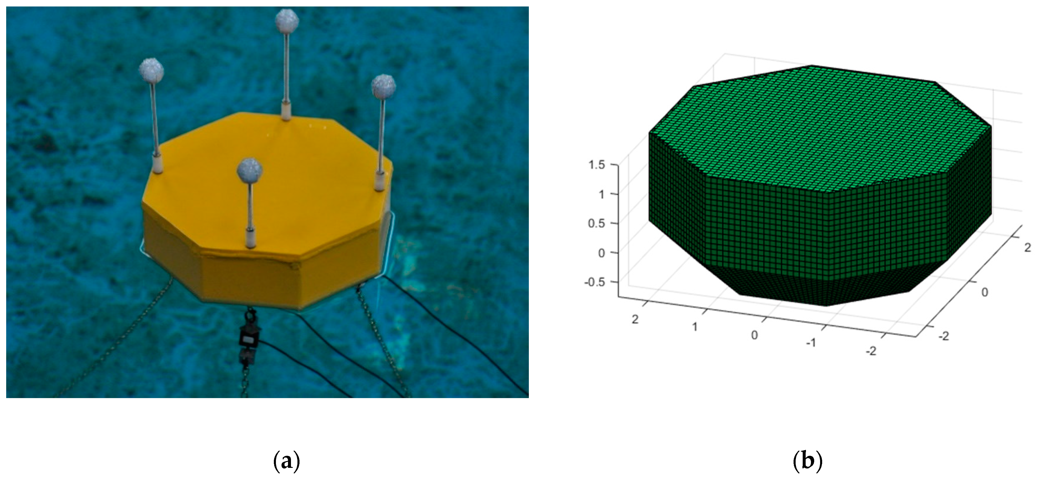
5.1. Model Test Setup and Input Information

The blended time-domain program SIMDYN (manufacturer, city and country) was examined using correlations with a series of 1:25-scale model tests [31] performed by Beaufort Research/HMRC in Ireland. In these model tests, the incident wave headings included 0°, 30°, and 60°. The 0° wave heading test was selected as it consists of more sea states. The 0° wave test configuration is shown in Figure 11.
The 0° wave heading tests consisted of 43 regular wave cases. There were 20 random (Bretschneider spectrum) wave cases with 0° wave heading, but some cases were skipped due to indications of incomplete measurements (over the time span of 1748 s) or unexpectedly large roll and yaw measurements (which should not be the case, as the configuration is symmetric about the x-axis). The unexpectedly large roll and yaw measurements may be partially attributed to parametric instabilities, which many wave-activated WECs suffer from (see [42,43,44,45,46,47,48,49,50]). These dynamic instabilities deserve systematic studies in the future. Consequently, 12 irregular wave cases were compared. The correlated sea states are plotted in Figure 12.
MDL-HydroD was used to perform the frequency domain analysis. The added masses, the radiation dampings, the diffraction forces, and the QTFs necessary for the blended time-domain analysis were obtained. More details about MDL-HydroD can be found in previous work [51,52,53,54].
Figure 13a shows the 1:25-scale FPS model used in the wave basin. The FPS panel model in Figure 13b was used in SIMDYN (for the integration of instantaneous pressure). The FPS has an octagon cross-section with a decreasing cross-section area below the calm water line. It consisted of 8,919 panels (see Figure 7), which proved fine enough to capture the nonlinear effects. The wetted surface was not re-meshed during the simulations. A panel is either fully submerged or fully emerged (by determining whether the instantaneous centroid of the panel is above/below the free surface). The FPS is positioned by a 3-leg catenary mooring system with a 120-degree azimuth difference between each mooring leg.
Table 3 lists the inputs used in the model test correlations. VCG is the vertical center of gravity and it is measured from the calm water plane (instead of from the bottom of the body). Kxx, Kyy, and Kzz are the gyration radius, around the center of gravity. EA is the element axial stiffness.

5.2. Correlations of the Regular Wave Cases

The FPS geometry and mooring system configuration was symmetric about the x-axis, so relative small sway, roll, and yaw motions were expected. The dominating surge, heave, and pitch motions from the time-domain (the linear and the blended) analysis were compared with the model tests.
Of the total 43 cases, 38 were successfully analyzed with reasonable time-series results. Typical cases are of the form similar to sinusoidal time history (as plotted in Figure 14 and Figure 15). From the plots, we can find both the linear model and the blended model to yield reasonable comparisons with the model tests (for surge and pitch). Motion amplitudes from the blended option look closer (than the linear model) as compared to the model test. The heave plots were omitted because the simulated heave motions were very close to the model test (no noticeable difference).
For the motion time series (longer than 10 min), their standard deviations represent the motion magnitudes. Therefore, the simulation errors are as follows:
E r r o r = ( s t d s i m s t d e x p ) / s t d e x p × 100 % .
Figure 16 compares the errors for surge, heave, and pitch. The range [−10%, 10%] bounds 95% of the error dots, meaning that both the linear model and the blended model were found to yield an acceptable error level. While the heave motion errors from the two models are similar, the blended model was found to yield lower surge and pitch motion errors compared with the linear model. The statistics in Table 4 also reflect this.
As listed in Table 4, the mean errors of the 38 regular wave cases from the blended method are consistently lower than the mean errors from the linear method for surge, heave, and pitch.
In the case that the large positive errors canceled out the large negative errors (meaning the mean errors did not represent the actual error levels), mean absolute errors are listed in Table 4 to reflect the level of error in another way. The mean absolute errors from the blended model also were shown to be lower than the mean absolute errors from the linear model, except for heave (which was very close).
Table 4 indicates that the blended time-domain method has a considerable improvement in accuracy. The advantage of the blended method can be credited to its capability to account for the nonlinearity in Froude-Krylov, hydrostatic, and inertia forces.
Depending on the computer’s CPU capability, the absolute calculation time of the two methods is subject to change. However, the relative speed is meaningful. For a simulation of 3 min in real-time, using a step of 0.1 s, there should be 1800 steps (number of steps should be the criteria here as the step itself is flexible). Under this setting, the blended method spends 19 times the simulation time of that spent by the linear method.
Some factors will influence the relative speed (e.g., the number of panels, the inclusion of the drift forces, ramp time setting). While the algorithm of the linear SIMDYN is quite mature, the algorithm of the blended SIMDYN has the room for more efficient optimization. In general, a fair estimation is that the blended time-domain method is about 10 times (one order of magnitude) slower than the linear time-domain method. Please remember that the next fidelity model (nonlinear time-domain method) is about 102 times (two orders of magnitude) slower than the linear time-domain method (see [5]).
Although the model test correlations in this paper show insignificant differences using the two modeling approaches. However, this happens when the linear method results are already fairly close to the model test results, leaving small room for improvements. We believe that under more severe sea states, or for better-tuned devices, the differences will be more significant.
For all the regular wave cases, the general trend of the response amplitude ratio (blended/linear) (including surge, heave, and pitch) is plotted in Figure 17.
From Figure 17a, we can find that (1) when the wave amplitude and motion amplitude are small, the blended method and the linear method are statistically very close and (2) as the wave and motion amplitude increase, the results from the linear method exceed the results from the blended method. The gradual loss of credibility of the linear assumptions with the increase of wave and motion amplitude leads to overprediction of the motions from the linear method. In addition, Figure 17b indicates that the accuracy of the blend method is quite consistent as the wave height changes.

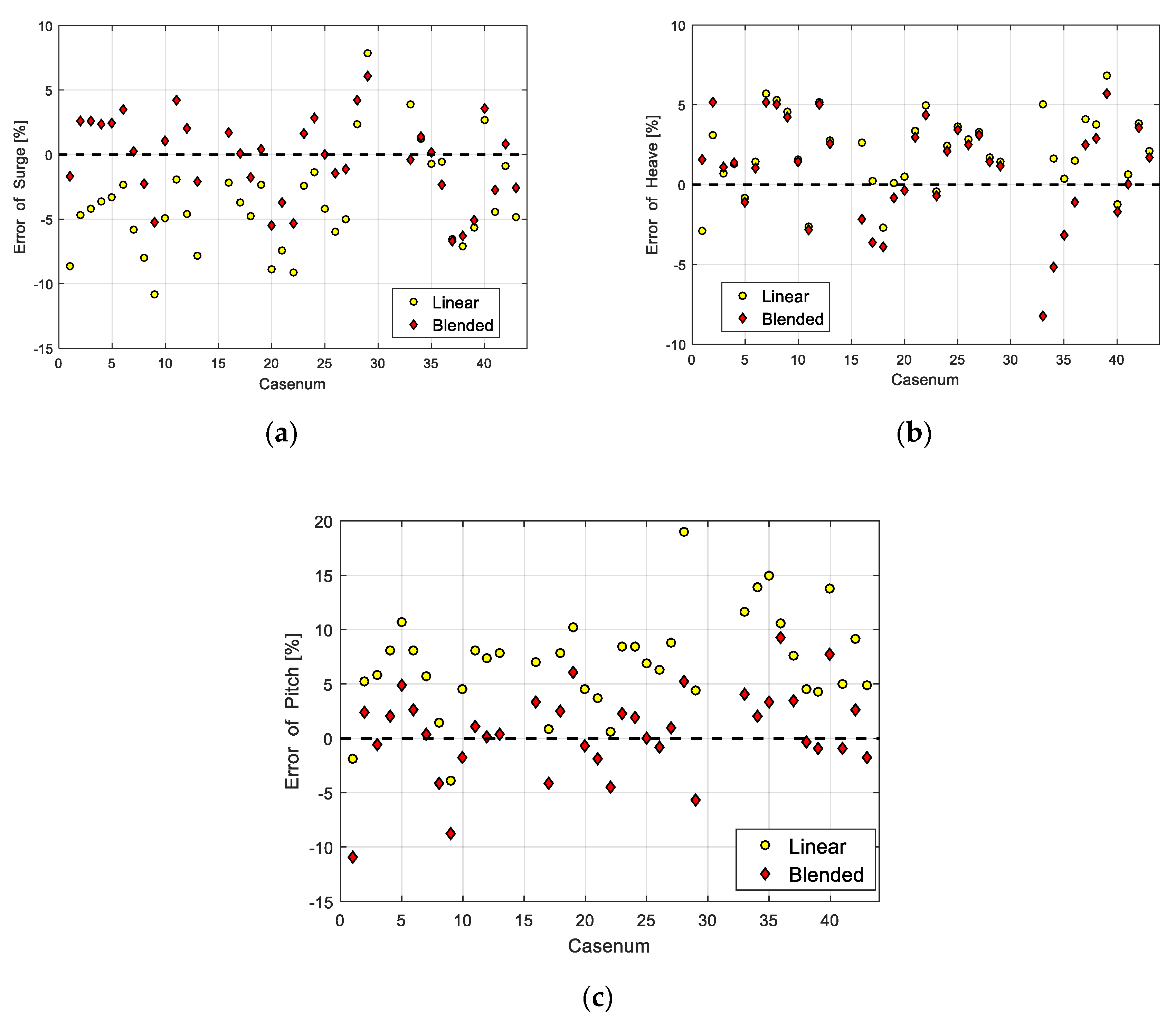
5.3. Correlations of Irregular Wave Cases

Similarly, the time-domain results of the selected irregular cases were compared with the model tests. Typical time series are plotted in Figure 18 and Figure 19.
From Figure 18 and Figure 19, we can observe reasonable correlations between the simulations and the model tests. However, as the irregular wave cases were more complex, the close matches of the time series (similar to what we obtained in Figure 14 and Figure 15 in the regular wave cases) were not available in the irregular wave cases. However, the typical heave motions (see Figure 20) correlated better (with the model tests) than the typical surge and pitch motions shown in Figure 18 and Figure 19.
The motion errors from the two methods are listed in Table 5. The errors from the blended time-domain model are also lower.

6. Discussion

The blended, weakly nonlinear time-domain method was implemented to predict WES motions. This method calculates important external forces by directly integrating the instantaneous pressure on the wetted panels of the floating structures, while the remaining external forces are processed in ways adopted by traditional linear time-domain programs (e.g., OrcaFlex). The method also accounts for nonlinearity in the equations of motion (i.e., inertia forces) due to rotations of the rigid body. The simulation results from the blended time-domain method were compared with the experimental results measured under the same incident waves. Correlations with the model test results indicate that the blended time-domain method is more accurate than the widely used linear time-domain method as it reduces the error of the motion responses. Moreover, the method is significantly faster than possibly more exact methods such as fully nonlinear time-domain methods or CFD.
This study also discussed the nonlinear effects of Froude-Krylov, hydrostatic, and inertia forces. The (forced) motion time series were input to both the linear model and the blended model to compare the corresponding Froude-Krylov, hydrostatic, and inertia forces. As in the forced motion tests, the method used (linear or blended) was the only variable, so the differences between the two methods under certain motion and wave amplitude could be compared. In general, the gap between the blended method and the linear method widens as the motion amplitude and wave amplitude increase. While the model test results generally compare well with both the linear and blended time-domain methods under the tested sea states, we reasonably deduce from the forced motion test results that with larger wave amplitudes, the advantages of the blended method may increase substantially.
In this work, a floating power system was used in the model test correlations. This geometry (selected from a very limited suitable model test data accessible to us), though not a real wave energy converter, is of dimensions and geometry similar to the typical point absorber type wave energy converter. At the stage of motion predictions through numerical modeling, especially under relatively large sea states, the WEC is usually in survival mode (when its PTO is deactivated). Therefore, for this study, the floating power system is almost equivalent to a point absorber type WEC. From this study, the blended method was found to be more accurate for the point absorber type WEC that usually undergoes large (relative to their dimensions) wave and motion amplitudes.
At this stage, the focus is to make sure that the motion predictions from the numerical modeling under different sea states are accurate. Even with the real wave energy converter, for this study (examining the modeling method under different sea states), it is preferable that the power take-off is deactivated. That makes the floating power system similar to the point absorber in essence. Actually, the improvements of SIMDYN and the confidences/benchmarks gained in this study are the foundation for any further study. In the future study, the power take-off forces will be activated in our model to simulate the point absorber in their working mode. That should produce better results for predicting the WEC’s electrical outputs (e.g., voltage, current and power). The refined motion predictions will not only improve the power take-off predictions for the WEC’s working mode but will also improve (more greatly) the load predictions for the point absorber type WEC’s survival mode. The more accurate motion predictions from our improved model can be directly used to determine the local accelerations (will determine the loads and pressures) as well as the mooring line tensions and offsets, which are the most critical quantities for designing WECs. Loads under extreme sea states are the key to overcoming risks and reducing costs of the point absorber type WECs, especially before their practical applications become more extensive.

7. Conclusions

(1)
A simulation program, SIMDYN, was developed using both the linear and the blended time-domain methods to predict the motions (six degrees of freedom) of the wave energy converters.
(2)
The nonlinear Froude-Krylov and hydrostatic forces were implemented in SIMDYN. The (dominant) external forces can be calculated more accurately without requiring significantly more calculation time.
(3)
The nonlinear inertia effects were addressed, which were usually neglected in the time domain analysis. They may prove to be as important as the nonlinear effects of the external forces.
(4)
The study also filled the gap in that the blended method has seldom been correlated with WES model tests. The comparisons between the simulations and the model tests were improved by the blended method.
(5)
The working mode modeling of the (point absorber type) WEC will benefit from the blended time-domain method’s more accurate motion predictions.
(6)
The survival mode (under large sea states) modeling of the (point absorber type) WEC can be greatly improved using the blended time-domain method without increasing the calculation time several orders of magnitude of as would occur using a fully nonlinear time-domain program or a CFD program.

Author Contributions

Conceptualization, H.W., A.S. and J.F.; data curation, H.W.; formal analysis, H.W. and Z.X.; funding acquisition, J.F.; investigation, H.W. and J.F.; methodology, H.W., A.S. and J.F.; software, H.W. and A.S.; supervision, J.F.; validation, H.W. and A.S.; visualization, H.W.; writing—original draft, H.W.; writing—review and editing, H.W., A.S., J.F., and Z.X. All authors have read and agreed to the published version of the manuscript.

Funding

This research received no external funding.

Acknowledgments

The authors really appreciate the Beaufort Research/HMRC for providing the model test data and Bret Bosma for interpreting these data. The open-source mooring modeling program developed by Marco Masciola, MAP++, contributes as an essential component in the simulation program. Suggestions provided by Yi-Hsiang Yu and Jason Jonkman from the National Renewable Energy Laboratory are also useful additions to our study.

Conflicts of Interest

The authors declare no conflict of interest.

References

  1. Falcão, A.F. Wave energy utilization: A review of the technologies. Renew. Sustain. Energy Rev. 2010, 14, 899–918. [Google Scholar] [CrossRef]
  2. Lópeza, I.; Andreu, J.; Ceballos, S.; Alegría, I.; Kortabarria, I. Review of wave energy technologies and the necessary power-equipment. Renew. Sustain. Energy Rev. 2013, 27, 413–434. [Google Scholar] [CrossRef]
  3. Lettenmaier, T.; Amon, E.; Jouanne, A. Power converter and control system developed in the ocean sentinel instrumentation buoy for testing wave energy converters. In Proceedings of the 3rd IEEE Energy Conversion Congress and Exposition, Denver, CO, USA, 15–19 September 2013. [Google Scholar]
  4. Coe, R.G.; Neary, V.S.; Lawson, M.; Yu, Y.H.; Weber, J. Extreme Conditions Modelling Workshop Report; The National Renewable Energy Laboratory: Golden, CO, USA, 2014.
  5. Yu, Y.H. WEC-Sim, a Time-Domain Numerical Model Development, Verification and Validation; National Renewable Energy Laboratory: Golden, CO, USA, 2017.
  6. Det Norske Veritas. Environmental Conditions and Environmental Loads, Recommended Practice; DNV-RP-C205; Det Norske Veritas: Oslo, Norway, 2007. [Google Scholar]
  7. ANSYS Inc. AQWA-DRFT User Manual; ANSYS Inc.: Houston, TX, USA, 2013. [Google Scholar]
  8. WAMIT Inc. WAMIT User Manual Version 7.0; WAMIT, Inc.: Chestnut Hill, MA, USA, 2013. [Google Scholar]
  9. Penalba, M.; Kelly, T.; Ringwood, J.V. Using NEMOH for modelling wave energy converters: A comparative study with WAMIT. In Proceedings of the 12th European Wave and Tidal Energy Conference, Cork, Ireland, 27 August–2 September 2017. [Google Scholar]
  10. Reed, A.; Beck, R. Advances in the predictive capability for ship dynamics in extreme waves. In Proceedings of the Society of Naval Architects and Marine Engineers Maritime Convention, Bellevue, Washington, DC, USA, 1–5 November 2016. [Google Scholar]
  11. The National Renewable Energy Laboratory and Sandia Corporation. WEC-Sim User Guide Version 1.0; 11.t National Renewable Energy Laboratory and Sandia Corporation: Golden, CO, USA, 2014.
  12. Somayajula, A.; Falzarano, J. Large-amplitude time-domain simulation tool for marine and offshore motion prediction. Mar. Syst. Ocean Technol. 2015, 10, 1–17. [Google Scholar] [CrossRef]
  13. Stern, F.; Carrica, P.; Kandasamy, M.; Ooi, S.K.; Fu, T.Z.J.; Hendrix, D.; Kennell, C.; Hughes, M.G.; Miller, R.; Marino, T.; et al. Computational Hydrodynamic Tools for High-speed Sealift: Phase II Final Report; The University of Iowa: Iowa City, IA, USA, 2008. [Google Scholar]
  14. Yu, Y.H.; Rij, J.; Coe, R.; Lawson, M. Preliminary wave energy converters extreme load analysis. In Proceedings of the 34th International Conference on Ocean, Offshore and Arctic Engineering, St. John’s, NL, Canada, 31 May–5 June 2015. [Google Scholar]
  15. Yeylaghi, S.; Moa, B.; Beatty, S.; Buckham, B.; Oshkai, P.; Crawford, C. SPH modelling of hydrodynamic loads on a point absorber wave energy converter hull. In Proceedings of the 11th European Wave and Tidal Energy Conference, Nantes, France, 6–11 September 2015. [Google Scholar]
  16. Sagaut, P. Large Eddy Simulation for Incompressible Flows: An Introduction; Springer: New York, NY, USA, 2006. [Google Scholar]
  17. CD-adapco. User Guide STAR-CCM+ Version 9.04; CD-adapco: Melville, NY, USA, 2014. [Google Scholar]
  18. OpenFOAM Foundation Ltd. OpenFOAM User Guide; OpenFOAM Foundation Ltd.: London, UK, 2019. [Google Scholar]
  19. Lawson, M.; Garzon, B.B.; Wendt, F.; Yu, Y.H.; Michelen, C. COER hydrodynamic modelling competition: Modelling the dynamic response of a floating body using the WEC-Sim and FAST simulation tools. In Proceedings of the ASME 2015 34th International Conference on Ocean, Offshore and Arctic Engineering, St. John’s, NL, Canada, 31 May–5 June 2015. [Google Scholar]
  20. Umeda, N.; Hashimoto, H.; Tsukamoto, I.; Sogawa, Y. Estimation of parametric roll in random seaway. In Parametric Resonance in Dynamical Systems; Fossen, T.I., Nijmeijer, H., Eds.; Springer: New York, NY, USA, 2012; pp. 45–59. [Google Scholar]
  21. Belenky, V.L.; Weems, K.M.; Lin, W.M.; Paulling, J.R. Probabilistic analysis of roll parametric resonance in head seas. In Proceedings of the 8th International Conference on Stability of Ships and Ocean Vehicles, Madrid, Spain, 15–19 September 2003. [Google Scholar]
  22. Chen, X. Studies on Dynamic Interaction between Deep-water Floating Structures and Their Mooring/tendon System. Ph.D. Thesis, Texas A&M University, College Station, TX, USA, 2002. [Google Scholar]
  23. Lawson, M.; Yu, Y.H.; Nelessen, A.; Ruehl, K.; Michelen, C. Implementing nonlinear buoyancy and excitation forces in the WEC-Sim wave energy converter modelling tool. In Proceedings of the 33rd International Conference on Ocean, Offshore and Arctic Engineering, San Francisco, CA, USA, 8–13 June 2014. [Google Scholar]
  24. Beck, R.F.; Reed, A.M. Modern computational methods for ships in a seaway. SNAME Trans. 2001, 109, 1–51. [Google Scholar]
  25. Penalba, M.; Giorgi, G.; Ringwood, J. Mathematical modelling of wave energy converters: A review of nonlinear approaches. Renew. Sustain. Energy. Rev. 2017, 78, 1188–1207. [Google Scholar] [CrossRef] [Green Version]
  26. Ransley, E.J.; Greaves, D.; Raby, A.; Simmonds, D.; Hann, M. Survivability of wave energy converters using CFD. Renew. Energy 2017, 109, 235–247. [Google Scholar] [CrossRef] [Green Version]
  27. MAP++ Documentation Release1.15. Available online: https://map-plus-plus.readthedocs.io/en/latest (accessed on 3 January 2019).
  28. Wang, H.; Falzarano, J. Energy balance analysis method in oscillating type wave converter. J. Ocean Eng. Mar. Energy 2017, 3, 193–208. [Google Scholar] [CrossRef]
  29. Sirnivas, S.; Yu, Y.H.; Hall, M.; Bosma, B. Coupled mooring analyses for the WEC-SIM wave energy converter design tool. In Proceedings of the ASME 2016 35th International Conference on Ocean, Offshore and Arctic Engineering, Busan, Korea, 19–24 June 2016. [Google Scholar]
  30. Ruehl, K.; Michelen, C.; Bosma, B.; Yu, Y.H. WEC-Sim Phase 1 validation testing: Numerical modelling of experiments. In Proceedings of the International Conference on Offshore Mechanics and Arctic Engineering, Busan, Korea, 19–24 June 2016. [Google Scholar]
  31. Bosma, B.; Sheng, W.; Thiebaut, F. Performance assessment of a floating power system for the Galway Bay wave energy test site. In Proceedings of the 5th International Conference on Ocean Energy, Halifax, NS, Canada, 4–6 November 2014. [Google Scholar]
  32. Ogilvie, T. Second-order hydrodynamic effects on ocean platforms. In International Workshop on Ship and Platform Motions; UC Berkeley: Berkley, CA, USA, 1983. [Google Scholar]
  33. WEC-Sim Documentation. Available online: https://wec-sim.github.io/WEC-Sim/index.html (accessed on 31 April 2019).
  34. Masciola, M.; Jonkman, J.; Robertson, A. Implementation of a multisigmented, quasi-static cable mode. In Proceedings of the 23rd International Offshore and Polar Engineering Conference, Anchorage, AK, USA, 30 June–5 July 2013. [Google Scholar]
  35. Somayajula, A.; Falzarano, J. A comparative assessment of approximate methods to simulate second order roll motion of FPSOs. Ocean Syst. Eng. 2017, 7, 53–74. [Google Scholar] [CrossRef]
  36. Xie, Z.; Liu, Y.; Falzarano, J. A numerical evaluation of the quadratic transfer function for a floating structure. In Proceedings of the ASME 2019 38th International Conference on Ocean, Offshore and Arctic Engineering, Glasgow, UK, 9–14 June 2019. [Google Scholar]
  37. OrcaFlex Documentation. Available online: http://www.orcina.com/Software/Products/OrcaFlex/Documentation/Help (accessed on 5 February 2019).
  38. Giorgi, G.; Ringwood, J.V. Relevance of pressure field accuracy for nonlinear Froude-Krylov force calculations for wave energy devices. J. Ocean Eng. Mar. Energy 2018, 4, 57–71. [Google Scholar] [CrossRef] [Green Version]
  39. Cummins, W. The Impulse Response Function and Ship Motions; Technical Report; David Taylor Model Basin: Washington, DC, USA, 1962. [Google Scholar]
  40. Giorgi, G.; Ringwood, J.V. A Compact 6-DoF Nonlinear Wave Energy Device Model for Power Assessment and Control Investigations. IEEE Trans. Sustain. Energy 2018, 10, 119–126. [Google Scholar] [CrossRef]
  41. Giorgi, G.; Ringwood, J.V. Analytical representation of nonlinear Froude-Krylov forces for 3-DoF point absorbing wave energy device. Ocean Eng. 2019, 164, 749–759. [Google Scholar] [CrossRef] [Green Version]
  42. Tarrant, K.; Meskell, C. Investigation on parametrically excited motions of point absorbers in regular waves. Ocean Eng. 2016, 111, 67–81. [Google Scholar] [CrossRef]
  43. Babarit, A.; Mouslim, H.; Clément, A.; Laporte-Weywada, P. On the numerical modelling of the nonlinear behaviour of a wave energy converter. In Proceedings of the 28th International Conference on Ocean, Offshore and Arctic Engineering, Honolulu, HI, USA, 31 May–5 June 2009. [Google Scholar]
  44. Giorgi, G.; Ringwood, J.V. Articulating parametric resonance for an OWC spar buoy in regular and irregular waves. J. Ocean Eng. Mar. Energy 2018, 4, 311–322. [Google Scholar] [CrossRef]
  45. Kurniawan, A.; Grassow, M.; Ferri, F. Numerical modelling and wave tank testing of a self-reacting two-body wave energy device. Ships Offshore Struct. 2019, 14, 344–356. [Google Scholar] [CrossRef]
  46. Palm, J.; Eskilsson, C.; Bergdahl, L. Parametric excitation of moored wave energy converters using viscous and non-viscous CFD simulations. In Proceedings of the 3rd International Conference on Renewable Energies Offshore, Lisbon, Portugal, 8–10 October 2018. [Google Scholar]
  47. Gomes, R.P.F.; Ferreira, J.D.C.M.; Silva, S.R.; Henriques, J.C.C.; Gato, L.M.C. An experimental study on the reduction of the dynamic instability in the oscillating water column spar buoy. In Proceedings of the 12th European Wave and Tidal Energy Conference, Cork, Ireland, 27 August–1 September 2017. [Google Scholar]
  48. Orszaghova, J.; Wolgamot, H.; Draper, S.; Eatock Taylor, R.; Taylor, P.H.; Rafiee, A. Transverse motion instability of a submerged moored buoy. Proc. R. Soc. A Math. Phys. Eng. Sci. 2019, 475. [Google Scholar] [CrossRef] [PubMed] [Green Version]
  49. Orszaghova, J.; Wolgamot, H.; Draper, S.; Rafiee, A. Motion instabilities in tethered buoy WECs. In Proceedings of the 4th Asian Wave and Tidal Energy Conference, Taipei, China, 9–13 September 2018. [Google Scholar]
  50. Orszaghova, J.; Wolgamot, H.; Eatock Taylor, W.; Draper, S.; Rafiee, A.; Taylor, P.H. Simplified dynamics of a moored submerged buoy. In Proceedings of the 32nd International Workshop on Water Waves and Floating Bodies, Dalian, China, 23–26 April 2017. [Google Scholar]
  51. Guha, A. Development and Application of a Potential Flow Computer Program: Determining First and Second Order Wave Forces at Zero and Forward Speed in Deep and Intermediate Water Depth. Ph.D. Thesis, Texas A&M University, College Station, TX, USA, 2016. [Google Scholar]
  52. Liu, Y.; Falzarano, J. Suppression of irregular frequency effect in hydrodynamic problems and free-surface singularity treatment. J. Offshore Mech. Arct. Eng. 2017, 139, 1–16. [Google Scholar] [CrossRef]
  53. Guha, A.; Falzarano, J. Development of a computer program for three dimensional analysis of zero speed first order wave body interaction in frequency domain. In Proceedings of the ASME 2013 32nd International Conference on Ocean, Offshore and Arctic Engineering, Nantes, France, 9–14 June 2013. [Google Scholar]
  54. Guha, A.; Falzarano, J. The effect of hull emergence angle on the near field formulation of added resistance. Ocean Eng. 2015, 105, 10–24. [Google Scholar] [CrossRef]
Figure 1. Generic wave energy structure.
Jmse 08 00001 g001
Figure 2. Coupling of SIMDYN and MAP++.
Jmse 08 00001 g002
Figure 3. (a) Surge quadratic transfer function (QTF); (b) pitch QTF.
Jmse 08 00001 g003
Figure 4. Geometry of a floating power system.
Jmse 08 00001 g004
Figure 5. Heave forces ( H = 5   m ,   T = 7.0   s , motions 5 × M 1 ): (a) Froude–Krylov; (b) hydrostatic.
Jmse 08 00001 g005
Figure 6. Pitch moments ( H = 5   m ,   T = 7.0   s , motions 5 × M 1 ): (a) Froude–Krylov; (b) hydrostatic.
Jmse 08 00001 g006
Figure 7. Floating power system (FPS) modeling (upper: nonlinear modeling, lower: linear modeling).
Jmse 08 00001 g007
Figure 8. Reference forced motions M 2 .
Jmse 08 00001 g008
Figure 9. Translation inertia forces corresponding to forced motion 10 × M 2 .
Jmse 08 00001 g009
Figure 10. Rotation inertia moments corresponding to forced motions 10 × M 2 .
Jmse 08 00001 g010
Figure 11. 0° wave test (with permission from the Beaufort Research/HMRC, 2014).
Jmse 08 00001 g011
Figure 12. Correlated sea states.
Jmse 08 00001 g012
Figure 13. Floating power system models: (a) floating power system tested in the wave basin (with permission from the Beaufort Research/HMRC, 2014); (b) floating power system (panel model) analyzed by the Marine Dynamic Laboratory.
Jmse 08 00001 g013
Figure 14. Motion comparisons for H = 1.0 m, T = 7.0 s: (a) surge; (b) pitch.
Jmse 08 00001 g014
Figure 15. Motion comparisons for H = 3.0 m, T = 9.0 s: (a) surge; (b) pitch.
Jmse 08 00001 g015
Figure 16. Regular wave case errors: (a) surge; (b) heave; (c) pitch.
Jmse 08 00001 g016
Figure 17. Response ratio: (a) blended/linear; (b) blended/experimental.
Jmse 08 00001 g017
Figure 18. Motion comparisons for Hs = 1.75 m, Tp = 8.5 s: (a) surge motions; (b) pitch motions.
Jmse 08 00001 g018
Figure 19. Motion comparisons for Hs = 1.75 m, Tp = 10.0 s: (a) surge motions; (b) pitch motions.
Jmse 08 00001 g019
Figure 20. Similar heave response from the experiments and the simulations.
Jmse 08 00001 g020
Table 1. Summary of hydrodynamic modeling method.
MethodHydrodynamicsSoftware
1Morison’s Equation [6]N/A
2Linear time (frequency) domain potential flow [7]AQWA [7], WAMIT [8], Nemoh [9]
3Blended time-domain potential flow [10]WEC-Sim [11], SIMDYN [12]
4Nonlinear time-domain potential flow [13]Aegir [13]
5Computation Fluid Dynamics (RANS [14], SPH [15], LES [16])STAR-CCM+ [17], OpenFoam [18]
6Model tests [19] (Physical modeling)N/A
Table 2. Comparison of time-domain programs (for modeling wave energy structures (WESs)).
Code NameAQWAWaveDynWEC-SimSIMDYN
DeveloperANSYS Inc.DNV GLSNL & NRELMDL
Froude-KrylovLinear, NonlinearLinear, Nonlinear Linear, Nonlinear Linear, Nonlinear
HydrostaticsLinear, NonlinearLinear, NonlinearLinear, NonlinearLinear, Nonlinear
Inertia ForcesLinearLinearLinearNonlinear
Drift ForcesFull QTFN/AN/AFull QTF
LicenseCommercialCommercialOpen-SourceResearch
Table 3. Floating power system information.
CharacteristicValueCharacteristicValue
Mass M (kg)11,337.9Anchor vertical position (m)−25.0
Length Lpp (m)5.00Anchor horizontal position (m)65.0
Breadth B (m)5.00Mooring line length (m)75.0
Height D (m)2.25Mass/unit length (kg/m)28.438
VCG (m)0.64Mooring line diameter (m)0.15
Kxx (m)1.386Added mass coefficient1.0
Kyy (m)1.386Transverse drag coefficient1.0
Kzz (m)1.821Longitudinal drag coefficient0.025
Draft T (m)0.75EA (N/m)1.0 × 108
Water depth h (m)25.0Maximum tension (kN)100.0
Fairlead vertical position (m)−0.75Number of mooring lines3
Fairlead horizontal position (m)1.5Line azimuth difference (°)120
Table 4. Comparisons of error for regular wave cases (38 cases).
ItemSurgeHeavePitch
MeanLinear−3.7%2.0%7.0%
Blended−0.3%1.0%0.5%
Mean of AbsLinear4.7%2.6%7.3%
Blended2.6%2.8%3.1%
Table 5. Comparisons of error for irregular wave cases (nine cases).
ItemSurgeHeavePitch
MeanLinear−13.8%0.7%4.3%
Blended−9.5%0.7%−1.0%
Mean of AbsLinear13.8%0.7%6.9%
Blended10.2%0.7%8.1%

