Model-Based Evaluation of Hydroelectric Dam’s Impact on the Seasonal Variabilities of POC in Coastal Ocean: A Case Study of Three Gorges Project

Abstract
:1. Introduction
2. Model and Data
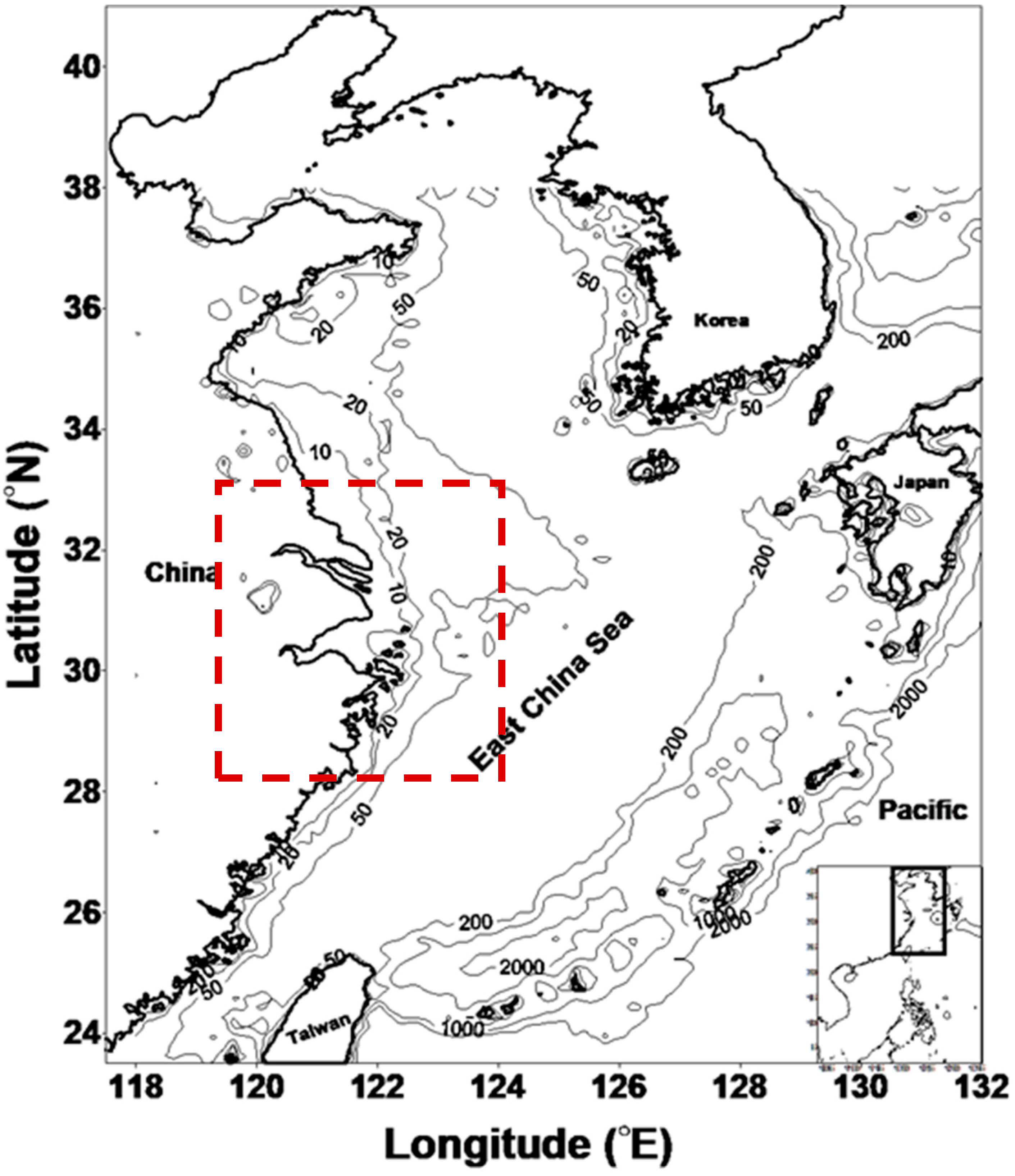
2.1. Physical Model
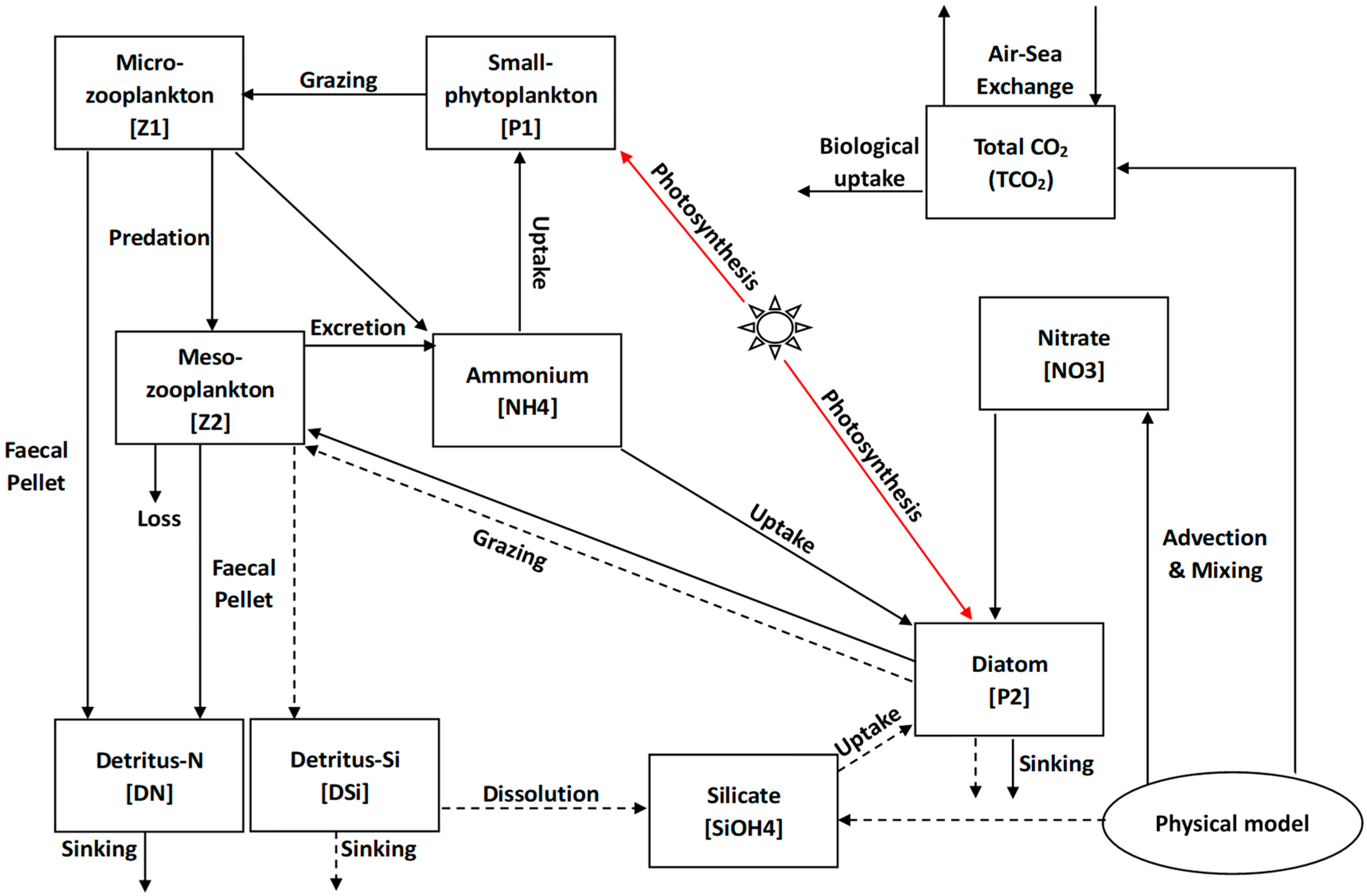
2.2. Ecosystem Model
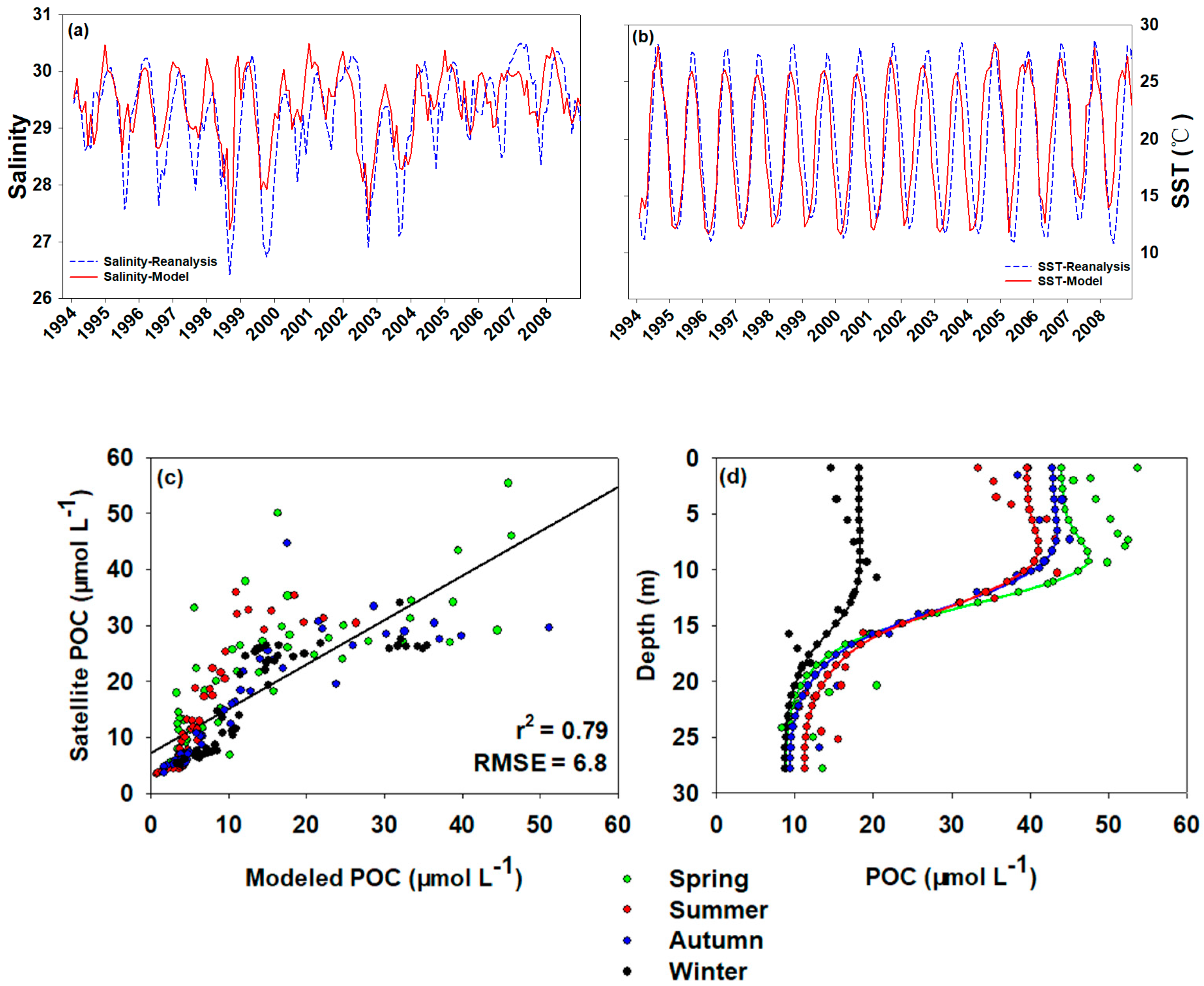
2.3. Model Validation
3. Results and Discussion
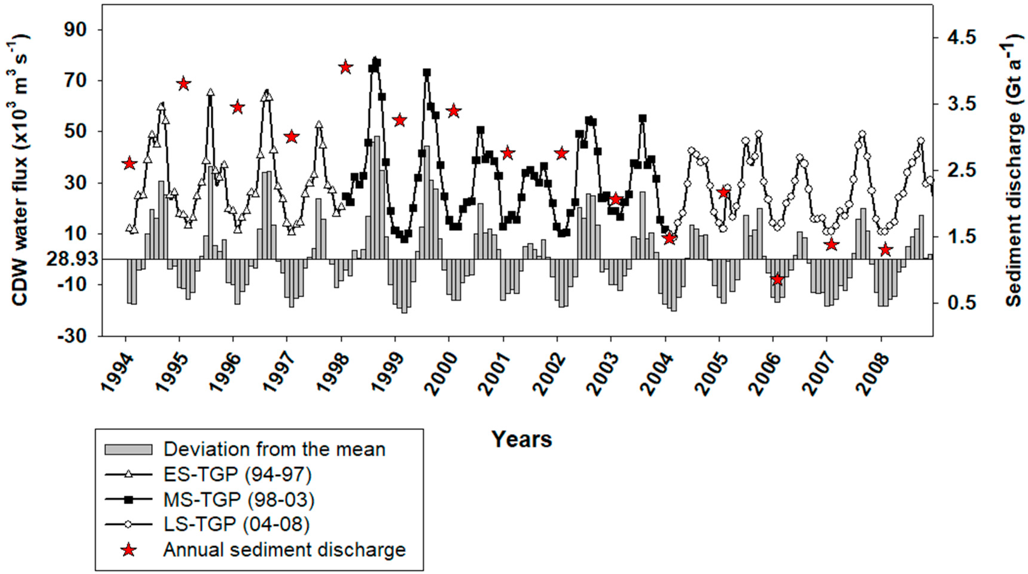
3.1. River and Sediment Discharge
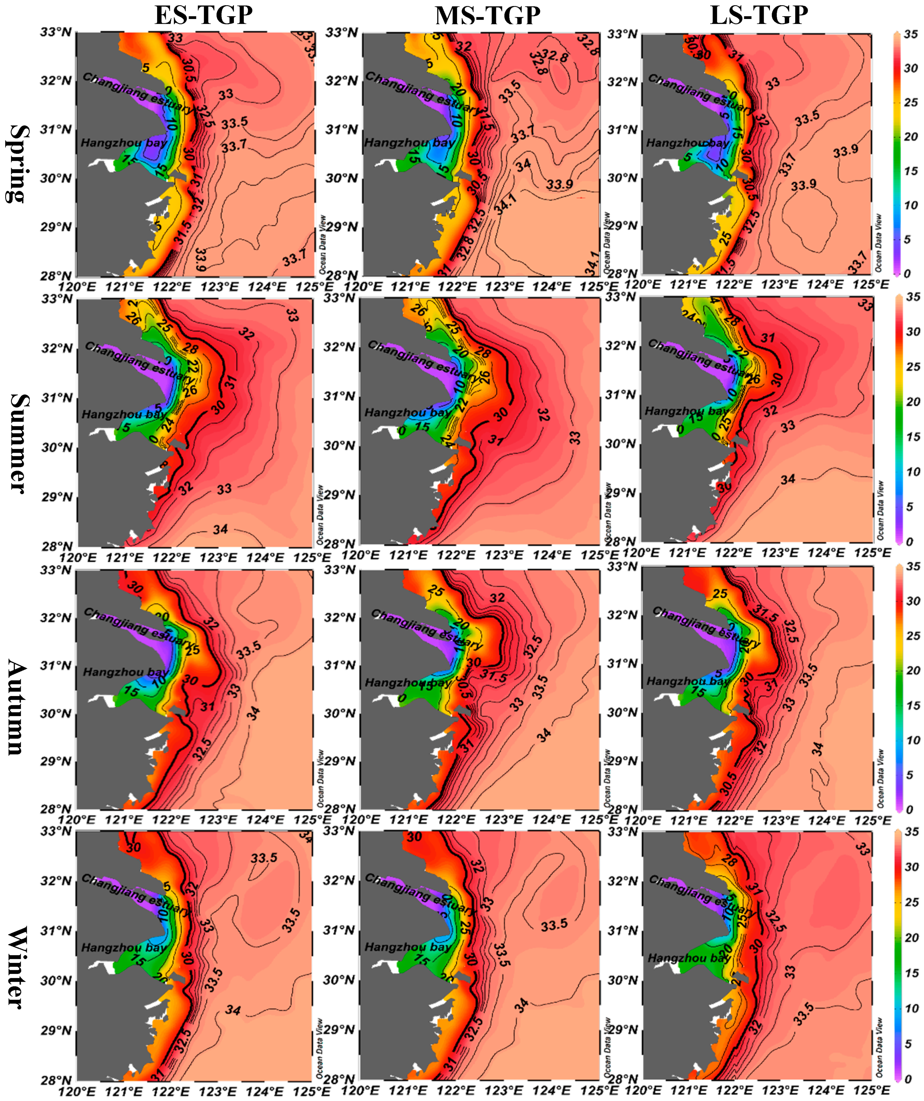
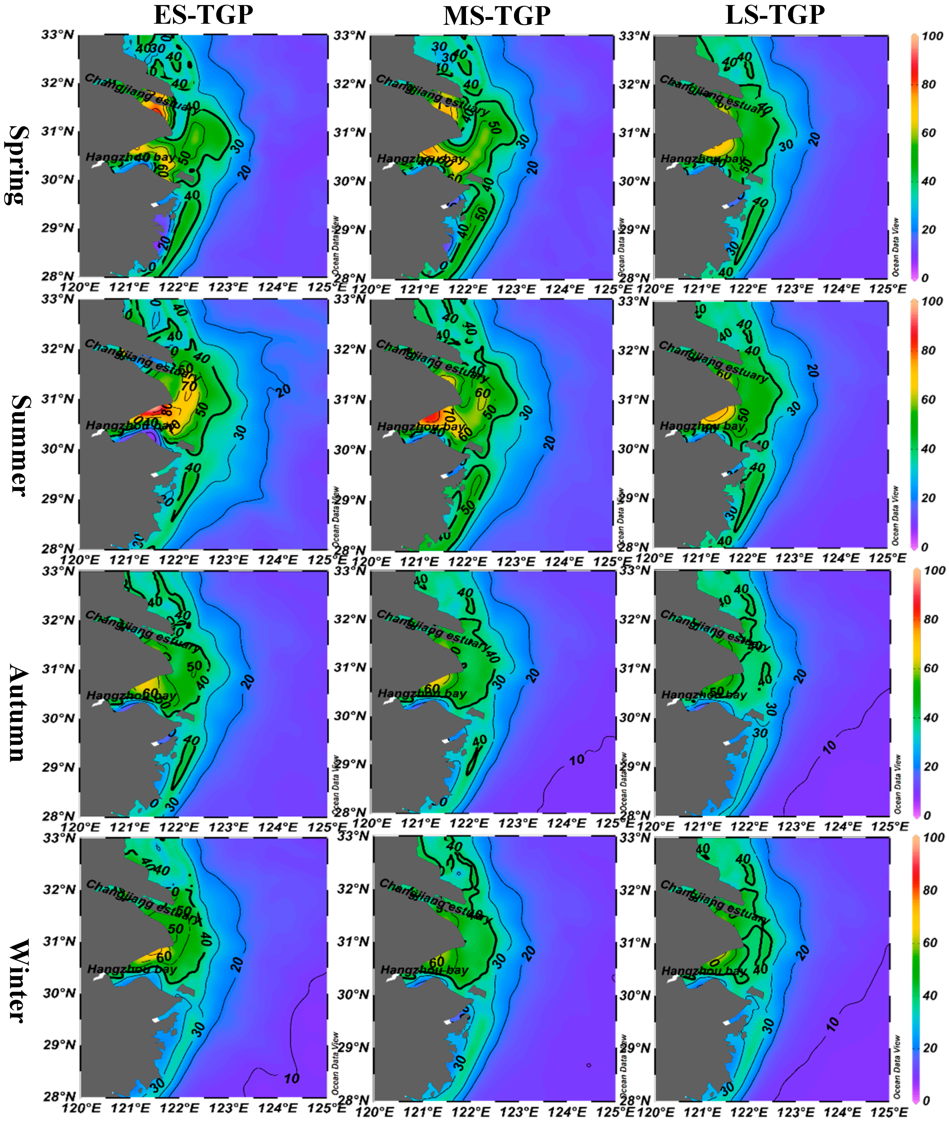
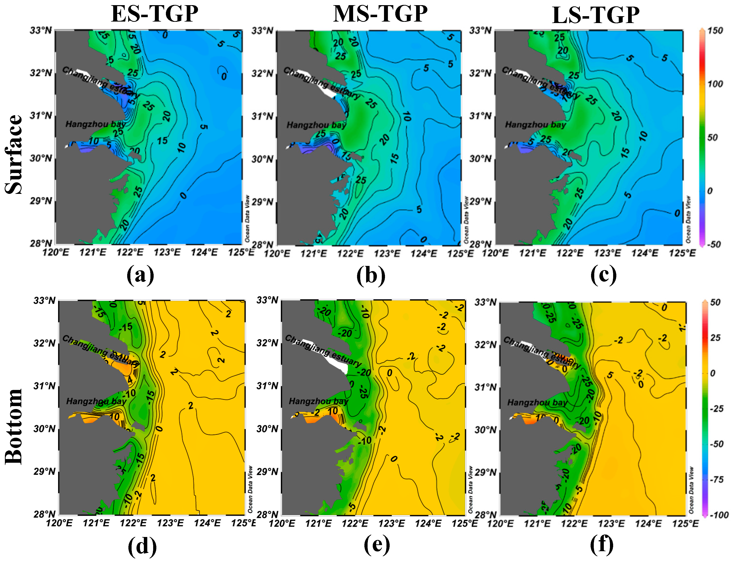
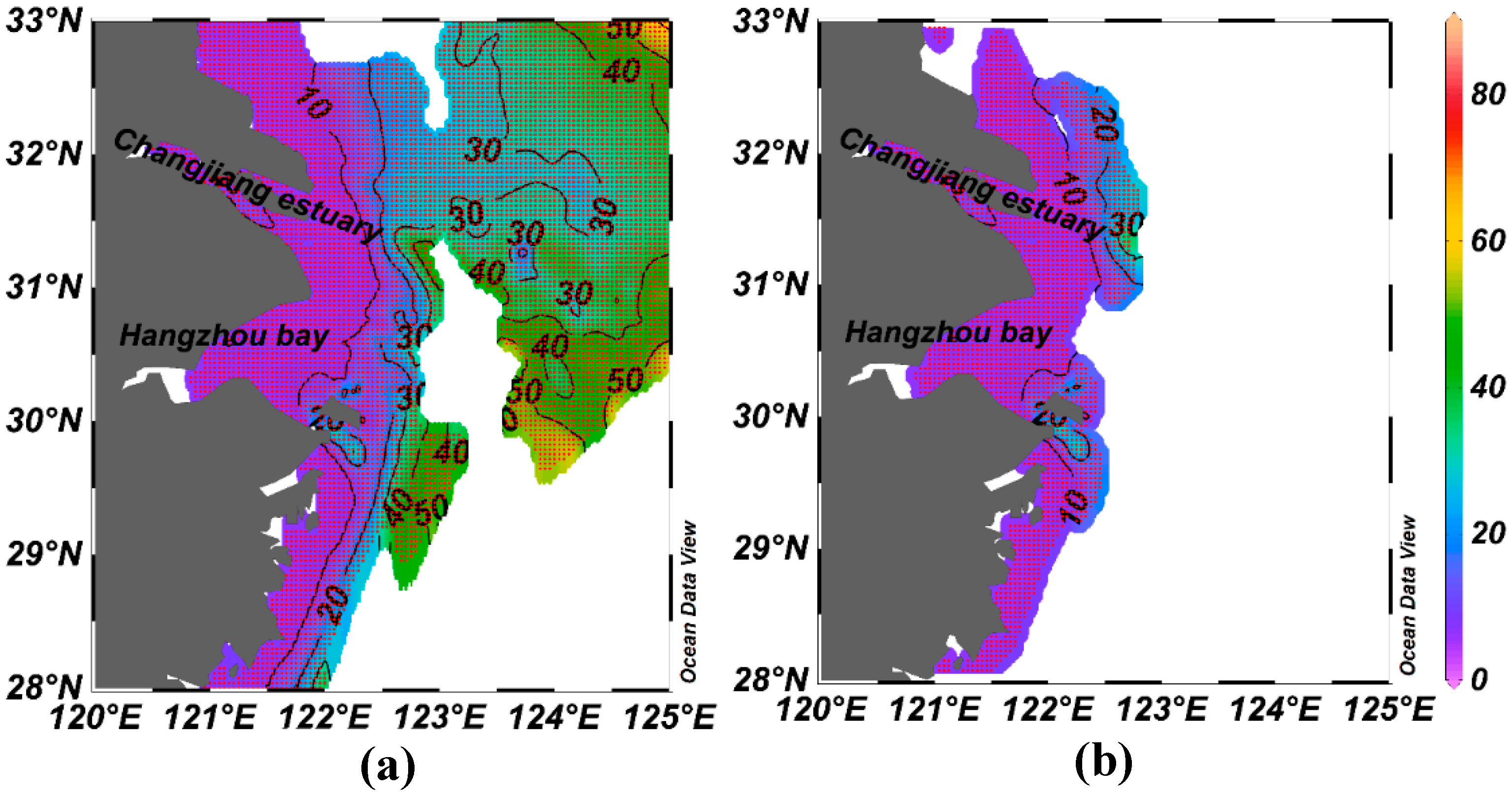
3.2. Seasonal Distribution
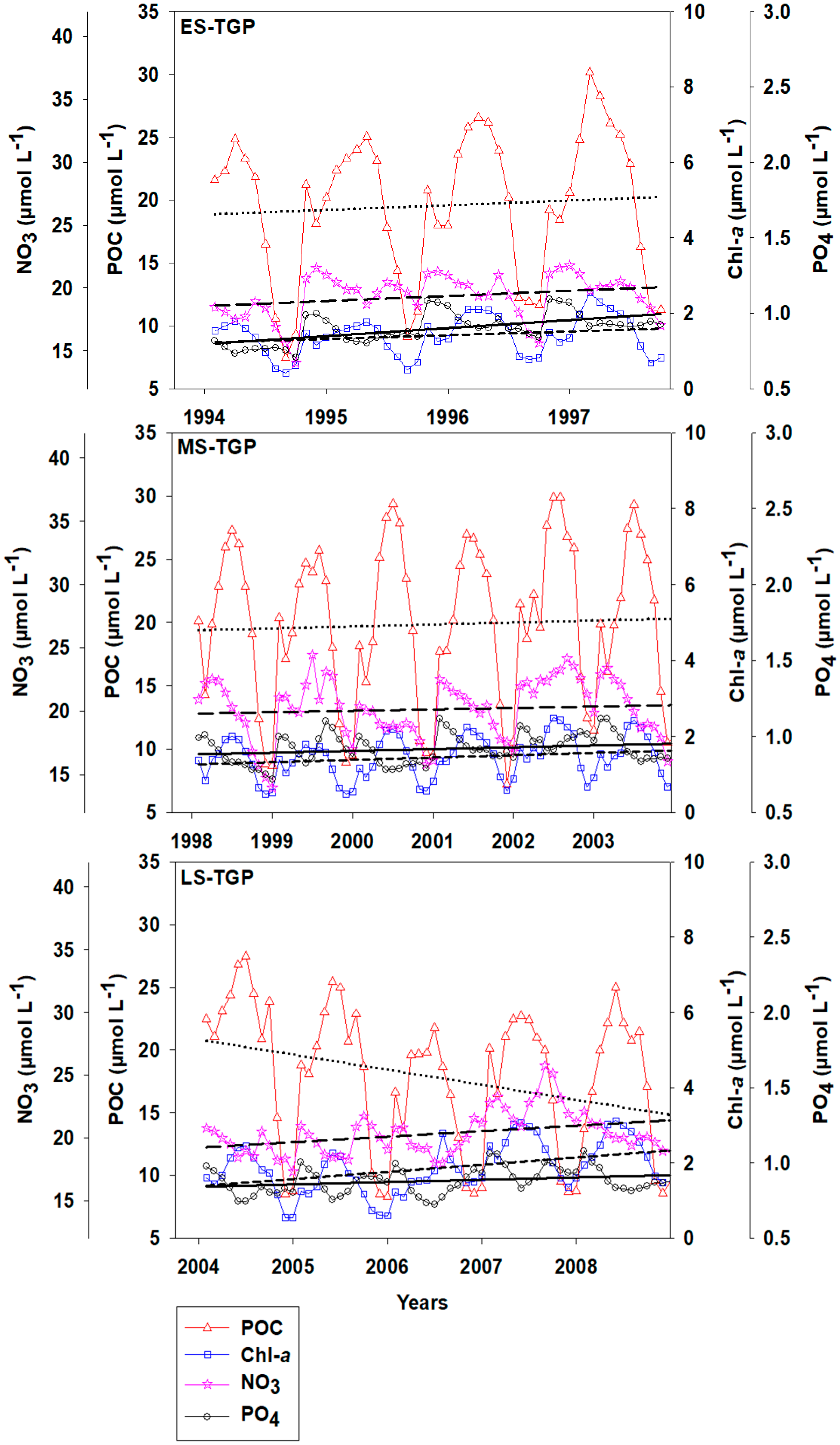
3.3. POC and Related Variables
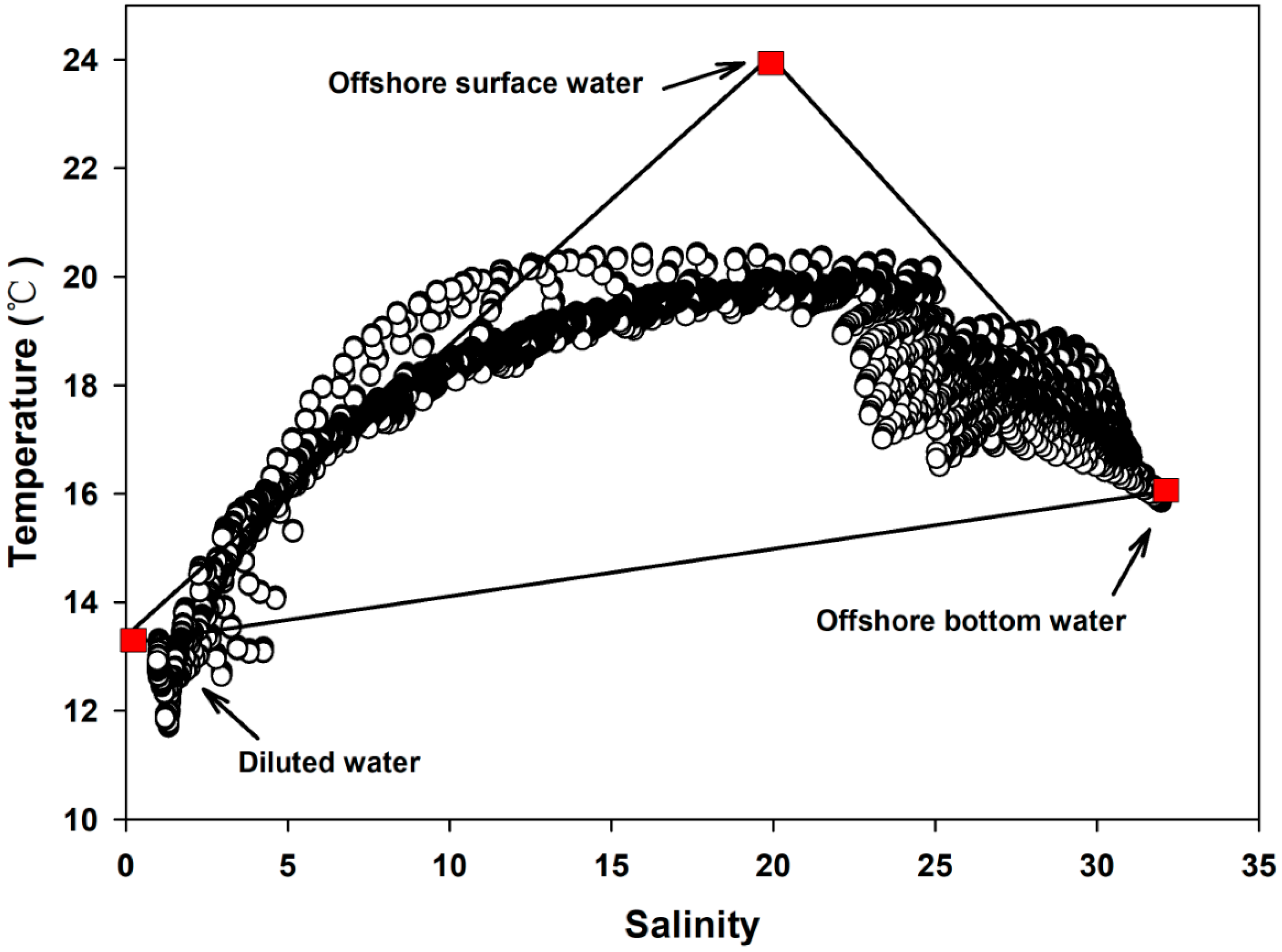
3.4. Three End-Member Mixing Model
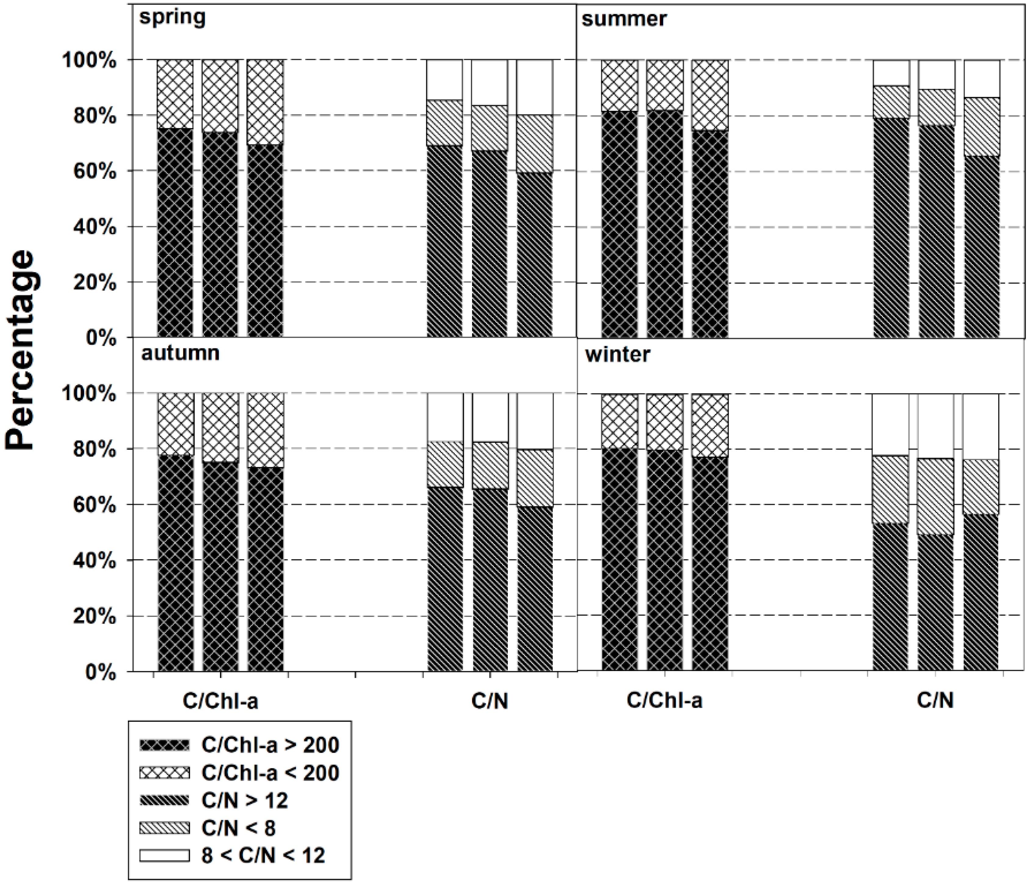
3.5. Ratio Variation
4. Conclusions
Author Contributions
Funding
Acknowledgments
Conflicts of Interest
References
- Nelson, D.; Sommers, L.E. Total carbon, organic carbon, and organic matter 1. In Methods of Soil Analysis, Part 2. Chemical and Microbiological Properties; American Society of Agronomy: Madison, WI, USA, 1982; pp. 539–579. [Google Scholar]
- Jahnke, R.A. The global ocean flux of particulate organic carbon: Areal distribution and magnitude. Glob. Biogeochem. Cycles 1996, 10, 71–88. [Google Scholar] [CrossRef]
- Suess, E. Particulate organic carbon flux in the oceans—Surface productivity and oxygen utilization. Nature 1980, 288, 260. [Google Scholar] [CrossRef]
- Armstrong, R.A.; Lee, C.; Hedges, J.I.; Honjo, S.; Wakeham, S.G. A new, mechanistic model for organic carbon fluxes in the ocean based on the quantitative association of POC with ballast minerals. Deep Sea Res. Part II Top. Stud. Oceanogr. 2001, 49, 219–236. [Google Scholar] [CrossRef]
- Lutz, M.J.; Caldeira, K.; Dunbar, R.B.; Behrenfeld, M.J. Seasonal rhythms of net primary production and particulate organic carbon flux to depth describe the efficiency of biological pump in the global ocean. J. Geophys. Res. Ocean. 2007, 112. [Google Scholar] [CrossRef]
- Turner, J.T. Zooplankton fecal pellets, marine snow, phytodetritus and the ocean’s biological pump. Prog. Oceanogr. 2015, 130, 205–248. [Google Scholar] [CrossRef]
- Schlünz, B.; Schneider, R. Transport of terrestrial organic carbon to the oceans by rivers: Re-estimating flux-and burial rates. Int. J. Earth Sci. 2000, 88, 599–606. [Google Scholar] [CrossRef]
- Spilling, K.; Kremp, A.; Klais, R.; Olli, K.; Tamminen, T. Spring bloom community change modifies carbon pathways and C: N: P: Chl a stoichiometry of coastal material fluxes. Biogeosciences 2014, 11, 7275–7289. [Google Scholar] [CrossRef]
- Sarà, G.; Leonardi, M.; Mazzola, A. Spatial and temporal changes of suspended matter in relation to wind and vegetation cover in a Mediterranean shallow coastal environment. Chem. Ecol. 1999, 16, 151–173. [Google Scholar] [CrossRef]
- Haskell, W.Z., II; Kadko, D.; Hammond, D.E.; Knapp, A.N.; Prokopenko, M.G.; Berelson, W.M.; Capone, D.G. Upwelling velocity and eddy diffusivity from 7Be measurements used to compare vertical nutrient flux to export POC flux in the Eastern Tropical South Pacific. Mar. Chem. 2015, 168, 140–150. [Google Scholar] [CrossRef]
- Hill, J.; Wheeler, P. Organic carbon and nitrogen in the northern California current system: Comparison of offshore, river plume, and coastally upwelled waters. Prog. Oceanogr. 2002, 53, 369–387. [Google Scholar] [CrossRef]
- Gao, L.; Li, D.; Zhang, Y. Nutrients and particulate organic matter discharged by the Changjiang (Yangtze River): Seasonal variations and temporal trends. J. Geophys. Res. Biogeosci 2012, 117. [Google Scholar] [CrossRef] [Green Version]
- Grossmann, M.M.; Gallager, S.M.; Mitarai, S. Continuous monitoring of near-bottom mesoplankton communities in the East China Sea during a series of typhoons. J. Oceanogr. 2015, 71, 115–124. [Google Scholar] [CrossRef]
- Vidon, P.; Karwan, D.L.; Andres, A.S.; Inamdar, S.; Kaushal, S.; Morrison, J.; Mullaney, J.; Ross, D.S.; Schroth, A.W.; Shanley, J.B. In the path of the Hurricane: Impact of Hurricane Irene and Tropical Storm Lee on watershed hydrology and biogeochemistry from North Carolina to Maine, USA. Biogeochemistry 2018, 141, 351–364. [Google Scholar] [CrossRef]
- Shih, Y.-Y.; Jin-Sheng, H.; Gong, G.-C.; Chin-Chang, H.; Wen-Chen, C.; Ming-An, L.; Kuo-Shu, C.; Meng-Hsien, C.; Chau-Ron, W. Field observations of changes in SST, chlorophyll and POC flux in the southern East China Sea before and after the passage of Typhoon Jangmi. TAO Terr. Atmos. Ocean. Sci. 2013, 24, 899. [Google Scholar] [CrossRef]
- Chen, D.; He, L.; Liu, F.; Yin, K. Effects of typhoon events on chlorophyll and carbon fixation in different regions of the East China Sea. Estuar. Coast. Shelf Sci. 2017, 194, 229–239. [Google Scholar] [CrossRef]
- Yang, Z.-S.; Wang, H.-J.; Saito, Y.; Milliman, J.; Xu, K.; Qiao, S.; Shi, G. Dam impacts on the Changjiang (Yangtze) River sediment discharge to the sea: The past 55 years and after the Three Gorges Dam. Water Resour. Res. 2006, 42. [Google Scholar] [CrossRef]
- Dai, Z.; Du, J.; Li, J.; Li, W.; Chen, J. Runoff characteristics of the Changjiang River during 2006: Effect of extreme drought and the impounding of the Three Gorges Dam. Geophys. Res. Lett. 2008, 35. [Google Scholar] [CrossRef]
- Liu, W. Study on particulate organic carbon in the East China Sea. Oceanol. Limnol. Sin. 1997, 28, 39–43. [Google Scholar]
- Chen, C.T.A. The Three Gorges Dam: Reducing the upwelling and thus productivity in the East China Sea. Geophys. Res. Lett. 2000, 27, 381–383. [Google Scholar] [CrossRef]
- Jiao, N.; Zhang, Y.; Zeng, Y.; Gardner, W.D.; Mishonov, A.V.; Richardson, M.J.; Hong, N.; Pan, D.; Yan, X.-H.; Jo, Y.-H. Ecological anomalies in the East China Sea: Impacts of the three gorges dam? Water Res. 2007, 41, 1287–1293. [Google Scholar] [CrossRef] [PubMed]
- Chen, X.; Yan, Y.; Fu, R.; Dou, X.; Zhang, E. Sediment transport from the Yangtze River, China, into the sea over the Post-Three Gorge Dam Period: A discussion. Quat. Int. 2008, 186, 55–64. [Google Scholar] [CrossRef]
- Dai, Z.; Du, J.; Zhang, X.; Su, N.; Li, J. Variation of riverine material loads and environmental consequences on the Changjiang (Yangtze) Estuary in recent decades (1955–2008). Environ. Sci. Technol. 2010, 45, 223–227. [Google Scholar] [CrossRef] [PubMed]
- Yang, S.; Milliman, J.; Li, P.; Xu, K. 50,000 dams later: Erosion of the Yangtze River and its delta. Glob. Planet. Chang. 2011, 75, 14–20. [Google Scholar] [CrossRef]
- Xu, K.; Milliman, J.D. Seasonal variations of sediment discharge from the Yangtze River before and after impoundment of the Three Gorges Dam. Geomorphology 2009, 104, 276–283. [Google Scholar] [CrossRef]
- Tang, Q.; Bao, Y.; He, X.; Fu, B.; Collins, A.L.; Zhang, X. Flow regulation manipulates contemporary seasonal sedimentary dynamics in the reservoir fluctuation zone of the Three Gorges Reservoir, China. Sci. Total Environ. 2016, 548, 410–420. [Google Scholar] [CrossRef] [PubMed]
- Chen, C.T.A.; Wang, S.L. Carbon, alkalinity and nutrient budgets on the East China Sea continental shelf. J. Geophys. Res. Ocean. 1999, 104, 20675–20686. [Google Scholar] [CrossRef]
- Zhou, F.; Chai, F.; Huang, D.; Xue, H.; Chen, J.; Xiu, P.; Xuan, J.; Li, J.; Zeng, D.; Ni, X. Investigation of hypoxia off the Changjiang Estuary using a coupled model of ROMS-CoSiNE. Prog. Oceanogr. 2017, 159, 237–254. [Google Scholar] [CrossRef]
- Luo, X.; Wei, H.; Liu, Z.; Zhao, L. Seasonal variability of air-sea CO2 fluxes in the Yellow and East China Seas: A case study of continental shelf sea carbon cycle model. Cont. Shelf Res. 2015, 107, 69–78. [Google Scholar] [CrossRef]
- Watanabe, K.; Kuwae, T. How organic carbon derived from multiple sources contributes to carbon sequestration processes in a shallow coastal system? Glob. Chang. Biol. 2015, 21, 2612–2623. [Google Scholar]
- Yamaguchi, H.; Kim, H.-C.; Son, Y.B.; Kim, S.W.; Okamura, K.; Kiyomoto, Y.; Ishizaka, J. Seasonal and summer interannual variations of SeaWiFS chlorophyll a in the Yellow Sea and East China Sea. Prog. Oceanogr. 2012, 105, 22–29. [Google Scholar] [CrossRef]
- Chai, F.; Dugdale, R.; Peng, T.-H.; Wilkerson, F.; Barber, R. One-dimensional ecosystem model of the equatorial Pacific upwelling system. Part I: Model development and silicon and nitrogen cycle. Deep Sea Res. Part II Top. Stud. Oceanogr. 2002, 49, 2713–2745. [Google Scholar] [CrossRef]
- Ezcurra, E.; Barrios, E.; Ezcurra, P.; Ezcurra, A.; Vanderplank, S.; Vidal, O.; Villanueva-Almanza, L.; Aburto-Oropeza, O. A natural experiment reveals the impact of hydroelectric dams on the estuaries of tropical rivers. Sci. Adv. 2019, 5, 9875. [Google Scholar] [CrossRef] [PubMed]
- Moore, A.M.; Arango, H.G.; Di Lorenzo, E.; Cornuelle, B.D.; Miller, A.J.; Neilson, D.J. A comprehensive ocean prediction and analysis system based on the tangent linear and adjoint of a regional ocean model. Ocean Model. 2004, 7, 227–258. [Google Scholar] [CrossRef]
- Shchepetkin, A.F.; McWilliams, J.C. The regional oceanic modeling system (ROMS): A split-explicit, free-surface, topography-following-coordinate oceanic model. Ocean Model. 2005, 9, 347–404. [Google Scholar] [CrossRef]
- Peliz, Á.; Dubert, J.; Haidvogel, D.B.; Le Cann, B. Generation and unstable evolution of a density-driven eastern poleward current: The Iberian Poleward Current. J. Geophys. Res. Ocean. 2003, 108. [Google Scholar] [CrossRef]
- Smith, R.N.; Chao, Y.; Li, P.P.; Caron, D.A.; Jones, B.H.; Sukhatme, G.S. Planning and implementing trajectories for autonomous underwater vehicles to track evolving ocean processes based on predictions from a regional ocean model. Int. J. Robot. Res. 2010, 29, 1475–1497. [Google Scholar] [CrossRef]
- Liu, Q.; Rothstein, L.M.; Luo, Y. Dynamics of the Block Island Sound estuarine plume. J. Phys. Oceanogr. 2016, 46, 1633–1656. [Google Scholar] [CrossRef]
- Liu, Q.; Rothstein, L.M.; Luo, Y. A periodic freshwater patch detachment process from the Block Island S ound estuarine plume. J. Geophys. Res. Ocean. 2017, 122, 570–586. [Google Scholar] [CrossRef]
- Zhou, F.; Xue, H.; Huang, D.; Xuan, J.; Ni, X.; Xiu, P.; Hao, Q. Cross-shelf exchange in the shelf of the East China Sea. J. Geophys. Res. Ocean. 2015, 120, 1545–1572. [Google Scholar] [CrossRef]
- Egbert, G.D.; Erofeeva, S.Y. Efficient inverse modeling of barotropic ocean tides. J. Atmos. Ocean. Technol. 2002, 19, 183–204. [Google Scholar] [CrossRef]
- Yangtze Statistical Yearbook 1994–2008; Yangtze River Statistical Publishing House: Wuhan, China, 2008.
- Chang, P.H.; Isobe, A. A numerical study on the Changjiang diluted water in the Yellow and East China Seas. J. Geophys. Res. Ocean. 2003, 108. [Google Scholar] [CrossRef]
- Large, W.; Pond, S. Open ocean momentum flux measurements in moderate to strong winds. J. Phys. Oceanogr. 1981, 11, 324–336. [Google Scholar] [CrossRef]
- Kalnay, E.; Kanamitsu, M.; Kistler, R.; Collins, W.; Deaven, D.; Gandin, L.; Iredell, M.; Saha, S.; White, G.; Woollen, J. The NCEP/NCAR 40-year reanalysis project. Bull. Am. Meteorol. Soc. 1996, 77, 437–472. [Google Scholar] [CrossRef]
- Zhang, H.M.; Bates, J.J.; Reynolds, R.W. Assessment of composite global sampling: Sea surface wind speed. Geophys. Res. Lett. 2006, 33. [Google Scholar] [CrossRef]
- Liu, Q.; Chai, F.; Dugdale, R.; Chao, Y.; Xue, H.; Rao, S.; Wilkerson, F.; Farrara, J.; Zhang, H.; Wang, Z. San Francisco Bay nutrients and plankton dynamics as simulated by a coupled hydrodynamic-ecosystem model. Cont. Shelf Res. 2018, 161, 29–48. [Google Scholar] [CrossRef]
- Chavez, F.P.; Buck, K.R.; Coale, K.; Martin, J.; DiTullio, G.; Welschmeyer, N.; Jacobson, A.C.; Barber, R.T. Growth rates, grazing, sinking, and iron limitation of equatorial Pacific phytoplankton. Limnol. Oceanogr. 1991, 36, 1816–1833. [Google Scholar] [CrossRef]
- Landry, M.R.; Constantinou, J.; Kirshtein, J. Microzooplankton grazing in the central equatorial Pacific during February and August, 1992. Deep Sea Res. Part II Top. Stud. Oceanogr. 1995, 42, 657–671. [Google Scholar] [CrossRef]
- Coale, K.H.; Johnson, K.S.; Fitzwater, S.E.; Gordon, R.M.; Tanner, S.; Chavez, F.P.; Ferioli, L.; Sakamoto, C.; Rogers, P.; Millero, F. A massive phytoplankton bloom induced by an ecosystem-scale iron fertilization experiment in the equatorial Pacific Ocean. Nature 1996, 383, 495. [Google Scholar] [CrossRef] [PubMed]
- Frost, B.; Franzen, N. Grazing and iron limitation in the control of phytoplankton stock and nutrient concentration: A chemostat analogue of the Pacific equatorial upwelling zone. Mar. Ecol. Prog. Ser. Oldend. 1992, 83, 291–303. [Google Scholar] [CrossRef]
- Anderson, L.A.; Sarmiento, J.L. Redfield ratios of remineralization determined by nutrient data analysis. Glob. Biogeochem. Cycles 1994, 8, 65–80. [Google Scholar] [CrossRef]
- Redfeild, A. The influence of organisms on the composition of sea water. Sea 1963, 2, 26–77. [Google Scholar]
- Xiu, P.; Chai, F. Spatial and temporal variability in phytoplankton carbon, chlorophyll, and nitrogen in the North Pacific. J. Geophys. Res. Ocean. 2012, 117. [Google Scholar] [CrossRef]
- Ludwig, W.; Probst, J.L.; Kempe, S. Predicting the oceanic input of organic carbon by continental erosion. Glob. Biogeochem. Cycles 1996, 10, 23–41. [Google Scholar] [CrossRef] [Green Version]
- River Sediment Bulletin of China 1994–2008; China Water & Power Press: Beijing, China, 2008.
- Xiu, P.; Chai, F. Modeled biogeochemical responses to mesoscale eddies in the South China Sea. J. Geophys. Res. Ocean. 2011, 116. [Google Scholar] [CrossRef] [Green Version]
- Isobe, A.; Guo, X.; Takeoka, H. Hindcast and predictability of sporadic Kuroshio-water intrusion (kyucho in the Bungo Channel) into the shelf and coastal waters. J. Geophys. Res. Ocean. 2010, 115. [Google Scholar] [CrossRef]
- Kunoki, S.; Manda, A.; Kodama, Y.; Iizuka, S.; Sato, K.; Fathrio, I.; Mitsui, T.; Seko, H.; Moteki, Q.; Minobe, S. Oceanic influence on the Baiu frontal zone in the East China Sea. J. Geophys. Res. 2015, 120, 449–463. [Google Scholar] [CrossRef]
- Iseki, K.; Okamura, K.; Kiyomoto, Y. Seasonality and composition of downward particulate fluxes at the continental shelf and Okinawa Trough in the East China Sea. Deep Sea Res. Part II Top. Stud. Oceanogr. 2003, 50, 457–473. [Google Scholar] [CrossRef]
- Zhao, J.-S.; Ji, H.-W.; Guo, Z.-G. The vertical distribution of particulate organic carbon in the typical areas of the East China Sea in winter. Mar. Sci. Qingdao Chin. Ed. 2003, 27, 59–63. [Google Scholar]
- Zhu, Z.Y.; Zhang, J.; Wu, Y.; Lin, J. Bulk particulate organic carbon in the East China Sea: Tidal influence and bottom transport. Prog. Oceanogr. 2006, 69, 37–60. [Google Scholar] [CrossRef]
- Song, X.-H.; Shi, X.-F.; Cai, D.-L.; Wang, G.-Q.; Wang, J.-T. Distributions of TSM, POC and PN in the Changjiang Estuary area in autumn after the river closure at Three Gorges. Adv. Mar. Sci. 2007, 25, 168. [Google Scholar]
- Shi, X.; Zhang, T.; Zhang, C.; Cheng, J. Spatial and temporal distribution of particulate organic carbon in Yellow Sea and East China Sea. Mar. Environ. Sci. 2011, 1, 25–29. [Google Scholar]
- Hung, C.-C.; Tseng, C.-W.; Gong, G.-C.; Chen, K.-S.; Chen, M.-H.; Hsu, S.-C. Fluxes of particulate organic carbon in the East China Sea in summer. Biogeosciences 2013, 10, 6469–6484. [Google Scholar] [CrossRef] [Green Version]
- Pan, J.W.; Zhu, J. Scientific Verification is the Basis for Correct Decision-making of Major Project—Practical Proof on Verification Conclusions of TGP. Eng. Sci. 2001, 3, 21–26. [Google Scholar]
- Jiazhu, W. Three Gorges Project: The largest water conservancy project in the world. Public Adm. Dev. Int. J. Manag. Res. Pract. 2002, 22, 369–375. [Google Scholar] [CrossRef]
- Lau, K.; Weng, H. Coherent modes of global SST and summer rainfall over China: An assessment of the regional impacts of the 1997–1998 El Nino. J. Clim. 2001, 14, 1294–1308. [Google Scholar] [CrossRef]
- Dai, Z.; Fagherazzi, S.; Mei, X.; Gao, J. Decline in suspended sediment concentration delivered by the Changjiang (Yangtze) River into the East China Sea between 1956 and 2013. Geomorphology 2016, 268, 123–132. [Google Scholar] [CrossRef] [Green Version]
- Dai, Z.; Liu, J.T. Impacts of large dams on downstream fluvial sedimentation: An example of the Three Gorges Dam (TGD) on the Changjiang (Yangtze River). J. Hydrol. 2013, 480, 10–18. [Google Scholar] [CrossRef]
- Zhang, W.; Xu, Y.; Wang, Y.; Peng, H. Modeling sediment transport and river bed evolution in river system. J. Clean Energy Technol. 2014, 2, 175–179. [Google Scholar] [CrossRef]
- Milliman, J.D.; Qinchun, X.; Zuosheng, Y. Transfer of particulate organic carbon and nitrogen from the Yangtze River to the ocean. Am. J. Sci. 1984, 284, 824–834. [Google Scholar] [CrossRef]
- Gao, X.; Song, J. Phytoplankton distributions and their relationship with the environment in the Changjiang Estuary, China. Mar. Pollut. Bull. 2005, 50, 327–335. [Google Scholar] [CrossRef]
- Shi, J.Z.; Zhang, S.; Hamilton, L. Bottom fine sediment boundary layer and transport processes at the mouth of the Changjiang Estuary, China. J. Hydrol. 2006, 327, 276–288. [Google Scholar] [CrossRef]
- Li, D.; Zhang, J.; Huang, D.; Wu, Y.; Liang, J. Oxygen depletion off the Changjiang (Yangtze River) estuary. Sci. China Ser. D Earth Sci. 2002, 45, 1137–1146. [Google Scholar] [CrossRef]
- Chen, C.; Xue, P.; Ding, P.; Beardsley, R.C.; Xu, Q.; Mao, X.; Gao, G.; Qi, J.; Li, C.; Lin, H. Physical mechanisms for the offshore detachment of the Changjiang Diluted Water in the East China Sea. J. Geophys. Res. Ocean. 2008, 113. [Google Scholar] [CrossRef]
- Zhu, J.; Zhu, Z.; Lin, J.; Wu, H.; Zhang, J. Distribution of hypoxia and pycnocline off the Changjiang Estuary, China. J. Mar. Syst. 2016, 154, 28–40. [Google Scholar] [CrossRef]
- Gao, X.; Song, J. Main geochemical characteristics and key biogeochemical carbon processes in the East China Sea. J. Coast. Res. 2006, 22, 1330–1339. [Google Scholar] [CrossRef]
- Hung, C.-C.; Gong, G.-C.; Chiang, K.-P.; Chen, H.-Y.; Yeager, K.M. Particulate carbohydrates and uronic acids in the northern East China Sea. Estuar. Coast. Shelf Sci. 2009, 84, 565–572. [Google Scholar] [CrossRef]
- Van Mooy, B.A.; Fredricks, H.F.; Pedler, B.E.; Dyhrman, S.T.; Karl, D.M.; Koblížek, M.; Lomas, M.W.; Mincer, T.J.; Moore, L.R.; Moutin, T. Phytoplankton in the ocean use non-phosphorus lipids in response to phosphorus scarcity. Nature 2009, 458, 69. [Google Scholar] [CrossRef]
- Hu, J.; Yang, S.-F.; Wang, X.-K. Sedimentation in Yangtze River above Three Gorges Project since 2003. J. Sediment. Res. 2013, 1, 39–40. [Google Scholar]
- Yang, S.; Belkin, I.; Belkina, A.; Zhao, Q.; Zhu, J.; Ding, P. Delta response to decline in sediment supply from the Yangtze River: Evidence of the recent four decades and expectations for the next half-century. Estuar. Coast. Sci. 2003, 57, 689–699. [Google Scholar] [CrossRef]
- Li, P.; Yang, S.; Milliman, J.; Xu, K.; Qin, W.; Wu, C.; Chen, Y.; Shi, B. Spatial, temporal, and human-induced variations in suspended sediment concentration in the surface waters of the Yangtze Estuary and adjacent coastal areas. Estuaries Coasts 2012, 35, 1316–1327. [Google Scholar] [CrossRef]
- Luo, X.; Yang, S.; Zhang, J. The impact of the Three Gorges Dam on the downstream distribution and texture of sediments along the middle and lower Yangtze River (Changjiang) and its estuary, and subsequent sediment dispersal in the East China Sea. Geomorphology 2012, 179, 126–140. [Google Scholar] [CrossRef]
- Keeling, R.F.; Peng, T.-H. Transport of heat, CO2 and O2 by the Atlantic’s thermohaline circulation. Philos. Trans. R. Soc. Lond. Ser. B Biol. Sci. 1995, 348, 133–142. [Google Scholar]
- Han, A.; Dai, M.; Kao, S.-J.; Gan, J.; Li, Q.; Wang, L.; Zhai, W.; Wang, L. Nutrient dynamics and biological consumption in a large continental shelf system under the influence of both a river plume and coastal upwelling. Limnol. Oceanogr. 2012, 57, 486–502. [Google Scholar] [CrossRef] [Green Version]
- Wang, K.; Chen, J.; Jin, H.; Li, H.; Gao, S.; Xu, J.; Lu, Y.; Huang, D.; Hao, Q.; Weng, H. Summer nutrient dynamics and biological carbon uptake rate in the Changjiang River plume inferred using a three end-member mixing model. Cont. Shelf Res. 2014, 91, 192–200. [Google Scholar] [CrossRef]
- Li, D.; Yao, P.; Bianchi, T.S.; Zhang, T.; Zhao, B.; Pan, H.; Wang, J.; Yu, Z. Organic carbon cycling in sediments of the Changjiang Estuary and adjacent shelf: Implication for the influence of Three Gorges Dam. J. Mar. Syst. 2014, 139, 409–419. [Google Scholar] [CrossRef]
- Dickson, B.; Yashayaev, I.; Meincke, J.; Turrell, B.; Dye, S.; Holfort, J. Rapid freshening of the deep North Atlantic Ocean over the past four decades. Nature 2002, 416, 832. [Google Scholar] [CrossRef] [PubMed]
- Yu-song, S.; Xue-chuan, W. Water masses in China seas. In Oceanology of China Seas; Springer: Berlin, Germany, 1994; pp. 3–16. [Google Scholar]
- Wei, H.; He, Y.; Li, Q.; Liu, Z.; Wang, H. Summer hypoxia adjacent to the Changjiang Estuary. J. Mar. Syst. 2007, 67, 292–303. [Google Scholar] [CrossRef]
- Beardsley, R.; Limeburner, R.; Yu, H.; Cannon, G. Discharge of the Changjiang (Yangtze river) into the East China sea. Cont. Shelf Res. 1985, 4, 57–76. [Google Scholar] [CrossRef]
- Zhai, W.D.; Chen, J.F.; Jin, H.Y.; Li, H.L.; Liu, J.W.; He, X.Q.; Bai, Y. Spring carbonate chemistry dynamics of surface waters in the northern East China Sea: Water mixing, biological uptake of CO2, and chemical buffering capacity. J. Geophys. Res. Ocean. 2014, 119, 5638–5653. [Google Scholar] [CrossRef]
- Li, P.; Shi, B.; Wang, Y.; Qin, W.; Li, Y.; Chen, J. Analysis of the characteristics of offshore currents in the Changjiang (Yangtze River) estuarine waters based on buoy observations. Acta Oceanol. Sin. 2017, 36, 13–20. [Google Scholar] [CrossRef]
- Zhang, J.; Liu, S.; Ren, J.; Wu, Y.; Zhang, G. Nutrient gradients from the eutrophic Changjiang (Yangtze River) Estuary to the oligotrophic Kuroshio waters and re-evaluation of budgets for the East China Sea Shelf. Prog. Oceanogr. 2007, 74, 449–478. [Google Scholar] [CrossRef]
- Omand, M.M.; D’Asaro, E.A.; Lee, C.M.; Perry, M.J.; Briggs, N.; Cetinić, I.; Mahadevan, A. Eddy-driven subduction exports particulate organic carbon from the spring bloom. Science 2015, 348, 222–225. [Google Scholar] [CrossRef] [PubMed] [Green Version]
- Lian, E.; Yang, S.; Wu, H.; Yang, C.; Li, C.; Liu, J.T. Kuroshio subsurface water feeds the wintertime Taiwan Warm Current on the inner East China Sea shelf. J. Geophys. Res. Ocean. 2016, 121, 4790–4803. [Google Scholar] [CrossRef]
- Wu, H.; Zhu, J.; Shen, J.; Wang, H. Tidal modulation on the Changjiang River plume in summer. J. Geophys. Res. Ocean. 2011, 116. [Google Scholar] [CrossRef] [Green Version]
- Li, M.; Xu, K.; Watanabe, M.; Chen, Z. Long-term variations in dissolved silicate, nitrogen, and phosphorus flux from the Yangtze River into the East China Sea and impacts on estuarine ecosystem. Estuar. Coast. Shelf Sci. 2007, 71, 3–12. [Google Scholar] [CrossRef]
- Guo, H.; Hu, Q.; Zhang, Q.; Feng, S. Effects of the three gorges dam on Yangtze river flow and river interaction with Poyang Lake, China: 2003–2008. J. Hydrol. 2012, 416, 19–27. [Google Scholar] [CrossRef]
- Trefry, J.H.; Metz, S.; Nelsen, T.A.; Trocine, R.P.; Eadie, B.J. Transport of particulate organic carbon by the Mississippi River and its fate in the Gulf of Mexico. Estuaries 1994, 17, 839. [Google Scholar] [CrossRef]
- Liénart, C.; Susperregui, N.; Rouaud, V.; Cavalheiro, J.; David, V.; Del Amo, Y.; Duran, R.; Lauga, B.; Monperrus, M.; Pigot, T. Dynamics of particulate organic matter in a coastal system characterized by the occurrence of marine mucilage—A stable isotope study. J. Sea Res. 2016, 116, 12–22. [Google Scholar] [CrossRef]
- Hedges, J.; Keil, R.; Benner, R. What happens to terrestrial organic matter in the ocean? Org. Geochem. 1997, 27, 195–212. [Google Scholar] [CrossRef]
- Cai, W. Estuarine and Coastal Ocean Carbon Paradox: CO2 Sinks or Sites of Terrestrial Carbon Incineration? Annu. Rev. Mar. Sci. 2011, 3, 123–145. [Google Scholar] [CrossRef]
- Saliot, A.; Parrish, C.C.; Sadouni, N.m.; Bouloubassi, I.; Fillaux, J.; Cauwet, G. Transport and fate of Danube Delta terrestrial organic matter in the Northwest Black Sea mixing zone. Mar. Chem. 2002, 79, 243–259. [Google Scholar] [CrossRef]
- Gao, J.; Wang, Y.; Pan, S.; Zhang, R.; Li, J.; Bai, F. Spatial distributions of organic carbon and nitrogen and their isotopic compositions in sediments of the Changjiang Estuary and its adjacent sea area. J. Geogr. Sci. 2008, 18, 46–58. [Google Scholar] [CrossRef]
- Zhu, Z.-Y.; Ng, W.-M.; Liu, S.-M.; Zhang, J.; Chen, J.-C.; Wu, Y. Estuarine phytoplankton dynamics and shift of limiting factors: A study in the Changjiang (Yangtze River) Estuary and adjacent area. Estuar. Coast. Shelf Sci. 2009, 84, 393–401. [Google Scholar] [CrossRef]
- Ding, T.; Wan, D.; Wang, C.; Zhang, F. Silicon isotope compositions of dissolved silicon and suspended matter in the Yangtze River, China. Geochim. Cosmochim. Acta 2004, 68, 205–216. [Google Scholar] [CrossRef]
- Ma, N.; Li, Z.; Xia, S.; Zhu, Z.; Song, Z. Retention effects of river damming on dissolved silicon. Inland Waters 2018, 8, 207–215. [Google Scholar] [CrossRef]
- Jiang, Z.; Liu, J.; Chen, J.; Chen, Q.; Yan, X.; Xuan, J.; Zeng, J. Responses of summer phytoplankton community to drastic environmental changes in the Changjiang (Yangtze River) estuary during the past 50 years. Water Res. 2014, 54, 1–11. [Google Scholar] [CrossRef]
- Burkhardt, S.; Riebesell, U.; Zondervan, I. Effects of growth rate, CO2 concentration, and cell size on the stable carbon isotope fractionation in marine phytoplankton. Geochim. Cosmochim. Acta 1999, 63, 3729–3741. [Google Scholar] [CrossRef]
- Menden-Deuer, S.; Lessard, E.J. Carbon to volume relationships for dinoflagellates, diatoms, and other protist plankton. Limnol. Oceanogr. 2000, 45, 569–579. [Google Scholar] [CrossRef] [Green Version]


| Season Ends | t1/s1/p1 DW | t2/s2/p2 OSW | t3/s3/p3 OBW |
|---|---|---|---|
| Spring | 13.4/0.8/58.5 | 23.8/20.1/47.7 | 15.9/32.2/34.3 |
| Summer | 26.8/0.6/56.1 | 29.7/28.1/48.1 | 24.1/31.0/30.8 |
| Autumn | 20.9/0.6/49.9 | 24.2/28.3/42.4 | 19.5/31.6/31.5 |
| Winter | 10.3/0.9/42.8 | 16.6/29.5/33.8 | 12.4/32.2/28.9 |
| Period | Season | DW% | OBW% | OSW% |
|---|---|---|---|---|
| ES-TGP | Spring | 33.30% | 51.30% | 15.40% |
| Summer | 51.70% | 37.20% | 11.10% | |
| Autumn | 37.50% | 40.80% | 21.70% | |
| Winter | 26.30% | 60.40% | 13.30% | |
| MS-TGP | Spring | 33.80% | 43.80% | 22.40% |
| Summer | 56.20% | 31.50% | 12.30% | |
| Autumn | 38.60% | 42.50% | 18.90% | |
| Winter | 25.90% | 53.30% | 20.80% | |
| LS-TGP | Spring | 38.70% | 49.80% | 11.50% |
| Summer | 45.80% | 43.50% | 10.70% | |
| Autumn | 41.60% | 35.90% | 22.50% | |
| Winter | 34.90% | 40.00% | 25.10% |
© 2019 by the authors. Licensee MDPI, Basel, Switzerland. This article is an open access article distributed under the terms and conditions of the Creative Commons Attribution (CC BY) license (http://creativecommons.org/licenses/by/4.0/).
Share and Cite
Chen, D.; Liu, Q.; Xu, J.; Wang, K. Model-Based Evaluation of Hydroelectric Dam’s Impact on the Seasonal Variabilities of POC in Coastal Ocean: A Case Study of Three Gorges Project. J. Mar. Sci. Eng. 2019, 7, 320. https://doi.org/10.3390/jmse7090320
Chen D, Liu Q, Xu J, Wang K. Model-Based Evaluation of Hydroelectric Dam’s Impact on the Seasonal Variabilities of POC in Coastal Ocean: A Case Study of Three Gorges Project. Journal of Marine Science and Engineering. 2019; 7(9):320. https://doi.org/10.3390/jmse7090320
Chicago/Turabian StyleChen, Dongxing, Qianqian Liu, Jiexin Xu, and Kuo Wang. 2019. "Model-Based Evaluation of Hydroelectric Dam’s Impact on the Seasonal Variabilities of POC in Coastal Ocean: A Case Study of Three Gorges Project" Journal of Marine Science and Engineering 7, no. 9: 320. https://doi.org/10.3390/jmse7090320