Article

An Integrated Web-Based System for the Monitoring and Forecasting of Coastal Harmful Algae Blooms: Application to Shenzhen City, China

1
Guangdong Provincial Key Laboratory of Soil and Groundwater Pollution Control, School of Environmental Science and Engineering, Southern University of Science and Technology, Shenzhen 518055, China
2
Shenzhen Municipal Engineering Lab of Environmental IoT Technologies, Southern University of Science and Technology, Shenzhen 518055, China
3
School of Hydropower Engineering & Information Engineering, Huazhong University of Science & Technology, Wuhan 430074, China
*
Author to whom correspondence should be addressed.
J. Mar. Sci. Eng. 2019, 7(9), 314; https://doi.org/10.3390/jmse7090314
Submission received: 27 July 2019 / Revised: 28 August 2019 / Accepted: 6 September 2019 / Published: 9 September 2019

Abstract

:
Harmful algal blooms (HABs) cause environmental problems worldwide. Continuous monitoring and forecasting of harmful algal blooms are necessary for marine resources managers to detect the intensity and spatial extent of HABs and provide early warnings to the public. In this study, we introduce an integrated web-based system for the monitoring and forecasting of coastal HABs. The system is named the Harmful Algal Blooms Monitoring and Forecasting System (HMFS). HMFS integrates in situ observations, a remote-sensing-based model, hydrodynamic and water quality model and Web-Based Geographic Information System (GIS) techniques into one environment. The in situ sensors and remote sensing model provide automatic and continuous monitoring of the coastal water conditions. The numerical models provide short-term prediction and early warning of HAB of up to 5 days. The overall forecast accuracy is more than or equal to 50% for the major coastal areas of Shenzhen in 2018. By leveraging a web-based GIS technique and Service-Oriented Architecture (SOA), the web portal of HMFS provides a graphic interface for users and mangers to view real-time in situ measurements and remote sensing maps, explore numerical model forecasts and get early warning information. HMFS was applied to Shenzhen, which is a rising megacity in Southern China. The application study demonstrated the applicability and effectiveness of HMFS for monitoring and predicting HABs.

1. Introduction

The coastal and marine environment provides valuable natural resources for food, transportation, and recreation. It also hosts an invaluable biodiversity that forms complex ecosystems. Due to near-shore development, costal and marine ecosystems are being threatened by anthropogenic impacts including fisheries, aquaculture, shipping, urbanization and tourism, resulting in increased harmful algal blooms (HABs) events. HABs, also termed as red tides, generate toxic and harmful effects to the human body, fish, birds and marine ecosystem when present. In recent decades, HAB has been increased in frequency and spatial extent worldwide [1]. In China, HABs are a national concern because they have occurred in every coastal province and their occurrences are on the rise [2]. Shenzhen, one of the most developed areas in China, is also seriously affected by HAB occurrences. Algal blooms occurred more frequently in Shenzhen in recent decades [3,4], due to both natural and anthropogenic sources. Raid monitoring and accurate forecasting of HABs is an important task for local management agencies to protect marine resources.
A number of efforts have been made to detect the location and intensity of HABs and forecast the development of HABs. Detection of HABs strongly relies on in situ observations. Benefiting from the rapid development of real-time sensor technology and communication technology, many in situ monitoring systems have been developed to detect HABs by measuring marine water and environmental parameters in real-time. Remote sensing also plays an important role in detecting HABs. Several water column parameters can be monitored by satellites, such as chlorophyll-a (Chl-a) concentration, phytoplankton biomass, water transparency, and total suspended matter (TSM) concentrations. The data obtained from remote sensing of ocean properties is called ocean color data. Chl-a is usually used as a health indicator of the coastal and marine water. Many studies have been conducted to estimate Chl-a by using ocean color sensors, such as Sea-Viewing Wide Field-of-View Sensor (SeaWiFS) [5], the Medium-Resolution Imaging Spectrometer (MERIS) [6], and the Moderate-Resolution Imaging Spectroradiometer (MODIS) [7]. These sensors are specially designed for the assessment of ocean water quality parameters; However, their coarse spatial resolution (250~1000 m) limits their use in the coastal water regions. Landsat sensors, including Thematic Mapper (TM) [8], Enhanced Thematic Mapper Plus (ETM+) and Operational Land Imager (OLI) sensors, are designed for terrestrial applications, but they can also be used for studying coastal waters due to their high spatial resolution (30 m) [9,10].
Short-term forecasting of coastal HABs mainly relies on numerical models. Numerical modelling enables the prediction of occurrence timing, spatial extent and magnitude of a possible HAB event [11]. Many models and commercial software have been developed for numerical ocean modelling, including Finite-Volume Community Ocean Model (FVCOM) [12], MIKE3, Environmental Fluid Dynamics Code (EFDC), Princeton Ocean Model (POM), and Delft3D [13]. Despite the increasing accuracy of HABs forecasts, there is uncertainty in all predictions, resulting from inevitable uncertainties in the initial and boundary conditions and necessary approximations in the construction of a numerical model of the real ocean system. To reduce model uncertainties, data assimilation methods are increasingly used in ocean modeling. The core idea behind data assimilation is to integrate model dynamics and measured data, thereby providing a better simulation that is consistent with the observed fields [14]. The most widely used data assimilation techniques include nudging, optimal interpolation (OI) [15], Ensemble Kalman Filter (EnKF) [16], and Particle Filter [17].
Ocean observation data and modeling results are usually large-volume, multi-source, and multi-dimensional. It is usually difficult for end-users to understand, analyze and utilize these complex data sets. Bringing these data sets into one system and visualizing them in a geospatial context would greatly improve the understanding and management of HABs. Recent progress in Web-Based Geographic Information System (GIS) technologies provides a great opportunity to achieve this goal. A number of efforts have been made to develop online systems for coastal water management. For example, Kulawiak et al. introduce a Web-Based GIS system for monitoring and forecasting oil spill [18]. Qin and Lin developed a coastal seiches monitoring and forecasting system based on a Web-Based GIS platform [19]. Zhang et al. developed a system to forecast short-term algal bloom in Lake Taihu [20].
Despite the significant progress that has been made in monitoring techniques, numerical ocean modeling, remote sensing methods of ocean color and GIS, integrated systems that are capable of integrating these techniques and models into a single platform for HABs detection and forecasting are limited. This study introduces the design and development of a Web-Based GIS system named HABs Monitoring and Forecasting System (HMFS). The system is intended to rapidly detect and accurately predict coastal HABs events in Shenzhen city. HMFS integrates in situ observations, a remote-sensing-based model, hydrodynamic and water quality model and Web-Based GIS technique into one environment. The in situ sensors and remote sensing model provides continuous monitoring of the coastal water conditions. The numerical models provide short-term prediction and early warning of HAB. By leveraging a Web-Based GIS technique and Service-Oriented Architecture (SOA), the web portal of HMFS provides a graphic interface for users to view real-time data and remote sensing maps, explore numerical model outputs and get early warning information.
The remainder of this paper is organized as follows. Section 2 introduces the study area. Section 3 introduces the framework of the system, including system architecture and core system components. Section 4 describes the web portal of the system with the application case in Shenzhen. Conclusions are provided in Section 5.

2. Study Area

Shenzhen, a typical coastal city in China, covers an area of 1997 km
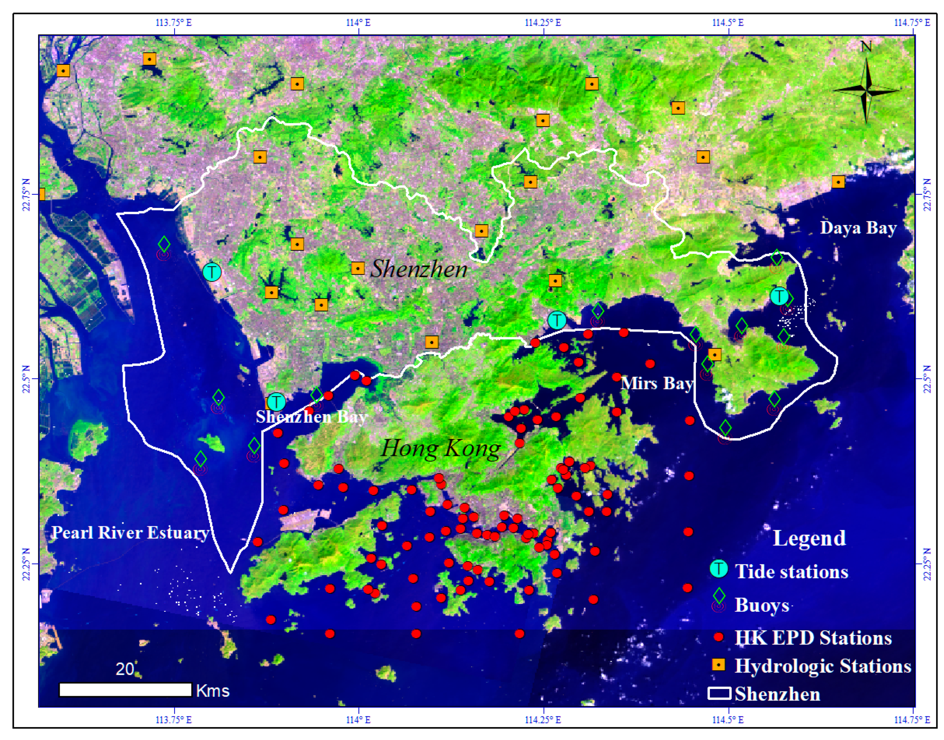
2. Shenzhen is located at the eastern shore of the Pearl River Estuary (PRE) and lies immediately North of Hong Kong. The coastal areas of Shenzhen consist of part of PRE and three major bays, i.e., Shenzhen Bay, Mirs Bay and Daya Bay. Figure 1 describes the coastal areas of Shenzhen. The coastal environment of Shenzhen is complicated by the huge amount of freshwater discharges from the PRE and polluted urban areas. The city has a subtropical marine climate. The annual average temperature is approximately 22 °C and the annual precipitation is 1933 mm.
Shenzhen was the first of China’s five Special Economic Zones in 1980. It then became the fastest growing city in China. Due to rapid population growth and economic development, loadings of pollutants into the costal water were greatly increased, and algal blooms occurred more frequently in the last three decades. A total of 162 HAB events were recorded in Shenzhen coastal areas from 1981 to 2014 [4]. The HABs events occurred most frequently from March to April. These algal blooms resulted in a large number of fish deaths and ecological damage. More than 40 algal species have been recorded to form red tides in Shenzhen, but most of them are harmless. The dominant algal species include skeletonema costatum, karenia mikimotoi, gyrodimium instriatum, and noctiluca scintillans. Algal species that cause harmful effects on fish include karenia digitate, chattonella marina and chattonella marina var. ovata.

3. Framework of the System

3.1. System Architecutre

HMFS was designed based on the concept of Service-Oriented Architecture (SOA). SOA is a conceptual architecture which includes collection of web services. These web services are loosely coupled and interoperable in a distributed computing environment. 
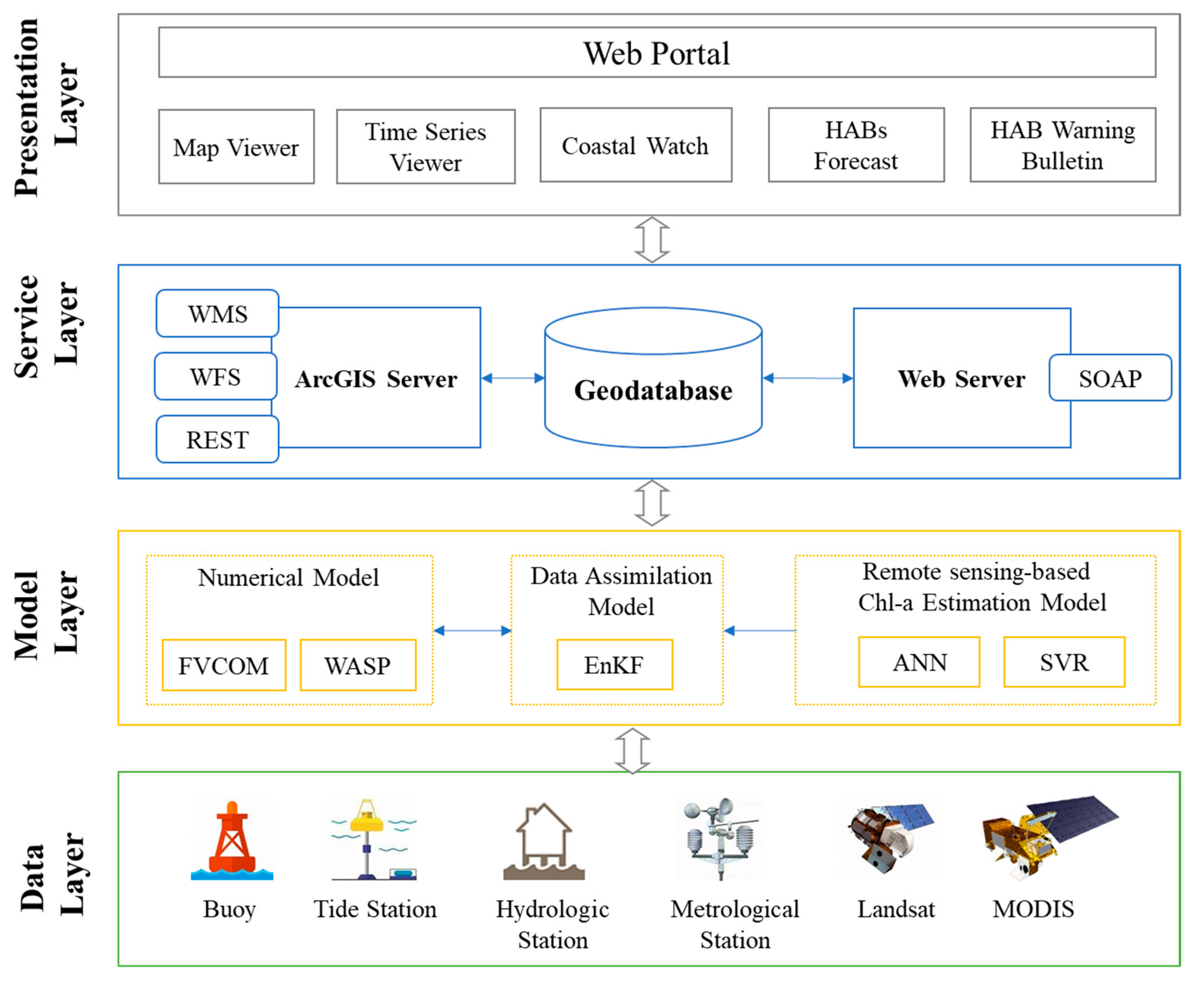
Figure 2 illustrates the service-oriented and multi-layer architecture of the system. The architecture is comprised of four layers: data layer, model layer, service layer, and presentation layer (or client layer).
The bottom layer contains a variety of data sources. The data sources could be grouped into two categories: satellite images and in situ observations. The satellite images (i.e., Landsat and MODIS) are regularly retrieved from online data repositories using Python script. The retrieved satellite images are processed and stored on the web server. The in situ observations measured at buoys, tide stations, hydrologic stations and metrological stations, are retrieved from the online system and stored in the geodatabase. In particular, real time data from in situ sensors are stored in the geodatabase following the Observations Data Model (ODM) specification [21]. ODM provides a standard to store and manipulate point observational data in a relational database.
The model layer forms the backbone of the system. It contains three types of models. The numerical hydrodynamic model coupled with a water quality model is driven by meteorological forecast data. The numerical model performs short-term prediction of hydrodynamic variables (e.g., water levels, currents, salinity, and water temperature) and water quality variables (e.g., Chl-a and dissolved oxygen). The remote-sensing-based Chl-a estimation models are used to estimate Chl-a spatial distribution by using machine learning algorithms. Currently, the available machine learning algorithms include Support Vector Regression (SVR) and Artificial Neuronal Network (ANN). Maps from remote sensing are directly saved in the geodatabase as raster. The data assimilation model is used to assimilate in situ and remote sensing observations into the numerical model by using the EnKF method, thereby reducing the mismatch between the model and observations.
The service layer provides web services through which the client can communicate with the server and retrieve data from the geodatabase. The geodatabase is a central data repository to store and manage all kinds of data, including time series at in situ stations, remote sensing maps and numerical model outputs. Geospatial data in the geodatabase is shared through ArcGIS Server web services. ArcGIS Server is a map server developed by Environmental Systems Research Institute (ESRI), Inc. It provides high-performance functionalities for end-users and developers to create, analyze and manage massive geospatial data. The ArcGIS Server enables clients to access data over the Internet through standard Open Geospatial Consortium (OGC) web services, including Web Map Service (WMS) and Web Feature Service (WFS). HMFS provides a variety of functionalities to query and retrieve point observations in the geodatabase. These functionalities are exposed to clients through Simple Object Access Protocol (SOAP) web services. In HMFS, the Web Server was built on Microsoft Internet Information Services (IIS) 10.0. Microsoft SQL Server2016 and Arc Spatial Database Engine (ArcSDE) were utilized to store and manage geospatial and time series of observational data.
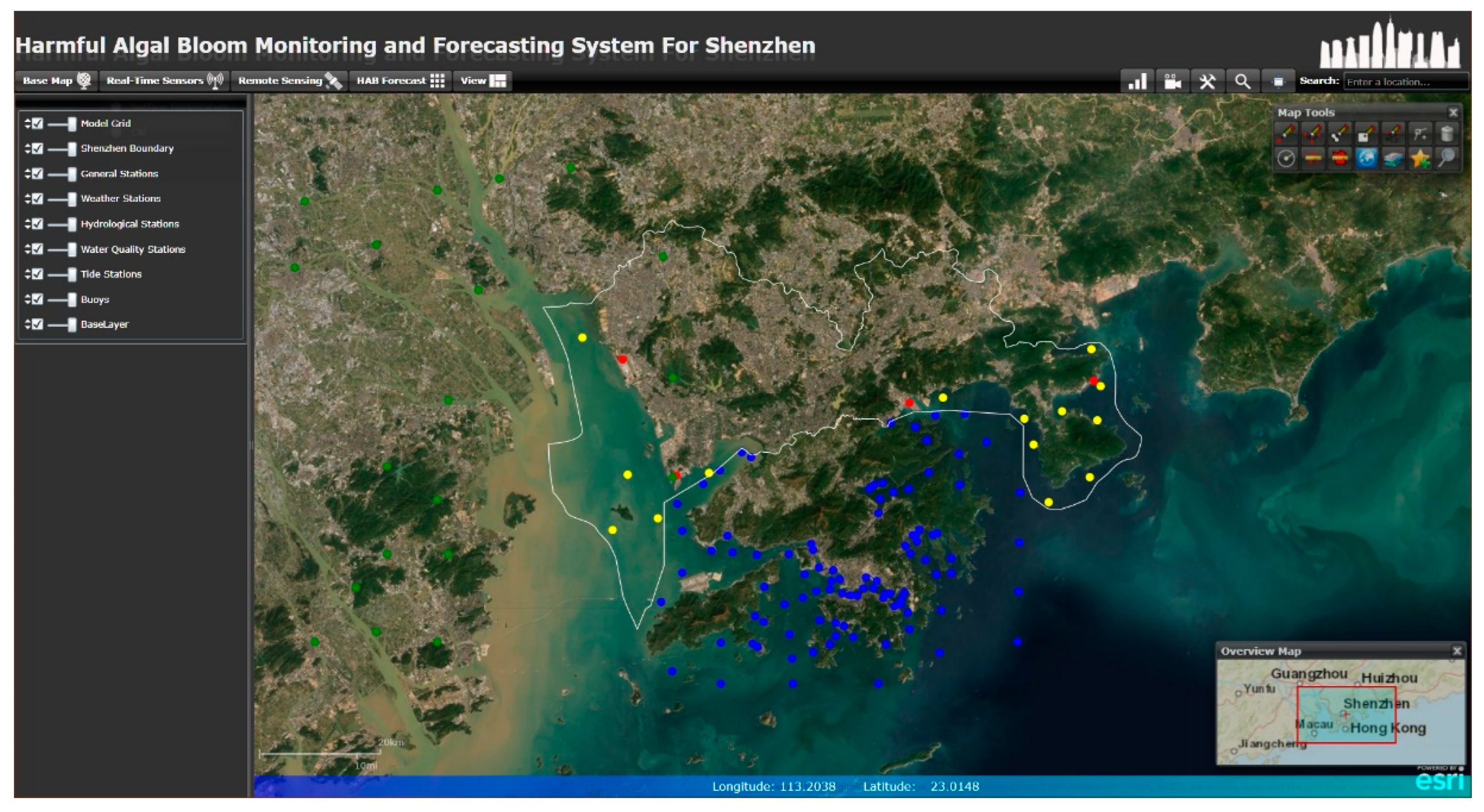
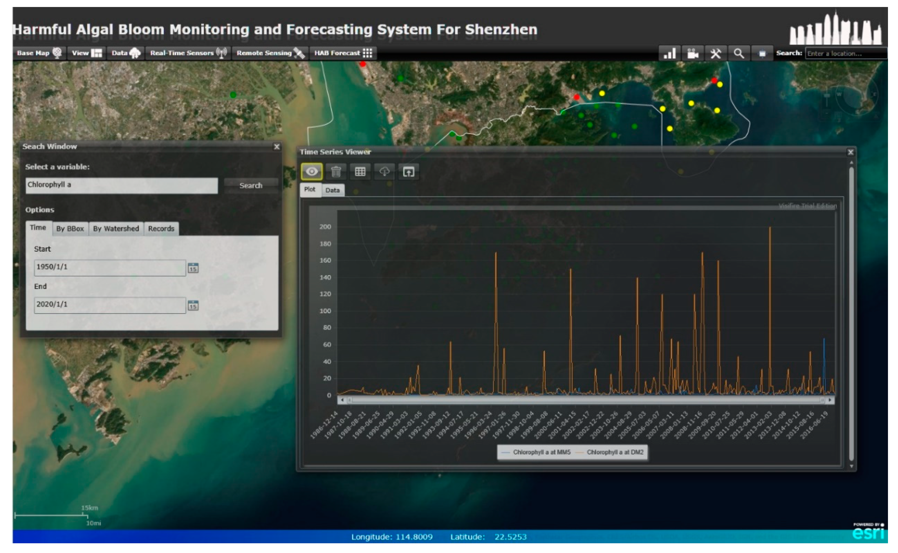
The presentation layer contains a web portal. The web portal was developed based on Microsoft ASP.NET. By making use of Rich Internet Applications (RIAs) technique, the web portal provides users with a highly interactive interface. The web portal contains a variety of tools, including map viewer, time series viewer, coastal watch, HABs forecast, and HAB warning bulletin. The web portal can be accessed through a common browser such as Internet Explorer.

3.2. In Situ Observation

The Shenzhen Planning and Natural Resources Bureau (SPNRB) has constructed a multi-sensor monitoring system to monitor coastal water conditions including tide and water qualities. Currently, the monitoring system consists of thirteen surface buoys and four tidal stations that are distributed along the coastline (see Figure 1). The real-time measurements from these in situ sensors are retrieved from the information system of SPNRB and stored in the geodatabase. In the study area, the Hong Kong Environmental Protection Department (EPD) has also implemented a water quality monitoring system which was initiated in 1986. The system consists of 94 routinely sampled stations for marine waters and 60 for bottom sediments, reporting marine water quality on a monthly basis. These monthly water quality measurements are very valuable for studying and understanding coastal and marine waters in Shenzhen and Hong Kong. Thus, these measurements are also routinely retrieved from the EPD website and archived in the geodatabase of the system.

3.3. Remote Sensing Based Estimation of Chlorophyll-a

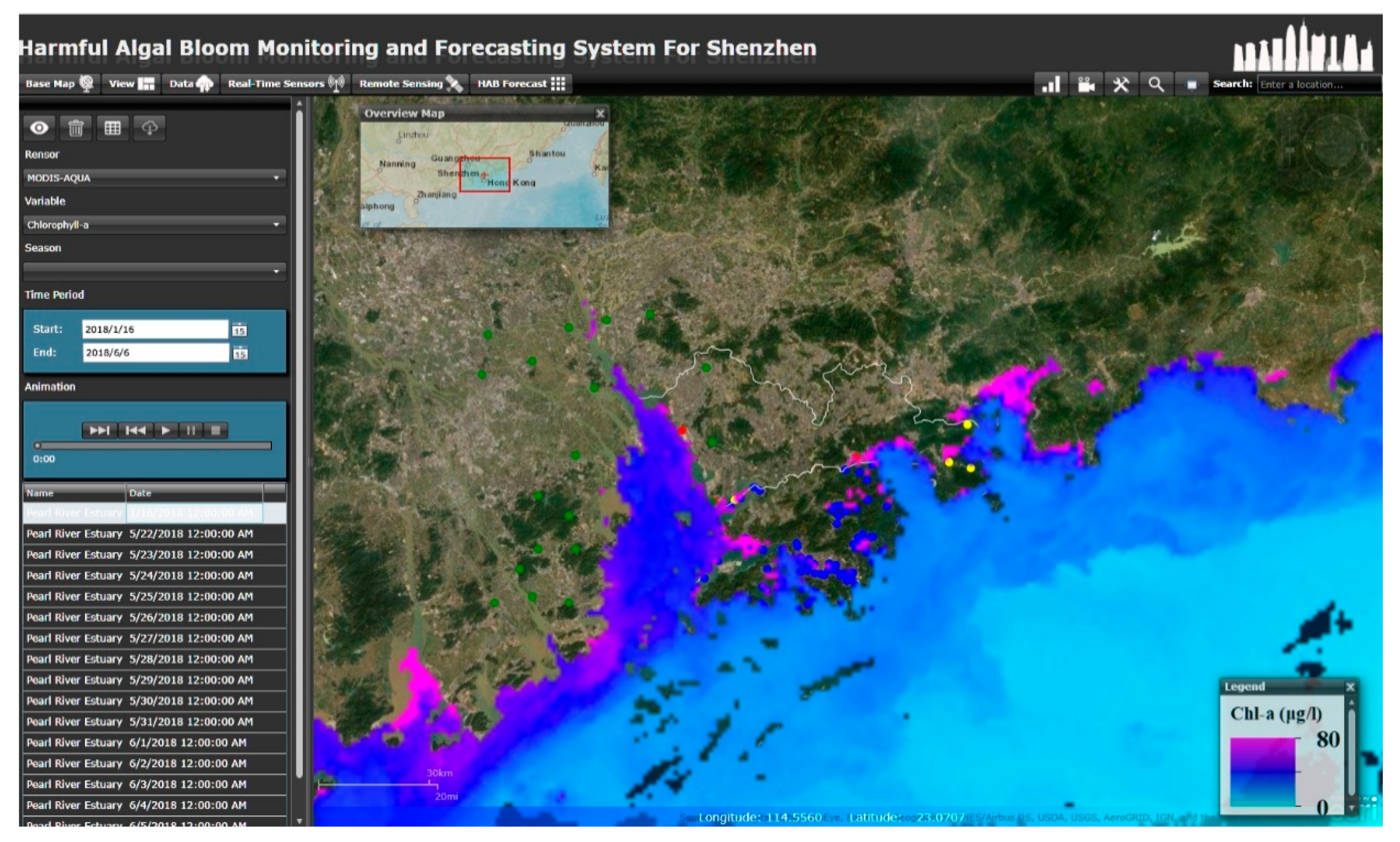
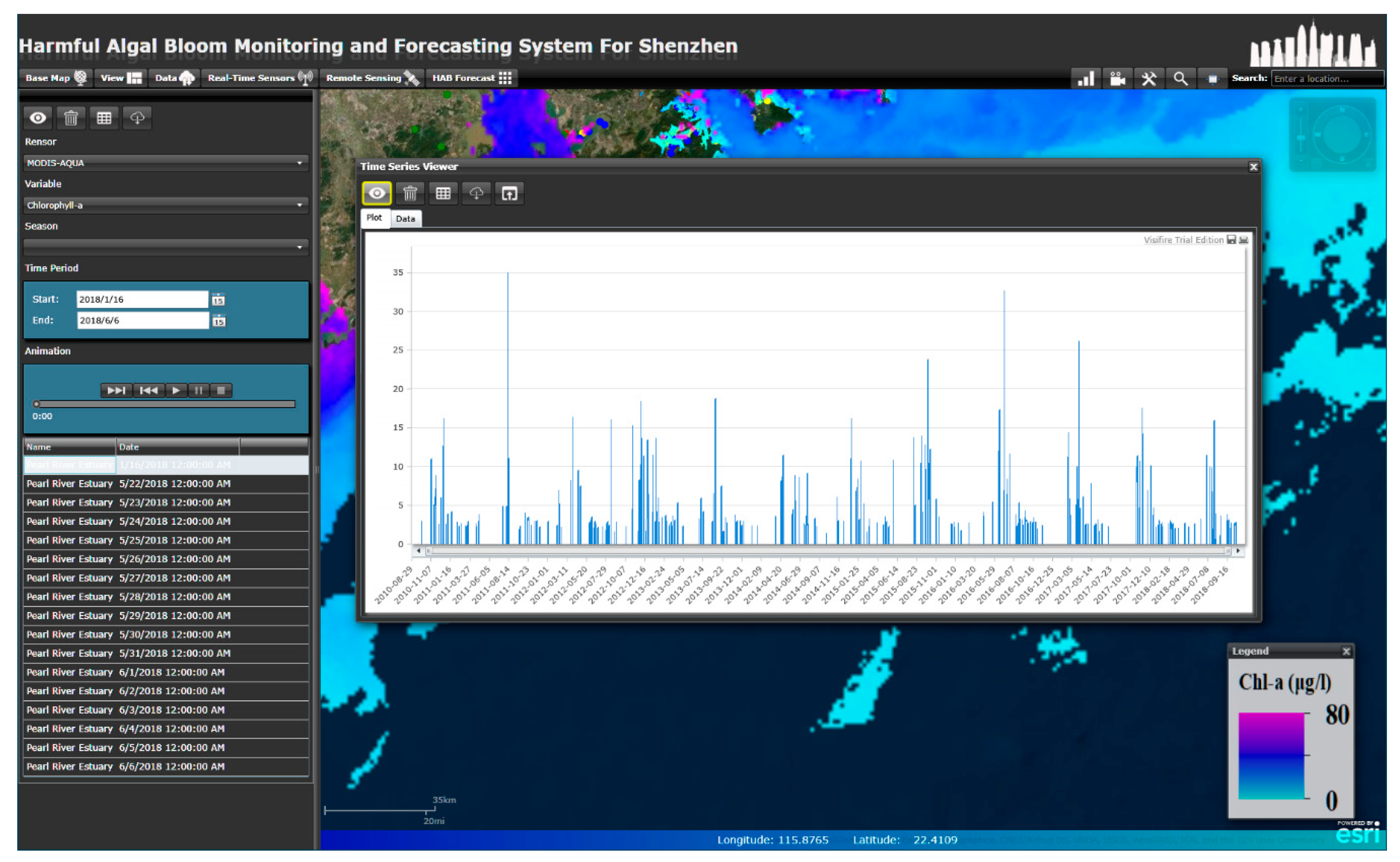
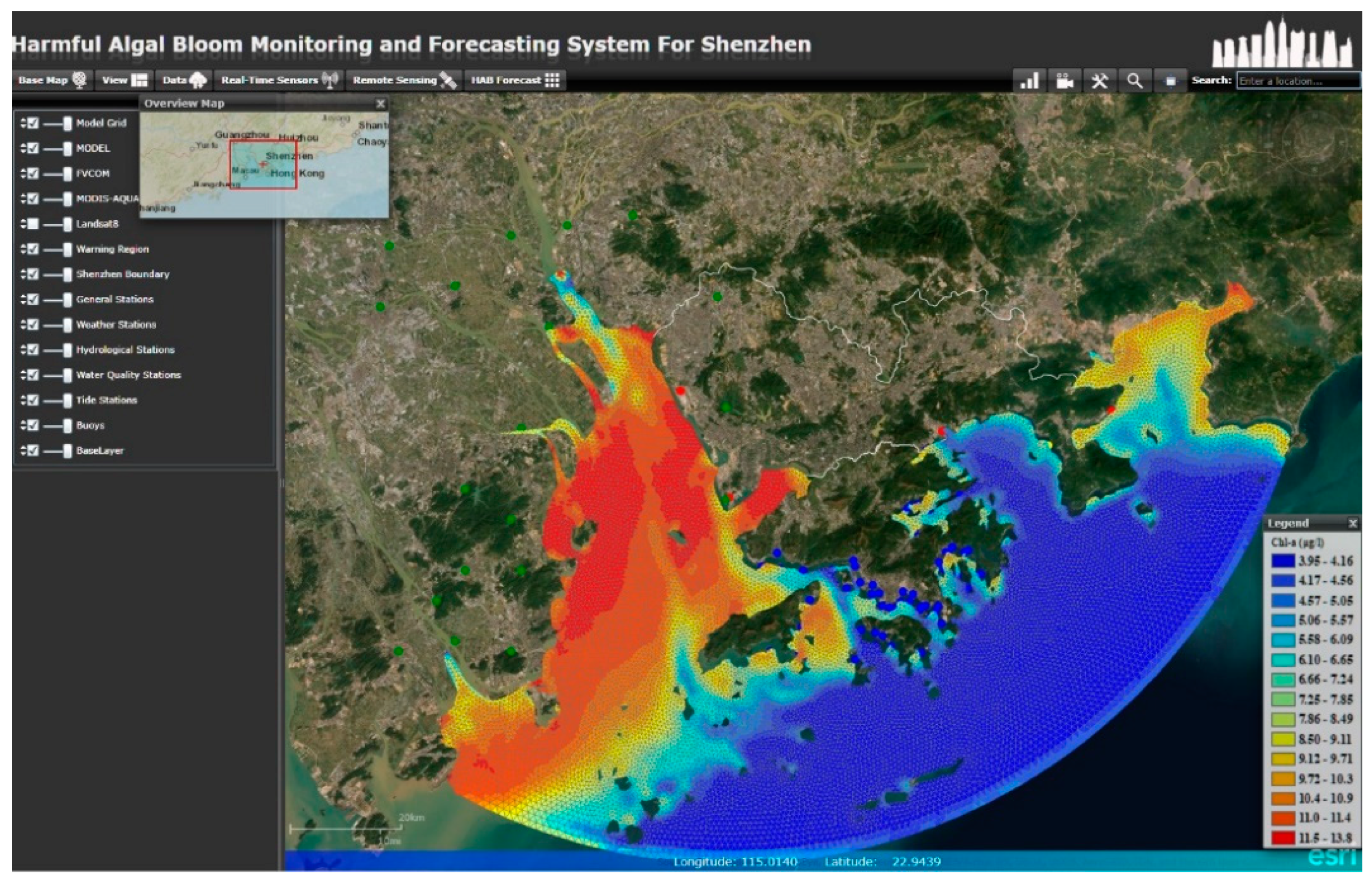
A potential algal bloom could be detected by anomalously high Chl-a concentrations in coastal waters [22]. Following this idea, Chl-a concentration was used as an indicator to detect and monitor HABs. Two types of remote sensing products are used to monitor HABs in HMFS. The first type adopts the standard MODIS Ch-l data products, which are generated and distributed by the Ocean Biology Processing Group (https://oceancolor.gsfc.nasa.gov) of National Aeronautics and Space Administration (NASA). The algorithm used to estimate surface water Chl-a in the NASA products combines a three-band difference algorithm for low Chl-a waters [23] with a band-ratio algorithm for high Chl-a waters [24]. The MODIS Chl-a data products have frequent revisit times (1–2 days) but have low spatial resolution (1 km).
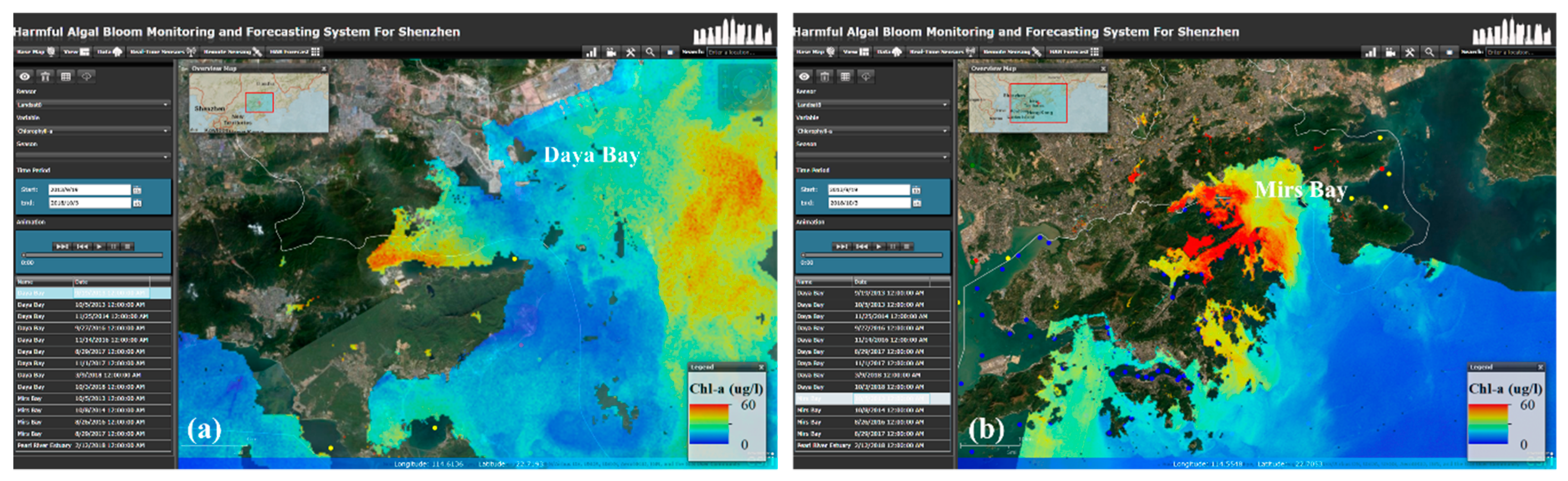
To provide a Chl-a distribution map with higher spatial resolution, Landsat images were also used in HMFS. Landsat sensors, including Thematic Mapper (TM) of Landsat-5 (L5), Enhanced Thematic Mapper Plus (ETM+) of Landsat-7 (L7) and Operational Land Imager (OLI) of Landsat-8 (L8), were used to estimate Chl-a in coastal waters. All the sensors have a spatial resolution of 30 m. Top of the Atmosphere (TOA) data L8, L7, and L5 were automatically downloaded from the Earth Explorer website (http://earthexplorer.usgs.gov/) through a Python routine, which is available at the website https://github.com/olivierhagolle/LANDSAT-Download. To remove atmospheric disturbances, atmospheric correction must be performed on the TOA data. Currently, a number of atmospheric correction methods are available. In HMFS, FLAASH (Fast Line-of-sight Atmospheric Analysis of Spectral Hypercubes) [25,26], an atmospheric correction modeling tool contained in ENVI (The ENvironment for Visualizing Images) software, was utilized to retrieve spectral reflectance (SR) from TOA images. FLAASH is one of the most popular atmospheric correction programs. It is developed based on the radiative transfer code, MODTRAN 4 (MODerate spectral resolution atmospheric TRANsmittance).
After performing the atmospheric correction, the spectral reflectance images were used to estimate chlorophyll-a concentration by using machine learning algorithms. The machine learning algorithms establish a relationship between in situ Chl-a concentrations and surface reflectance through training sets and then predict spatial distribution of Chl-a concentrations via the established relationship. In HMFS, two machine learning models were specially developed for Shenzhen coastal water, including Support Vector Regression (SVR) [27] and Artificial Neural Network (ANN). SVR is a popular machine learning algorithm for regression. SVR is able to deal with small sample size, non-linear and high-dimensional problems. It uses the same principle as the well-known Support Vector Machine (SVM), with minor differences. SVR develops a linear dependency between n input variables and one target variable by fitting an optimized hyper-plane. The remote sensing scenes over the Shenzhen coastal areas are often contaminated by cloud. Thus, the number of training samples is limited. Nevertheless, SVR has good generalization ability, even the number of training samples is small. In this study, Gaussian kernel was used in the SVR model. Several key parameters of SVR, including regularization parameter (C) and the loss function parameter (ε), were tuned through training processes until achieving the best prediction capabilities. ANN is another popular machine learning approach. It has been increasingly used to forecast algal blooms because of its capabilities in forecasting complex relationships [28,29]. ANN applied in this study consists of an input layer with Np nodes, a hidden layer with Nh nodes, and an output layer with one node. Np is the number of input variables which depend on the selected surface reflectance bands. Nh is the number of neuron nodes in the hidden layer. The tangent sigmoid function was chosen as the transfer function between the hidden and output layers.

3.4. Numerical Models for HAB Forecasting

The numerical models for HAB forecasting consist of a hydrodynamic model, a water quality model and a data assimilation model. FVCOM (version 3.1.6) was used to establish the hydrodynamic model. FVCOM is an unstructured-grid and finite-volume ocean model with a terrain-following coordinate system in the vertical and a triangular grid in the horizontal. It can be easily customized due to its open source policy. FVCOM enables modelling of hydrodynamics variables including water level, current, water temperature, and salinity. A great advantage of FVCOM is that it enables the use of unstructured triangular grids to accurately fit the complex coastlines, such as the Peral River Estuary and the Shenzhen coastal areas. FVCOM is numerically solved using a split-mode method. The source code of FVCOM is parallel, and a Message Passing Interface (MPI) is used as the message passing system. FVCOM has been successfully applied to coastal areas [30,31], estuaries [32], and data assimilation studies [14,33].
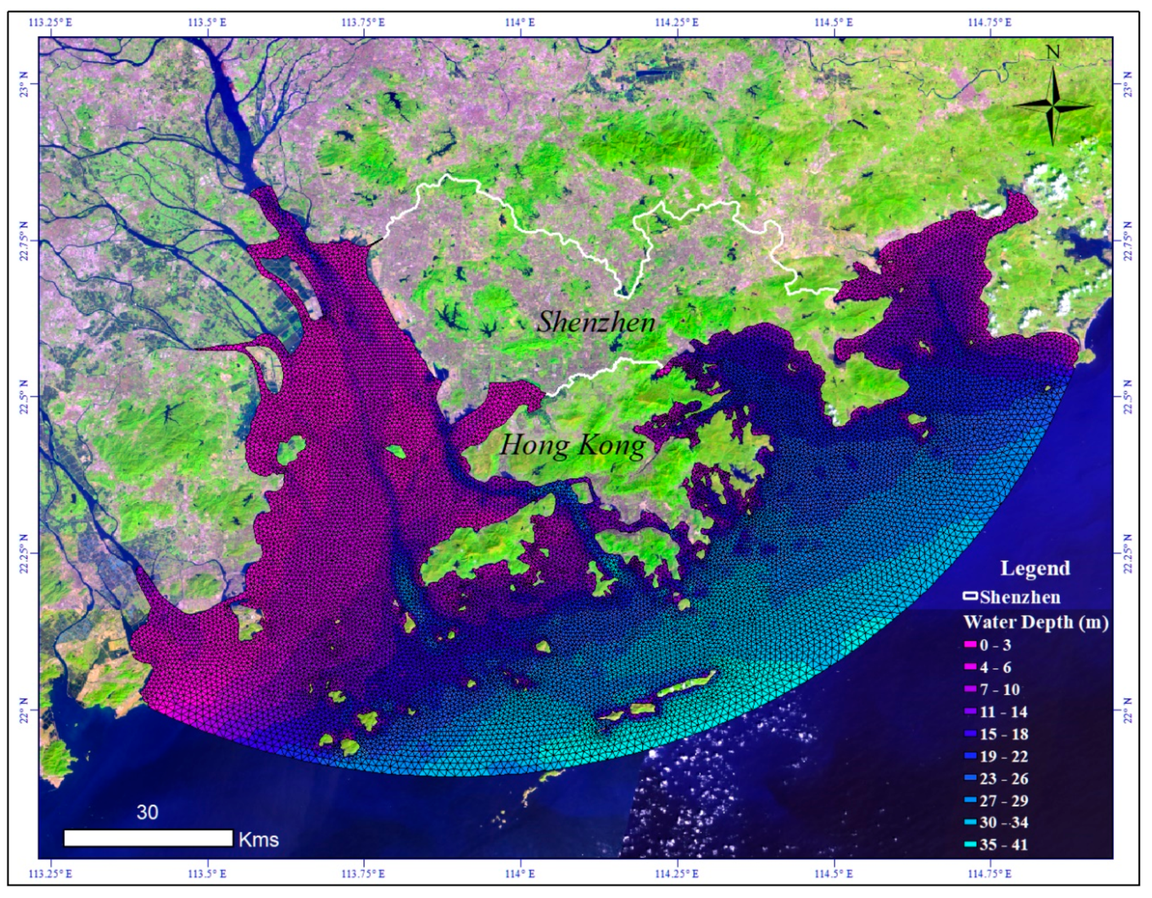
The modeling domain and discretized grid in this study are presented in Figure 3. The domain includes the Pearl River Estuary and the coastal areas around Shenzhen and Hong Kong. Horizontally, the grid consists of 15,351 nodes and 28,880 triangular cells. The spatial resolution of the horizontal cells ranges from 400 m to 1500 m. The triangular cells along the coast have finer resolution, while the cells at the offshore open boundary have a coarser resolution. Vertically, the model has nine terrain-following layers. The model bathymetry is derived from the General Bathymetric Chart of the Oceans. Triangular cells with a depth of less than 1 m occupy less than 1%; therefore, the minimum depth was set to 1 m. The modified Mellor and Yamada level-2.5 (MY-2.5) was chosen as the turbulent closure scheme. Parameters of the MY-2.5 scheme and the non-dimensionless viscosity parameter in the Smagorinsky formula were set according to the ones used in other similar FVCOM models. On the basis of the Courant–Friedrichs–Lewy (CFL) criterion, an integration time step of 5 s was set for the external mode and the time step of the internal mode was set to 50 s [34,35].
The water quality model used in this study is the Water Analysis Simulation Program (WASP). WASP simulates eight water column state variables, including dissolved oxygen (DO), nitrate and nitrite (NO2 and NO3), ammonia (NH3), organic nitrogen (ON), organic phosphorus (OP), inorganic phosphorus (OPO4), carbonaceous biochemical oxygen demand (CBOD), and chlorophyll-a (Chl-a). The governing equations of the WASP are described in detail in [22]. The WASP was coupled with FVCOM and can be run in an online mode. The parameter values of the WASP model were specified based on literature reviews [4,36,37] and previous WASP applications [38].
The coupled model was driven by meteorological data, including precipitation, air pressure, temperature, relative humidity, and evaporation. The meteorological data was derived from the European Center for Medium-Range Weather Forecast (ECMWF) datasets (available at http://www.ecmwf.int). ECMWF produces global numerical weather predictions four times per day. Tidal forcing was considered by specifying eight major tidal constituents at the offshore open boundary. The tidal constituents include M2, N2, S2, K2, K1, O1, P1, and Q1. These tidal constituents were determined by interpolating the 1/6° inverse tidal model results generated by Tidal Inversion Software (OTIS) [39]. Freshwater and nutrient fluxes from the major river inlets were used as boundary conditions. River flow rate forecasts were generated using machine learning algorithms based on daily discharges observations obtained from Pearl River Water Resources Commission. Water quality constituent fluxes were derived based on weekly measurements at the river inlets, obtained from the Department of Ecology and Environment of Guangdong Province.
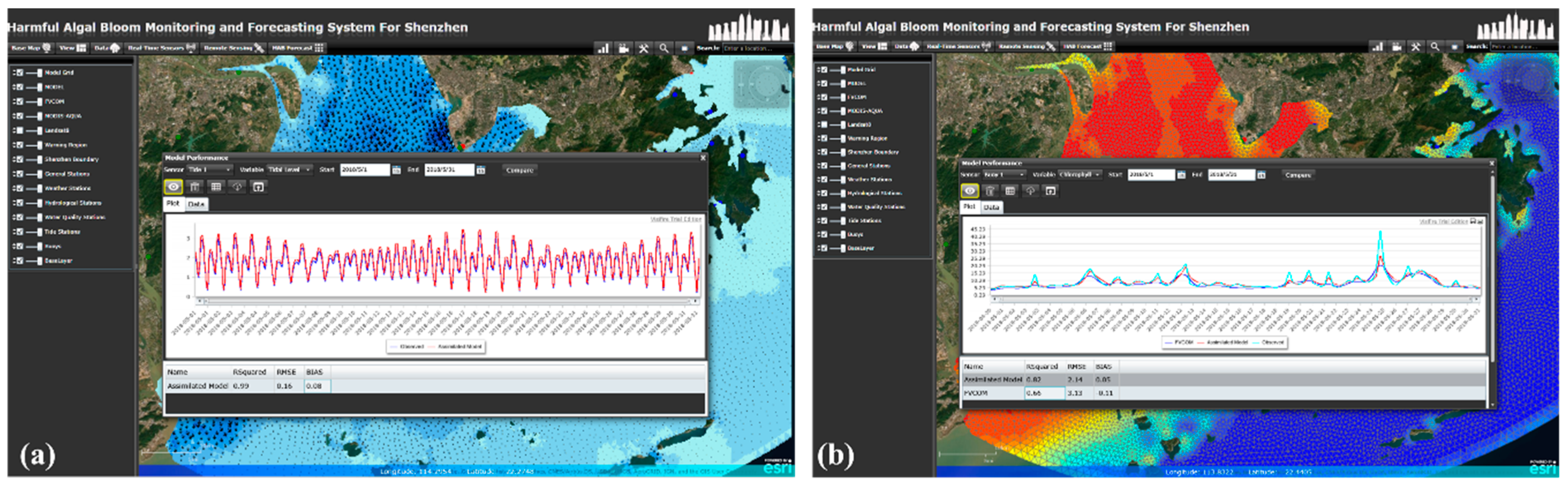
The coupled model was calibrated by comparing simulated hydrodynamic variables (i.e., tidal level and water temperature) and water quality variables (i.e., Chl-a and DO) against observation values. The observational data sets in 2017 were used to perform the calibration. The hydrodynamic model parameters (e.g., roughness coefficients) and the WASP model parameters were adjusted during the calibration until good agreement between the simulation results and the observations was achieved.
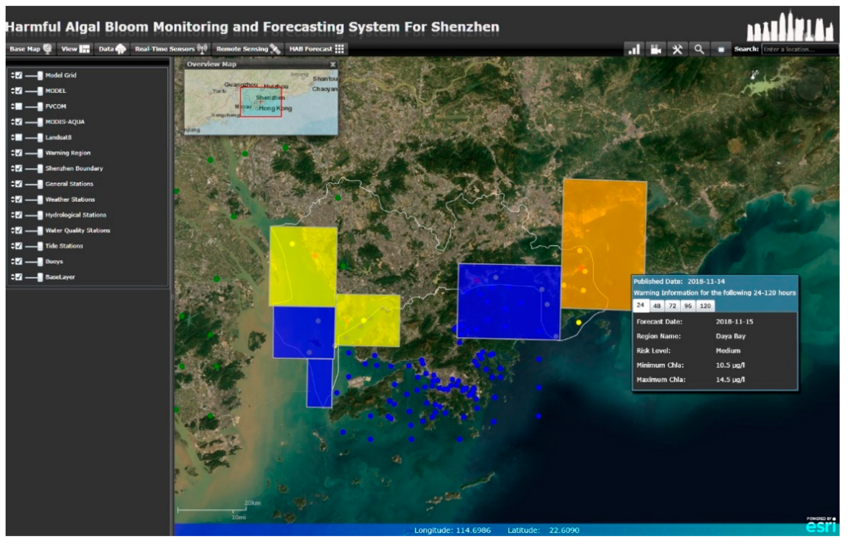
For an operational system, it is useful to implement a sequential data assimilation algorithm, through which the observations can be assimilated as they become available. To this end, a popular data assimilation scheme, EnKF, was employed to assimilate the Chl-a concentration observed at in situ stations and derived from remote sensing observations into the numerical model. In HMFS, the EnKF ensemble was generated by perturbing meteorological driving force fields. High-Performance Computing (HPC) environments were employed to run the model since the numerical models are computationally and data-intensive. Outputs from both the free model run (without assimilation) and assimilated model run were achieved on the HPC cluster using netCDF (network Common Data Form) file format, which is a widely used format for storing scientific data. The numerical models produce a 3–5 days forecast of hydrodynamics and Chl-a distribution, and the possible HAB event occurrence was determined by comparing the forecasted Chl-a concentration with a predefined threshold. The threshold could be defined by decision-makers. Currently, a potential HAB event triggering for the Shenzhen coastal region was set with current Chl-a concentration greater than 15 μg/L.

3.5. Data Post-Processing and Publication

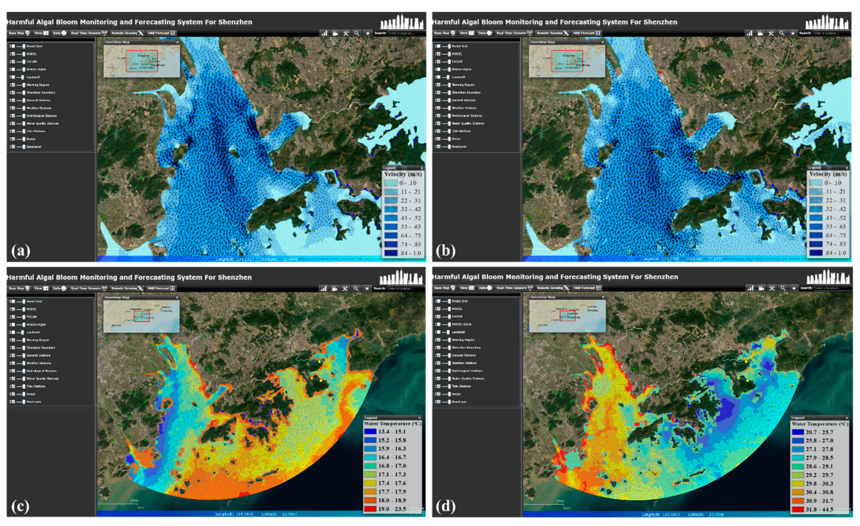
In HMFS, the raw modeling outputs achieved on the cluster are pushed to the web server via FTP (File Transfer Protocol) and are automatically processed by a post-processing tool. The tool was developed using C# and deployed on the server-side. It was used to convert model outputs in the netCDF format to GIS raster/feature layers and store the converted data sets in the geodatabase. Table 1 lists GIS layers automatically generated by the post-processing tool. To provide better visualization effects, rendering style is pre-designed for each kind of variable. The raster layers are symbolized by classification/stretch rendering with color ramps. Current filed (velocity and direction) is symbolized with arrows. The generated GIS layers are then published via ArcGIS Server.

4. Web Portal

4.1. Overview of the Web Portal

Figure 4 depicts the graphic user interface (GUI) of the web portal. The web portal has a layout and GUI elements that are similar to desktop applications. It allows users to perform various operations in a single web page. The GUI was developed using the ArcGIS API (Application Program Interface) for Silverlight, which provides advanced functionalities for creating a rich interactive user interface and contains comprehensive libraries for charting, mapping and geospatial analyzing. As shown in Figure 4, the map viewer occupies the main frame of the GUI. Other interactive interface components include menus, toolbox, floating windows, tables and so on. Many of the components are floated on the map viewer and can be turned on or turned off as required.
The map viewer plays a central role in integrating and visualizing all kinds of geospatial data. The map viewer supports fluent common map operations such as pan, zoom in/out, bookmarks, measure, and overview. Geospatial data displayed in the map viewer are organized as layers. The layers are displayed and managed by the layer manger, which is located on the left side of the GUI in Figure 4. The layer manager allows users to adjust layer display orders, toggle layer visibility and set layer opacity. The web portal provides a set of base map layers, including world imagery, roads, terrain and others. These base map layers are retrieved from ArcGIS Online. After launching the web portal, a default base map will be displayed.
Besides the map viewer, other important tools provided in the web portal include time series viewer, Coastal Watch, and HAB forecast and warning tools, which are described in the following sections.

4.2. Explorering Observational Time Series

The web portal provides several functionalities to display monitored information. For real-time sensor data, sensors’ location and descriptions are displayed on the map viewer (see Figure 5). The latest measurements at each sensor are updated at a given time interval. By clicking on a sensor, details about the sensor will be displayed in a popup window.
The web portal provides a tool to help users search, explore and analyze historical observational time series. Users can use the search box to query time series of a concern variable within an area of interest (AOI). After specifying a variable in the keyword box and selecting an AOI, stations measuring the variable will be displayed in the map viewer through point symbols. When clicking on the station, a pop-up window will be displayed to show detailed information about the station. Time series of the specified variable at the select station will also be retrieved from the remote geodatabase and be plotted in the time series viewer. The time series can also be viewed in a data table and can be downloaded to a local computer with the format of Comma Separated Value (CSV). The time series viewer allows multiple time series to be plotted in a single chart. Figure 5 presents the plot of time series of Chl-a measured at two stations named MM5 and DM2. The DM2 station is located in the Shenzhen Bay and the MM5 station is located in the Daya Bay. It can be found that the Chl-a concentration in the Shenzhen Bay is significantly higher than that in the Daya Bay.

4.3. Visualization of Remote-Sensing Estimated Chlorophyll-a

The Costal Watch tool in the web portal enables the user to view and explore images of Chl-a concentration that are estimated based on remote sensing. By selecting a sensor and a variable, the available images labeled with dates will be listed in a table. Clicking on a date in the table, the corresponding image will be displayed in the map viewer. Figure 6 depicts Chl-a distribution from MODIS-Aqua products over Shenzhen coastal areas on 16 January 2018. The web portal provides a probe tool to extract time series at a user-specified location from a certain image product. Figure 7 shows a time series of Chl-a from the MODIS-Aqua products at a location in the Shenzhen Bay during the period from 2010 to 2018.
The spatial resolution of MODIS-Aqua products is relatively coarse (1000 m). The Landsat images are able to provide more detailed spatial distribution of Chl-a. Several extensive HABs occurred around Shenzhen coastal areas in last ten years. Figure 8 presents maps of Chl-a concentration estimated by the SVR approach under two typical HAB events. A massive HAB occurred during November 2014 in the Daya Bay. Figure 8a presents mapping of Chl-a concentration on 25 November 2014 in the Daya Bay. It can be seen that the water areas affected by the HAB had an anomalously high Chl-a concentration ranging from 20 to 60 μg/L. Figure 8b displays a HAB which occurred on 29 August 2017 in the Mirs Bay.

4.4. Visualization of Forecasting Data

The numerical forecasting results can be viewed and explored in the web portal through the forecast data manger. By selecting a variable and a date in the manger, the spatial distribution of the variable will be visualized in the map viewer. Figure 9a,b present simulated sea surface currents during flood and ebb tides by the assimilated model run. It can be seen that the velocity of the flood tide was less than the ebb tide and the directions of flood and ebb tides were opposing. Figure 9c,d present a simulated sea surface temperature (SST) in the modeling domain on 10 January 2018 (dry season) and on 10 July 2018 (wet season), respectively. By comparing the modeling results with previous studies [40,41], it was found that the hydrodynamic model of HMFS has reasonable skill in simulating sea current and temperature. Figure 10 presents spatial distribution of assimilated Chl-a on 10 July 2018. As the hydrodynamics and water quality of coastal water is continuously changing, animation of the modeling outputs is helpful for the user to view and understand the complex ocean processes. The forecast data manger enables the animation of forecast data over a selected time span.
The web portal provides a tool that enables the user to investigate model performance by comparing simulated and observed hydrodynamic and water quality variables at a selected location for a time span. Figure 11a presents comparison between observed tidal level and simulated tidal level by the assimilated model run at the T1 tide station from 1 May to 31 May, 2018. The goodness-of-fit is indicated by several statistical measures, including the coefficient of determination (R2), percentage bias (BIAS) and Root Mean Square Error (RMSE). These statistical measures are automatically calculated by the tool when performing the compassion. For the compassion shown in Figure 11a, the R2, BIAS, and RMSE are equal to 0.99, 0.08, and 0.16 m, respectively, indicating that the hydrodynamic model can reproduce tidal variation very well. A Chl-a comparison among free model run, assimilated model run and in situ observation from 1 May to 31 May 2018 is given in the tool (Figure 11b). The R2, BIAS and RMSE between free model run (i.e., FVCOM) and observation are equal to 0.66, −0.11, and 3.11 μg/L, respectively. The R2, BIAS and RMSE between assimilated model run and observation are equal to 0.82, 0.05, and 2.14 μg/L, respectively. It can be seen that the assimilated model simulates the Chl-a concentration with greater accuracy.
The HAB warning bulletin tool generates warning information based on a 5-days forecast of Chl-a produced by the operational numerical model. The HAB warning information is displayed in the map viewer, as shown in Figure 12. The risk level of a possible HAB event is represented with different colors. In HMFS, the risk of a HAB event is classified into four levels according to the value of Chl-a concentration: (1) Very low risk, indicated by blue color and Chl-a concentration ranging from 0 to 5 μg/L; (2) low risk, indicated by yellow color and Chl-a concentration ranging from 5 to 10 μg/L; (3) medium risk, indicated by orange color and Chl-a concentration ranging from 10 to 15 μg/L; and (4) high risk, indicated by red color and Chl-a concentration greater than 15 μg/L.
The HMFS began a trial operation in 2018. A simple score introduced by Silva et al. [42] was used to evaluate the forecast accuracy of the system. The score is calculated as follows:
ε = i = 1 n f i n 100 % ,   where { f = 1 ,   if   True f = 0 ,   if   False
where n is the total number of forecasts; True means that a predicted HAB event matches the observation and False means the opposite situation. The False is further classified into two categories: False positive indicates that a predicted HAB event does not occur; and False negative indicates that a HAB event is observed but is not correctly predicted.
Figure 13 shows the forecast accuracies in the four coastal areas of Shenzhen during 2018. The total number of forecast attempts in the Shenzhen Bay, Mirs Bay, Daya Bay, and Pearl River Estuary (PRE) are 3, 2, 4, and 4. It can be seen that Shenzhen Bay and PRE had higher accuracy scores, while Mirs Bay and Daya Bay had lower accuracy scores. Overall, the forecast accuracy scores were more than or equal to 50%. The False positives and negatives forecasts were obtained in all of the four areas. However, relying solely on Chl-a concentration for HAB warning may cause incorrect forecast. According to observations, HAB events that occurred in the Shenzhen Bay and PRE had larger extents but had lower frequency. By comparison, HAB events that occurred in the Mirs Bay and Daya Bay had smaller extents but had higher frequency. The system had better forecast performance in the Shenzhen Bay and PRE because Chl-a concentration tended to be a good indicator in these two areas. However, in addition to Chl-a concentration the occurrence of HAB in the Mirs Bay and Daya Bay was also affected by other environmental factors including wind, water temperature and nutrients. It was more difficult for the system to predict HABs in these two areas.
Figure 14 presents forecast results of two actual HAB events in the Shenzhen coastal areas. Figure 14a presents a successful forecast of HAB that occurred in the Pearl River Estuary during 1–10 November, 2018. It can be seen that the simulated Chl-a concentration in the area affected by the HAB event (indicated by a red rectangle) is higher than 40 μg/L. According to the HAB report provided by SPNRB, this HAB event lasted over 10 days and the area affected by the HAB event was approximately 20 km2. Both of the extent and intensity of the HAB event were successfully simulated by the system. However, the system may not provide effective early warning if the scale of HAB is very small. An example of failure warning is given in Figure 14b. According to the report provided by SPNRB, a HAB event occurred in the Mirs Bay during 5–8 March, 2018, and the area affected by the event was no more than 0.1 km2. The system did not capture this event. More environmental factors (e.g., water temperature and nutrients) need to be considered when performing the forecast.

5. Conclusions

In this study, we introduced an integrated web-based system for the monitoring and forecasting of coastal HABs. The system provides a web-based environment to monitor and forecast HABs by leveraging remote sensing, numerical modeling, and Web-GIS technologies. The system allows end-users to view the in situ observations, remote sensing maps and numerical model forecasts in a geospatial context. The application of the system can improve the understanding of the hydrodynamic and water quality processes in the Shenzhen coastal areas and may reduce potential economic and health losses arising from the occurrence of HABs events.
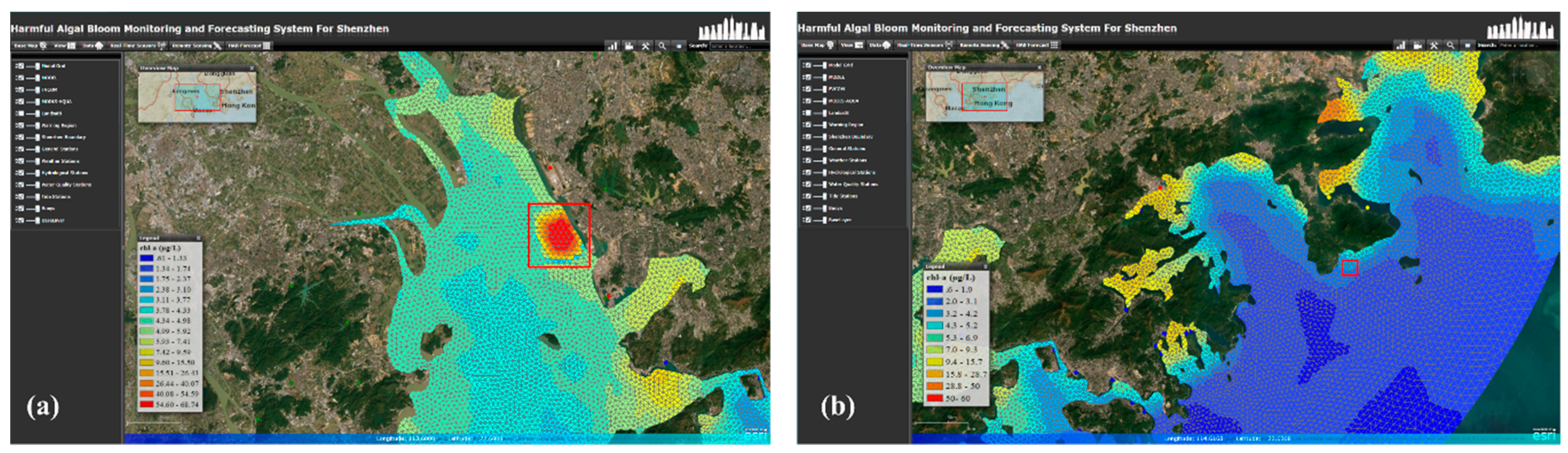
The system was successfully applied to detect coastal HABs events using the remote sensing models. The remote sensing models were proven to be effective by identification of anomalously higher Chl-a concentrations. They can be used to perform routine monitoring of HAB events in the complex coastal areas of Shenzhen. The forecast results illustrate that the numerical model, in combination with the EnKF assimilation algorithm, is successful in predicting hydrodynamics and water quality processes up to 5 days. By leveraging Web-GIS, RIAs, and SOA technologies, the web portal of the system provides a single map-based interface, in which data of different types (point time series, vector, and raster) can be visualized and analyzed through interactive tools. The source code of the web portal could be found at the link https://github.com/DeepHydro.
Although the system was specially developed for Shenzhen coastal areas, it can be adapted to other coastal regions where monitoring and forecasting of HABs are required. However, the numerical models have to be established and calibrated for the region of interest, and the software environments (i.e., GIS server and geodatabase) have to be deployed and configured by developers. In future work, routine monitoring of Chl-a based on remote sensing will be improved by employing more sensors, such as Japanese Himawari-8, European Space Agency (ESA) sentinel 2/3 and Chinese HJ-1 A/B. The numerical models also need to be improved, for example, the hydrodynamic model should better simulate typhoon or tropical storms and the water quality model should better simulate the ecosystem in the sea water. We noticed that ArcGIS API for Silverlight may not be the best option for the system. ArcGIS API for JavaScript, the new generation of ESRI’s technology for web GIS development is a better choice since it provides better performance and supports the HTML5 (Hypertext Markup Language5). To meet the needs of mobile Internet applications, we plan to develop a new version of the web portal via ArcGIS API for JavaScript and HTML5 platform.

Author Contributions

Conceptualization, M.H.; Methodology, Y.T.; Software, Y.T.; Writing—original draft, Y.T.; Writing—review and editing, M.H.

Funding

This research was funded by the National Natural Science Foundation of China (No. 41890852 and No. 51579108), the Shenzhen Science and Technology Innovation Commission (No. JCYJ20160530190547253) and the National Key Research and Development Program of China (No. 2017YFC0405900). Additional support was provided by the Fundamental Research Funds for the Central Universities (No. 2017KFYXJJ203).

Conflicts of Interest

The authors declare no conflict of interest.

References

  1. Anderson, D.M. Approaches to monitoring, control and management of harmful algal blooms (HABs). Ocean Coast. Manag. 2009, 52, 342–347. [Google Scholar] [CrossRef] [PubMed] [Green Version]
  2. Wang, J.H.; Wu, J.Y. Occurrence and potential risks of harmful algal blooms in the East China Sea. Sci. Total Environ. 2009, 407, 4012–4021. [Google Scholar] [CrossRef] [PubMed]
  3. Huang, J.; Liu, H.; Yin, K. Effects of meteorological factors on the temporal distribution of red tides in Tolo Harbour, Hong Kong. Mar. Pollut. Bull. 2018, 126, 419–427. [Google Scholar] [CrossRef] [PubMed] [Green Version]
  4. Song, X.Y.; Huang, L.M.; Zhang, J.L.; Huang, H.H.; Li, T.; Su, Q. Harmful algal blooms (HABs) in Daya Bay, China: An in situ study of primary production and environmental impacts. Mar. Pollut. Bull. 2009, 58, 1310–1318. [Google Scholar] [CrossRef] [PubMed]
  5. Gregg, W.W.; Casey, N.W. Global and regional evaluation of the SeaWiFS chlorophyll data set. Remote Sens Environ 2004, 93, 463–479. [Google Scholar] [CrossRef]
  6. Vilas, L.G.; Spyrakos, E.; Palenzuela, J.M.T. Neural network estimation of chlorophyll a from MERIS full resolution data for the coastal waters of Galician rias (NW Spain). Remote Sens. Environ. 2011, 115, 524–535. [Google Scholar] [CrossRef]
  7. Gitelson, A.A.; Dall’Olmo, G.; Moses, W.; Rundquist, D.C.; Barrow, T.; Fisher, T.R.; Gurlin, D.; Holz, J. A simple semi-analytical model for remote estimation of chlorophyll-a in turbid waters: Validation. Remote Sens. Environ. 2008, 112, 3582–3593. [Google Scholar] [CrossRef]
  8. Song, C.; Woodcock, C.E.; Seto, K.C.; Lenney, M.P.; Macomber, S.A. Classification and change detection using Landsat TM data: When and how to correct atmospheric effects? Remote Sens. Environ. 2001, 75, 230–244. [Google Scholar] [CrossRef]
  9. Sriwongsitanon, N.; Surakit, K.; Thianpopirug, S. Influence of atmospheric correction and number of sampling points on the accuracy of water clarity assessment using remote sensing application. J. Hydrol. 2011, 401, 203–220. [Google Scholar] [CrossRef]
  10. Nazeer, M.; Nichol, J.E. Development and application of a remote sensing-based Chlorophyll-a concentration prediction model for complex coastal waters of Hong Kong. J. Hydrol. 2016, 532, 80–89. [Google Scholar] [CrossRef]
  11. Davidson, K.; Anderson, D.M.; Mateus, M.; Reguera, B.; Silke, J.; Sourisseau, M.; Maguire, J. Forecasting the risk of harmful algal blooms Preface. Harmful Algae 2016, 53, 1–7. [Google Scholar] [CrossRef] [PubMed]
  12. Chen, C.S.; Gao, G.P.; Zhang, Y.; Beardsley, R.C.; Lai, Z.G.; Qi, J.H.; Lin, H.C. Circulation in the Arctic Ocean: Results from a high-resolution coupled ice-sea nested Global-FVCOM and Arctic-FVCOM system. Prog. Oceanogr. 2016, 141, 60–80. [Google Scholar] [CrossRef] [Green Version]
  13. Waldman, S.; Bastón, S.; Nemalidinne, R.; Chatzirodou, A.; Venugopal, V.; Side, J. Implementation of tidal turbines in MIKE 3 and Delft3D models of Pentland Firth & Orkney Waters. Ocean Coast. Manag. 2017, 147, 21–36. [Google Scholar] [CrossRef] [Green Version]
  14. Chen, C.S.; Malanotte-Rizzoli, P.; Wei, J.; Beardsley, R.C.; Lai, Z.G.; Xue, P.F.; Lyu, S.J.; Xu, Q.C.; Qi, J.H.; Cowles, G.W. Application and comparison of Kalman filters for coastal ocean problems: An experiment with FVCOM. J. Geophys. Res. Ocean. 2009, 114. [Google Scholar] [CrossRef] [Green Version]
  15. Xie, J.; Zhu, J. Ensemble optimal interpolation schemes for assimilating Argo profiles into a hybrid coordinate ocean model. Ocean Model. 2010, 33, 283–298. [Google Scholar] [CrossRef]
  16. Pan, C.D.; Zheng, L.Y.; Weisberg, R.H.; Liu, Y.G.; Lembke, C.E. Comparisons of different ensemble schemes for glider data assimilation on West Florida Shelf. Ocean Model. 2014, 81, 13–24. [Google Scholar] [CrossRef]
  17. Aunsri, N.; Chamnongthai, K. Particle filtering with adaptive resampling scheme for modal frequency identification and dispersion curves estimation in ocean acoustics. Appl. Acoust. 2019, 154, 90–98. [Google Scholar] [CrossRef]
  18. Kulawiak, M.; Prospathopoulos, A.; Perivoliotis, L.; Luba, M.; Kioroglou, S.; Stepnowski, A. Interactive visualization of marine pollution monitoring and forecasting data via a Web-based GIS. Comput. Geosci. 2010, 36, 1069–1080. [Google Scholar] [CrossRef]
  19. Qin, R.F.; Lin, L.Z. Development of a GIS-based integrated framework for coastal seiches monitoring and forecasting: A North Jiangsu shoal case study. Comput. Geosci. 2017, 103, 70–79. [Google Scholar] [CrossRef]
  20. Zhang, H.J.; Hu, W.P.; Gu, K.; Li, Q.Q.; Zheng, D.L.; Zhai, S.H. An improved ecological model and software for short-term algal bloom forecasting. Environ. Model. Softw. 2013, 48, 152–162. [Google Scholar] [CrossRef]
  21. Horsburgh, J.S.; Tarboton, D.G.; Maidment, D.R.; Zaslavsky, I. A relational model for environmental and water resources data. Water Resour. Res. 2008, 44. [Google Scholar] [CrossRef] [Green Version]
  22. Tomlinson, M.C.; Wynne, T.T.; Stumpf, R.P. An evaluation of remote sensing techniques for enhanced detection of the toxic dinoflagellate, Karenia brevis. Remote Sens. Environ. 2009, 113, 598–609. [Google Scholar] [CrossRef]
  23. Hu, C.; Lee, Z.; Franz, B. Chlorophyll aalgorithms for oligotrophic oceans: A novel approach based on three-band reflectance difference. J. Geophys. Res. 2012, 117. [Google Scholar] [CrossRef]
  24. O’Reilly, J.E.; Maritorena, S.; Mitchell, B.G.; Siegel, D.A.; Carder, K.L.; Garver, S.A.; Kahru, M.; McClain, C. Ocean color chlorophyll algorithms for SeaWiFS. J. Geophys. Res. Ocean. 1998, 103, 24937–24953. [Google Scholar] [CrossRef] [Green Version]
  25. Moses, W.J.; Gitelson, A.A.; Perk, R.L.; Gurlin, D.; Rundquist, D.C.; Leavitt, B.C.; Barrow, T.M.; Brakhage, P. Estimation of chlorophyll-a concentration in turbid productive waters using airborne hyperspectral data. Water Res. 2012, 46, 993–1004. [Google Scholar] [CrossRef] [PubMed] [Green Version]
  26. Matthew, M.W.; Adler-Golden, S.; Berk, A.; Felde, G.; Anderson, G.P.; Gorodetzky, D.; Paswaters, S.; Shippert, M. Atmospheric correction of spectral imagery: Evaluation of the FLAASH algorithm with AVIRIS data. In Proceedings of the Applied Imagery Pattern Recognition Workshop, Washington, DC, USA, 16–18 October 2002; Volume 5093, pp. 157–163. [Google Scholar]
  27. Smola, A.J.; Schölkopf, B.J.S. A tutorial on support vector regression. Stat. Comput. 2004, 14, 199–222. [Google Scholar] [CrossRef] [Green Version]
  28. Tian, W.; Liao, Z.; Zhang, J. An optimization of artificial neural network model for predicting chlorophyll dynamics. Ecol. Model. 2017, 364, 42–52. [Google Scholar] [CrossRef]
  29. Huang, J.; Gao, J. An ensemble simulation approach for artificial neural network: An example from chlorophyll a simulation in Lake Poyang, China. Ecol. Inform. 2017, 37, 52–58. [Google Scholar] [CrossRef]
  30. Wang, D.S.; Cao, A.Z.; Zhang, J.C.; Fan, D.D.; Liu, Y.Z.; Zhang, Y. A three-dimensional cohesive sediment transport model with data assimilation: Model development, sensitivity analysis and parameter estimation. Estuar. Coast. Shelf Sci. 2018, 206, 87–100. [Google Scholar] [CrossRef]
  31. Zheng, L.Y.; Weisberg, R.H. Rookery Bay and Naples Bay circulation simulations: Applications to tides and fresh water inflow regulation. Ecol. Model. 2010, 221, 986–996. [Google Scholar] [CrossRef]
  32. Chen, C.S.; Qi, J.H.; Li, C.Y.; Beardsley, R.C.; Lin, H.C.; Walker, R.; Gates, K. Complexity of the flooding/drying process in an estuarine tidal-creek salt-marsh system: An application of FVCOM. J. Geophys. Res. Ocean. 2008, 113. [Google Scholar] [CrossRef] [Green Version]
  33. Xue, P.F.; Chen, C.S.; Beardsley, R.C. Observing system simulation experiments of dissolved oxygen monitoring in Massachusetts Bay. J. Geophys. Res. Ocean. 2012, 117. [Google Scholar] [CrossRef] [Green Version]
  34. Shen, Y.; Jia, H.; Li, C.; Tang, J. Numerical simulation of saltwater intrusion and storm surge effects of reclamation in Pearl River Estuary, China. Appl. Ocean Res. 2018, 79, 101–112. [Google Scholar] [CrossRef]
  35. Justić, D.; Wang, L. Assessing temporal and spatial variability of hypoxia over the inner Louisiana–upper Texas shelf: Application of an unstructured-grid three-dimensional coupled hydrodynamic-water quality model. Cont. Shelf Res. 2014, 72, 163–179. [Google Scholar] [CrossRef]
  36. Stenstrom, M.K.; Poduska, R.A. The effect of dissolved oxygen concentration on nitrification. Water Res. 1980, 14, 643–649. [Google Scholar] [CrossRef]
  37. Dortch, Q. The Interaction Between Ammonium and Nitrate Uptake in Phytoplankton. Mar. Ecol. Prog. Ser. 1990, 61, 183–201. [Google Scholar] [CrossRef]
  38. Huang, M.; Tian, Y. An Integrated Graphic Modeling System for Three-Dimensional Hydrodynamic and Water Quality Simulation in Lakes. ISPRS Int. J. Geo Inf. 2019, 8, 18. [Google Scholar] [CrossRef]
  39. Egbert, G.D.; Erofeeva, S.Y. Efficient Inverse Modeling of Barotropic Ocean Tides. J. Atmos. Ocean. Technol. 2002, 19, 183–204. [Google Scholar] [CrossRef] [Green Version]
  40. Lai, W.F.; Pan, J.Y.; Devlin, A.T. Impact of tides and winds on estuarine circulation in the Pearl River Estuary. Cont. Shelf Res. 2018, 168, 68–82. [Google Scholar] [CrossRef]
  41. Ji, X.M.; Sheng, J.Y.; Tang, L.Q.; Liu, D.B.; Yang, X.L. Process study of circulation in the Pearl River Estuary and adjacent coastal waters in the wet season using a triply-nested circulation model. Ocean Model. 2011, 38, 138–160. [Google Scholar] [CrossRef]
  42. Silva, A.; Pinto, L.; Rodrigues, S.M.; de Pablo, H.; Santos, M.; Moita, T.; Mateus, M. A HAB warning system for shellfish harvesting in Portugal. Harmful Algae 2016, 53, 33–39. [Google Scholar] [CrossRef] [PubMed]
Figure 1. Study area.
Jmse 07 00314 g001
Figure 2. System architecture. Abbreviations: WMS: Web Map Service; WFS: Web Feature Service; WASP: Water Analysis Simulation Program; SOAP: Simple Object Access Protocol; HAB: Harmful algal bloom; FVCOM: Finite-Volume Community Ocean Model; EnKF: Ensemble Kalman Filter; ANN: Artificial Neuronal Network; SVR: Support Vector Regression; MODIS: Moderate-Resolution Imaging Spectroradiometer; REST: Representational State Transfer.
Jmse 07 00314 g002
Figure 3. The modeling domain and discretized grids for the numerical model.
Jmse 07 00314 g003
Figure 4. Web-GIS based user interface of the web portal.
Jmse 07 00314 g004
Figure 5. Example of point observational time series search and visualizations: time series of chlorophyll-a measured at two stations named MM5 and DM2.
Jmse 07 00314 g005
Figure 6. Visualization of chlorophyll (Chl-a) concentration from Moderate-Resolution Imaging Spectroradiometer (MODIS)-Aqua products over Shenzhen coastal areas on 16 January 2018.
Jmse 07 00314 g006
Figure 7. Time series of chlorophyll (Chl-a) concentration from MODIS-Aqua products at a location in the Shenzhen Bay.
Jmse 07 00314 g007
Figure 8. Chl-a concentration map of the harmful algal bloom (HAB)-affected areas using the support vector regression model: (a) HAB occurred on 25 November 2014 in the Daya Bay; and (b) HAB occurred on 29 August 2017 in the Mirs Bay.
Jmse 07 00314 g008
Figure 9. Visualization of simulated hydrodynamic model outputs in the web portal: Simulated sea surface current during flood tide (a) and ebb tide (b); simulated sea surface temperatures on 10 January 2018 (c) and 10 July 2018 (d).
Jmse 07 00314 g009
Figure 10. Visualization of assimilated Chl-a on 10 July 2018 over the Shenzhen coastal areas.
Jmse 07 00314 g010
Figure 11. Model performance tool: (a) Comparison of observed and assimilated tidal levels at a tide station; (b) Chl-a comparison among free model run, assimilated model run and in situ observation during the period 1 May to 31 May at a water quality sampling station.
Jmse 07 00314 g011
Figure 12. Early warning information of potential HAB, even in the Shenzhen coastal areas.
Jmse 07 00314 g012
Figure 13. Forecast accuracy of HAB events in the four coastal areas of Shenzhen.
Jmse 07 00314 g013
Figure 14. Forecast results of two real HAB events: (a) A HAB event occurred in the Peral River Estuary during 1–10 November, 2018 and (b) a HAB event occurred in the Mirs bay during 5–8 March, 2018. The red rectangles in the figures indicate the area affected by HAB events.
Jmse 07 00314 g014
Table 1. The model output variables and corresponding Geographic Information System (GIS) layers.
CategoryModel OutputGIS Layer Type
Remote sensingChlorophyll-a (Chl-a)Raster Layer
HydrodynamicsSea level fieldRaster Layer
Sea surface temperature fieldRaster Layer
Current velocities filedRaster Layer
Current filed (velocities and directions)Feature Layer
Water QualityDissolved oxygen (DO)Raster Layer
Chlorophyll-a (Chl-a)Raster Layer

