Linear Analysis of the Static and Dynamic Responses of the Underwater Axially Moving Cables to Bucket Loads

Abstract

In this study, the mechanics of an axially moving cable that is used to acquire mineral resources from the seafloor are theoretically and numerically investigated by focusing on the extent to which a load of buckets affects the cable deflection. In particular, we construct the theoretical model of a cable, and its solutions are numerically determined using the mode expansion method. The results of the simulations performed using a varying number of buckets show that the cable deflects in response to the passage of each bucket. As the total number of buckets increases, the load of buckets acts as a continuous load. An increase in the total number of buckets naturally leads to an increase in the total load on the cable, resulting in the deviation of the paths of the buckets from a path under the zero-load state. These properties should be considered while designing cables.

1. Introduction

Axially moving structures can be observed in several transportation technologies such as aerial tramways, ski lifts, elevator cables, and crane hoist cables. Many of these technologies contain cables moving in an axial direction. Such cables always deflect and vibrate; hence, understanding the mechanics of the axially moving cables is important for designing reliable transportation systems [1].

One notable application of transportation systems with axially moving cables is ocean mining. Large amounts of mineral resources have been found in the deep seafloor during marine exploration. These deposits contain several types of metals such as gold, silver, copper, and rare metals. These minerals are considered to be precious for manufacturing integrated circuits, and the social demand for acquiring metals from oceans is rapidly increasing.

Several systems have been proposed for obtaining resources from the seafloor [2]. One such system comprises a mining robot and a suction pipe. A mixture of resource, seawater, and mud is suctioned by the robot moving on the seafloor and is then transported via a pipe to the surface of an ocean. The process is driven by the electrical equipment for pumping the multiphase fluids.

Other studies have proposed a continuous line bucket (CLB) system having numerous buckets attached to a long cable supported by ships [3,4]. The cable has the axial motion between the floor and the surface of an ocean (Figure 1). The buckets scoop a resource from the seafloor and are then lifted by the moving cable.

Even though some studies have investigated the CLB systems after the completion of the aforementioned pilot studies, more efforts should be devoted to establishing a CLB system design because such a system exhibits a structural advantage, i.e., it can be driven only by a circulating cable [4]. This simplicity of the driving mechanism characterizes the CLB system and makes it robust even in considerably harsh environments filled with fluid, salt, and sessile organisms. The towing of the cables using a pair of ships enables the widening of the mining area (Figure 1).

This study provides a method for designing a CLB system based on a reliable theory. To the best of our knowledge, no other studies have reported theories applicable to the CLB system. Even though the theory proposed in this study does not consider the nonlinear effects and bending rigidity of cables, it covers the essential part of cable mechanics. Further, the considerations of the axial motion of an underwater cable and load from the attached buckets are the novel aspects provided by this study.

The long configuration and structural flexibility of the underwater cable addressed in this study are similar to those in the suspended bridge, which has been studied experimentally and theoretically (e.g., [5,6]). It is thus desirable that the underwater cable is investigated by both experimental and theoretical methods. However, because the theoretical aspect of the underwater cable study is still unmatured, this study focuses on the construction of a theoretical model for the underwater axially moving cable.

The cable in the CLB system exhibits a catenary configuration exhibiting curvatures under the no-load condition. The external forces exerted by the load of the buckets and the surrounding fluids result in the dynamic motion of the cable; thus, a theory related to the cable in a CLB system should consider the curved configuration and provide solutions for responses to external forces.

Several previous studies on the dynamics of the axially moving cable mainly address the eigenfrequency (natural frequency) of the cable by solving a homogeneous problem. References [7,8] theoretically examine the axially moving cables for in-plane motions to discuss the eigenfrequencies and vibratory modes under the assumptions of small and large sags. Reference [9] presents a theory for a traveling elastic cable that contains in-plane and out-of-plane components of motion and arbitrary sags, respectively, thereby examining the relationship between the eigenfrequency and cable transportation speed. Even though the catenary configuration of the axially moving cables has been studied [10,11,12], these earlier studies have only discussed the static aspects of the axially moving cable mechanics.

The heterogeneous problem of dynamic motion, i.e., the response of a cable to external loads, was studied by [13]. The authors of the previous studies applied modal analysis [14,15] and Green’s function to the transverse motions of the string and beam whose configurations were straight under the no-load condition.

The method developed in this study offers a solution to the heterogeneous problem of the dynamics of a cable exhibiting curvature in the static state, enabling one to apply itself to the design of a CLB system.

In this study, only the in-plane motion is analyzed because the cable is likely to be mostly deflected in the vertical direction under the gravitational load of buckets. The governing equations in our analysis are similar to the in-plane components of the equations derived in [9], where the equation of motion can be solved using the mode expansion method [13,14,15], which will be used in this study.

The results for three different numbers of buckets (1, 4, and 250) are presented below to discuss the manner in which the in-plane deflection is dependent on the total number of buckets.

2. Governing Equations

The parameters used in the following equations are presented in

Table 1. List of parameters.

Symbol	Value	Unit	Definition
$c_{\mathrm{n}}^{\prime }$	0.1	−	$\equiv c_{\mathrm{n}}\frac{1}{m}\sqrt{\frac{L}{g}}$
$c_{\mathrm{n}}$		$\mathrm{kg}{\mathrm{m}}^{-1}{\mathrm{s}}^{-1}$	Normal damping coefficient
$c_{\mathrm{t}}^{\prime }$	0.1	−	$\equiv c_{\mathrm{t}}\frac{1}{m}\sqrt{\frac{L}{g}}$
$c_{\mathrm{t}}$		$\mathrm{kg}{\mathrm{m}}^{-1}{\mathrm{s}}^{-1}$	Tangential damping coefficient
$EA$	$6.80\times {10}^5$	N	Longitudinal stiffness
g	$9.80$	m s${}^{-2}$	Gravitational acceleration
H	$2.00\times {10}^3$	m	Water depth
L	$2.03\times {10}^3$	m	Entire cable length
m	$1.00$	$\mathrm{kg}{\mathrm{m}}^{-1}$	Cable mass per unit length
V	0.60	$\mathrm{m}{\mathrm{s}}^{-1}$	Velocity of axial motion
$v_{\mathrm{c}}$	$4.25\times {10}^{-3}$	-	Speed of axial motion
$v_{\mathrm{l}}$	$5.85$	-	Longitudinal wave speed
$v_{\mathrm{T}}$	$3.06\times {10}^{-2}$	-	Transverse wave speed
$w_{\mathrm{b}}$	0.30	$\mathrm{N}{\mathrm{m}}^{-1}$	Underwater weight of bucket per unit longitudinal length
-	500	m	Bucket interval for the case with four buckets
-	$10.0$	m	Bucket interval for the case with 250 buckets

. The subscript 0 represents a static (zeroth-order) variable, whereas the subscript 1 represents a dynamic (first-order) variable.

2.1. Solution for the Static State

The governing equations for static variables are described in the Cartesian O–$XY$ coordinate system (Figure 2), where X is the horizontal coordinate axis, and Y is the vertically upward coordinate axis. The bottom end of the cable is located at the origin O. The arc-length coordinate s is used for measuring the distance of a point on the cable from the origin O. The notations ${\mathit{t}}_0$ and ${\mathit{n}}_0$ denote the zeroth-order tangential and normal unit vectors, respectively. The parameters p and q denote the tangential and normal components of displacement measured from the static point $s_0$. $\mathsf{\Phi }$ is the angle formed by a tangential line of the cable with the horizontal (X) axis.

The static state of the cable can be represented using the following equations:

$$\begin{array}{ccc}\hfill 0& =& \frac{d{T}_0}{ds}-w_{\mathrm{g}}sin{\mathsf{\Phi }}_0,\hfill \end{array}$$

(1)

$$\begin{array}{ccc}\hfill 0& =& \left(T_0-m{V}^2\right)\frac{d{\mathsf{\Phi }}_0}{ds}-w_{\mathrm{g}}cos{\mathsf{\Phi }}_0,\hfill \end{array}$$

(2)

where $T_0$ denotes the zeroth-order true tension, m denotes the mass per unit length of the cable, V denotes the velocity of the axial motion, $w_{\mathrm{g}}$ denotes the underwater weight of the cable per unit length.

The static configuration $\left(X_0,Y_0\right)$ is given as

$$\begin{array}{c}\hfill \left.\begin{array}{c}{X}_0=a{sinh}^{-1}{\displaystyle \frac{s}{a}},\hfill \\ Y_0=\sqrt{a^2+s^2}-a,\hfill \end{array}\right\}\end{array}$$

(3)

where a denotes the equivalent length, determined using the water depth H and entire cable length L. This static solution has been used for the static analysis of an axially moving cable [10].

The angle ${\mathsf{\Phi }}_0$ satisfies the following relations:

$$\begin{array}{ccc}\hfill \frac{d{\mathsf{\Phi }}_0}{ds}& =& \frac{a}{a^2+s^2},\hfill \end{array}$$

(4)

$$\begin{array}{ccc}\hfill \frac{d^2{\mathsf{\Phi }}_0}{d{s}^2}& =& -\frac{2as}{{\left(a^2+s^2\right)}^2}.\hfill \end{array}$$

(5)

Equation (4) represents the static curvature of the cable. Equations (4) and (5) impact the dynamic motion of the cable as detailed in the following sections.

2.2. Equation of Motion

The model in this study considers the first-order dynamics and omits terms higher than the second-order of the dynamic variables. The bending moment of the cable is ignored because the flexural rigidity has a much smaller impact on the in-plane deflection when compared with other effects. The cable is assumed to have a uniform density and cross-section. Even though these simplifications decrease the rigor of the model, the simplified model can elucidate the overall mechanics associated with the in-plane deflection considered in this study.

To express the acceleration in a frame moving with a point on the cable that moves axially with velocity V, let us define the material temporal differentiation as

$$\begin{array}{c}\hfill \frac{D}{Dt}=\frac{\partial }{\partial t}+V\frac{\partial }{\partial s}.\end{array}$$

(6)

The acceleration of a point on the moving cable is the second-order temporal differentiation of the dynamic position ${\mathit{s}}_1(={\mathit{s}}_0+p{\mathit{t}}_0+q{\mathit{n}}_0$, Figure 2) in the following manner:

$$\begin{array}{ccc}\hfill \frac{D}{Dt}\left(\frac{D{\mathit{s}}_1}{Dt}\right)& =& V^2\frac{{\partial }^2}{\partial s^2}{\mathit{s}}_0\hfill \\ & +& V\frac{D}{Dt}\left\{\frac{\partial }{\partial s}\left(p\mathit{t}\right)+\frac{\partial }{\partial s}\left(q\mathit{n}\right)\right\}\hfill \\ & +& \frac{D}{Dt}\left\{\frac{\partial }{\partial t}\left(p\mathit{t}\right)+\frac{\partial }{\partial t}\left(q\mathit{n}\right)\right\}.\hfill \end{array}$$

(7)

The relation $\frac{ds}{dt}=V$ is used by [16] based on the following mathematical manipulation. The first term in the right-hand side of Equation (7) is the zeroth-order centrifugal force.

The tangential unit vector ${\mathit{t}}_0$ and normal unit vector ${\mathit{n}}_0$ are zeroth-order variables; the displacements p and q in the tangential and normal direction, respectively, are the first-order variables.

The tangential and normal vectors share the following geometrical relation that can be referred to as Frenet formula [17]:

$$\begin{array}{c}\hfill \left.\begin{array}{c}{\displaystyle \frac{d{\mathit{t}}_0}{ds}={\mathit{n}}_0\frac{d{\mathsf{\Phi }}_0}{ds}},\hfill \\ {\displaystyle \frac{d{\mathit{n}}_0}{ds}=-{\mathit{t}}_0\frac{d{\mathsf{\Phi }}_0}{ds}.}\hfill \end{array}\right\}\end{array}$$

(8)

By expanding Equation (7) and using Equation (8), the tangential and normal components of the acceleration can be written as

$$\begin{array}{c}\hfill \frac{D}{Dt}\left(\frac{Dp}{Dt}\right)-2V\frac{d\mathsf{\Phi }}{ds}\frac{Dq}{Dt}-p{V}^2{\left(\frac{d\mathsf{\Phi }}{ds}\right)}^2-q{V}^2\frac{d^2\mathsf{\Phi }}{d{s}^2},\end{array}$$

(9)

$$\begin{array}{c}\hfill \frac{D}{Dt}\left(\frac{Dq}{Dt}\right)+2V\frac{d\mathsf{\Phi }}{ds}\frac{Dp}{Dt}-q{V}^2{\left(\frac{d\mathsf{\Phi }}{ds}\right)}^2+p{V}^2\frac{d^2\mathsf{\Phi }}{d{s}^2}.\end{array}$$

(10)

The tension on the upper end of a small segment with length $\mathsf{\Delta }s$, denoted by $T_1(s+\mathsf{\Delta }s)$, can be written in terms of Taylor series around the tension on the lower end of the segment $T_1\left(s\right)$ as follows:

$$\begin{array}{ccc}\hfill T_1(s+\mathsf{\Delta }s)& =& T_1\left(s\right)+\frac{\partial T_1}{\partial s}\mathsf{\Delta }S+O\left(\mathsf{\Delta }{s}^2\right).\hfill \end{array}$$

(11)

The tangential vector at the upper end of the small segment can be written as

$$\begin{array}{ccc}\hfill {\mathit{t}}_0(s+\mathsf{\Delta }s)& =& {\mathit{t}}_0\left(s\right)+\frac{\partial {\mathit{t}}_0}{\partial s}\mathsf{\Delta }S+O{\left(\mathsf{\Delta }s\right)}^2.\hfill \end{array}$$

(12)

Using Equations (11) and (12), the linearized form of the tension in the segment can be expressed as

$$\begin{array}{c}\hfill T_1(s+\mathsf{\Delta }s){\mathit{t}}_0(s+\mathsf{\Delta }s)-T_1\left(s\right){\mathit{t}}_0\left(s\right)\simeq \left(T_1\left(s\right)\frac{d{\mathsf{\Phi }}_0}{ds}{\mathit{n}}_0+\frac{\partial T_1}{\partial s}{\mathit{t}}_0\right)\mathsf{\Delta }s,\end{array}$$

(13)

which is identical to that derived by Bliek (1982) [18].

Hydrodynamic damping is linearly modeled. The dimensionless damping coefficients that are defined as the doubled damping ratio in the tangential and normal directions are presented in Table 1.

The gravity acting on the cable has tangential $F_{\mathrm{g}}^{\mathrm{t}}$ and normal $F_{\mathrm{g}}^{\mathrm{n}}$ components that can be expressed as follows:

$$\begin{array}{c}\hfill \left.\begin{array}{c}{F}_{\mathrm{g}}^{\mathrm{t}}\equiv -w_{\mathrm{g}}sin({\mathsf{\Phi }}_0+{\mathsf{\Phi }}_1)\simeq -w_{\mathrm{g}}(sin{\mathsf{\Phi }}_0+{\mathsf{\Phi }}_{1}cos{\mathsf{\Phi }}_0),\hfill \\ F_{\mathrm{g}}^{\mathrm{n}}\equiv -w_{\mathrm{g}}cos({\mathsf{\Phi }}_0+{\mathsf{\Phi }}_1)\simeq -w_{\mathrm{g}}(cos{\mathsf{\Phi }}_0-{\mathsf{\Phi }}_{1}sin{\mathsf{\Phi }}_0).\hfill \end{array}\right\}\end{array}$$

(14)

2.3. Compatibility Relation

To describe the dynamic motion of a continuum body, the model has to ensure continuity of the cable, which can be expressed based on the compatibility relation as follows:

$$\begin{array}{ccc}\hfill \frac{T_1}{EA}& =& \frac{\partial p}{\partial s}-q\frac{d{T}_0}{ds},\hfill \end{array}$$

(15)

$$\begin{array}{ccc}\hfill {\mathsf{\Phi }}_1& =& \frac{\partial q}{\partial s}+p\frac{{\mathsf{\Phi }}_0}{ds}.\hfill \end{array}$$

(16)

The aforementioned relation is the linearized form of the compatibility relation [18].

2.4. Dimensionless Equation of Motion

Using the dimensionless arc length $s^{\prime }$, time $t^{\prime }$, and tension $T^{\prime }$ defined as

$$\begin{array}{c}\hfill s^{\prime }\equiv \frac{s}{L},t^{\prime }\equiv t\sqrt{\frac{g}{L}},T^{\prime }=\frac{T}{T_{\mathrm{a}}},\end{array}$$

(17)

where g denotes the gravitational acceleration, the governing equations derived above can be transformed into their dimensionless forms, where $T_{\mathrm{a}}$ denotes the gross weight of the cable. In the following description, the superscript ${}^{\prime }$ is omitted for ensuring the simplicity of the expression.

Using the dimensionless variables and Equations (1), (2) and (13)–(16), the dimensionless equation of motion can be written as follows:

$$\begin{array}{c}\hfill \frac{{\partial }^{2}p}{\partial t^2}+c_{\mathrm{t}}\frac{\partial p}{\partial t}+2v_{\mathrm{c}}\frac{{\partial }^{2}p}{\partial t\partial s}+\left(v_{\mathrm{c}}^2-v_{\mathrm{l}}^2\right)\frac{{\partial }^{2}p}{\partial s^2}+\left(-v_{\mathrm{c}}^2+v_{\mathrm{T}}^2{T}_0\right){\left(\frac{d\mathsf{\Phi }}{ds}\right)}^{2}p\\ \hfill -2v_{\mathrm{c}}\frac{d\mathsf{\Phi }}{ds}\frac{\partial q}{\partial t}+\left(-2v_{\mathrm{c}}^2+v_{\mathrm{l}}^2+v_{\mathrm{T}}^2{T}_0\right)\frac{d\mathsf{\Phi }}{ds}\frac{\partial q}{\partial s}+\left(-v_{\mathrm{c}}^2+v_{\mathrm{l}}^2\right)\frac{d^2\mathsf{\Phi }}{d{s}^2}q=F^{\mathrm{t}},\end{array}$$

(18)

$$\begin{array}{c}\hfill \frac{{\partial }^{2}q}{\partial t^2}+c_{\mathrm{n}}\frac{\partial q}{\partial t}+2v_{\mathrm{c}}\frac{{\partial }^{2}q}{\partial t\partial s}+\left(v_{\mathrm{c}}^2-v_{\mathrm{T}}^2{T}_0\right)\frac{{\partial }^{2}q}{\partial s^2}+\left(-v_{\mathrm{c}}^2+v_{\mathrm{l}}^2\right){\left(\frac{d\mathsf{\Phi }}{ds}\right)}^{2}q\\ \hfill +2v_{\mathrm{c}}\frac{d\mathsf{\Phi }}{ds}\frac{\partial p}{\partial t}+\left(2v_{\mathrm{c}}^2-v_{\mathrm{l}}^2-v_{\mathrm{T}}^2{T}_0\right)\frac{d\mathsf{\Phi }}{ds}\frac{\partial p}{\partial s}-\\ \hfill v_{\mathrm{T}}\frac{d{T}_0}{ds}\frac{\partial q}{ds}+\left\{\left(v_{\mathrm{c}}^2-v_{\mathrm{T}}^2{T}_0\right)\frac{d^2\mathsf{\Phi }}{d{s}^2}-v_{\mathrm{T}}^2\frac{d{T}_0}{ds}\frac{d\mathsf{\Phi }}{ds}\right\}q=F^{\mathrm{n}}.\end{array}$$

(19)

These equations describe the first-order motions p and q of the cable segment while ensuring the continuity of the cable. The notations $F^{\mathrm{t}}$ and $F^{\mathrm{n}}$ denote the tangential and normal components of the external forces, including the bucket load, respectively. The presence of a curvature (Equations (4) and (5)) results in coupling between the tangential and normal motions.

Equations (18) and (19) have the following three dimensionless parameters: $v_{\mathrm{T}}$ denotes the transverse wave speed; $v_{\mathrm{l}}$ denotes the longitudinal wave speed; and $v_{\mathrm{c}}$ denotes the axial motion speed. They can be defined as follows:

$$\begin{array}{ccc}\hfill {v_{\mathrm{T}}}^2& \equiv & \frac{T_{\mathrm{a}}}{mgL},\hfill \end{array}$$

(20)

$$\begin{array}{ccc}\hfill {v_{\mathrm{l}}}^2& \equiv & \frac{EA}{mgL},\hfill \end{array}$$

(21)

$$\begin{array}{ccc}\hfill {v_{\mathrm{c}}}^2& \equiv & \frac{V^2}{gL}.\hfill \end{array}$$

(22)

3. Mode Expansion Method

In this study, the mode expansion method is applied to compute the solution of the governing equations described above (see [19] for a detailed explanation of this method).

Let us express p and q according to the superposition principle of vibratory modes as

$$\begin{array}{c}\hfill \left.\begin{array}{c}p(s,t)={\displaystyle \sum _{j=1}^n}{X}_j\left(s\right){\varphi }_j\left(t\right),\hfill \\ q(s,t)={\displaystyle \sum _{j=1}^n}{X}_j\left(s\right){\varphi }_{n+j}\left(t\right).\hfill \end{array}\right\}\end{array}$$

(23)

The notation $X_j\left(s\right)$, $j=1,\cdots ,n$ denotes the mode shape functions that satisfy the specified boundary condition, whereas ${\varphi }_j\left(t\right)$, $j=1,2,\cdots ,n,n+1,\cdots ,2n$ denotes the generalized coordinates. The following mode shape function is used:

$$\begin{array}{c}\hfill X_j\left(s\right)=\sqrt{2}sin\left(j\pi s\right),\end{array}$$

(24)

which satisfies the boundary conditions that state that the cable is simply supported at the lower and upper ends as

$$\begin{array}{c}\hfill p(s=0,t)=q(s=0,t)=0,\end{array}$$

(25)

$$\begin{array}{c}\hfill \frac{{\partial }^{2}p}{\partial s^2}(s=0,t)=\frac{{\partial }^{2}q}{\partial s^2}(s=0,t)=0,\end{array}$$

(26)

$$\begin{array}{c}\hfill p(s=1,t)=q(s=1,t)=0,\end{array}$$

(27)

$$\begin{array}{c}\hfill \frac{{\partial }^{2}p}{\partial s^2}(s=1,t)=\frac{{\partial }^{2}q}{\partial s^2}(s=1,t)=0.\end{array}$$

(28)

By multiplying Equations (18) and (19) by $X_i\left(s\right)$, integrating the results with respect to s over $(0,1)$, and applying the orthogonality relation of the mode shape functions, a set of $2n$ coupled equations can be derived for the solution ${\varphi }_j$, $j=1,2,\cdots ,2n$ as

$$\begin{array}{c}\hfill \mathit{M}\ddot{\mathit{\varphi }}+\mathit{C}\dot{\mathit{\varphi }}+\mathit{K}\mathit{\varphi }=\mathit{F},\end{array}$$

(29)

where $\mathit{\varphi }={\left({\varphi }_1,{\varphi }_2,\cdots ,{\varphi }_{2n}\right)}^T$ and the dot “ $\dot{}$” denote temporal differentiation. The elements of the $2n\times 2n$ coefficient matrices M, C, and K are provided in the Appendix A.

The augmented state vector $\widehat{\mathit{Q}}\equiv {\left({\varphi }_1,{\varphi }_2,\cdots ,{\varphi }_{2n},{\dot{\varphi }}_1,{\dot{\varphi }}_2,\cdots ,{\dot{\varphi }}_{2n}\right)}^T$ is introduced for writing a set of the equations in the form of a first-order derivative as

$$\begin{array}{ccc}\hfill \dot{\widehat{\mathit{Q}}}-\mathit{A}\widehat{\mathit{Q}}& =& \mathit{B}.\hfill \end{array}$$

(30)

The $4n\times 4n$ matrix A and the vector B with $4n$ elements are

$$\begin{array}{ccc}\hfill \mathit{A}& \equiv & \left(\begin{array}{cc}\mathit{O}& \mathit{E}\\ -{\mathit{M}}^{-1}\mathit{K}& -{\mathit{M}}^{-1}\mathit{C}\end{array}\right),\hfill \end{array}$$

(31)

$$\begin{array}{ccc}\hfill \mathit{B}& \equiv & {\left(\mathbf{0},{\mathit{M}}^{-1}\mathit{F}\right)}^T,\hfill \end{array}$$

(32)

where E is a $2n\times 2n$ unit matrix, O is a $2n\times 2n$ zero matrix, and 0 is a zero vector with $2n$ elements.

Without an external force term, Equation (30) can be written as

$$\begin{array}{c}\hfill \dot{\widehat{\mathit{Q}}}-\mathit{A}\widehat{\mathit{Q}}=\mathbf{0}.\end{array}$$

(33)

By assuming that the temporal variation in $\widehat{\mathit{Q}}$ is expressed as $\mathit{p}{e}^{\lambda t}$, the following eigenvalue problem can be derived:

$$\begin{array}{c}\hfill \mathit{A}\mathit{p}=\lambda \mathit{p},\end{array}$$

(34)

where p is the eigenvector, and $\lambda$ is the eigenvalue. The solutions of Equation (34) are generally complex numbers. If the real part of an eigenvalue is positive, the mode corresponding to this eigenvalue is divergent (unphysical); meanwhile, if the real part is negative, the corresponding mode is evanescent. Further, if the real part of the eigenvalue is zero, the corresponding mode is vibratory, and the imaginary part of eigenvalue is the circular eigenfrequency.

By applying the mode function expansion of the displacement and the compatibility relation, the expressions of dynamic tension and angle can be written as

$$\begin{array}{ccc}\hfill T_1& =& \frac{v_l^2}{v_t^2}\left\{\sum _{j=1}^n\frac{d{X}_j}{ds}\left(s\right){\varphi }_j\left(t\right)-\frac{d\mathsf{\Phi }}{ds}\sum _{j=1}^n{X}_j\left(s\right){\varphi }_{n+j}\left(t\right)\right\},\hfill \end{array}$$

(35)

$$\begin{array}{ccc}\hfill {\mathsf{\Phi }}_1& =& \sum _{j=1}^n\frac{d{X}_j}{ds}\left(s\right){\varphi }_{j+n}\left(t\right)+\frac{d\mathsf{\Phi }}{ds}\sum _{j=1}^n{X}_j\left(s\right){\varphi }_j\left(t\right).\hfill \end{array}$$

(36)

Equation (36) provides the dynamic curvature ${\mathsf{\Omega }}_1\equiv \frac{\partial {\mathsf{\Phi }}_1}{\partial s}$ as follows:

$$\begin{array}{c}\hfill {\mathsf{\Omega }}_1=\sum _{j=1}^n\frac{d^2{X}_j}{d{s}^2}\left(s\right){\varphi }_{j+n}\left(t\right)+\sum _{j=1}^n\left\{\frac{d{\mathsf{\Phi }}_0}{ds}\frac{d{X}_j}{ds}\left(s\right)+\frac{d^2{\mathsf{\Phi }}_0}{d{s}^2}{X}_j\right\}{\varphi }_j\left(t\right).\end{array}$$

(37)

4. Solution of the Generalized Coordinate

To determine the equation that governs the generalized coordinate, the following equation is solved instead of Equation (30).

$$\begin{array}{c}\hfill {\dot{\widehat{\mathit{Q}}}}^{\mathbf{d}}-A^{\mathbf{d}}{\widehat{\mathit{Q}}}^{\mathbf{d}}={\mathit{B}}^{\mathrm{d}},\end{array}$$

(38)

where the vectors ${\widehat{\mathit{Q}}}^{\mathbf{d}}$ and ${\mathit{B}}^{\mathrm{d}}$ are defined as ${\widehat{\mathit{Q}}}^{\mathbf{d}}\equiv {\mathit{P}}^{-1}\widehat{\mathit{Q}}$ and ${\mathit{B}}^{\mathrm{d}}\equiv {\mathit{P}}^{-1}\mathit{B}$, respectively. The matrix ${\mathit{A}}^{\mathrm{d}}$ is a diagonal matrix whose diagonal elements comprise the eigenvalues of A, which can be obtained based on the following similarity transformation:

$$\begin{array}{c}\hfill {\mathit{A}}^{\mathrm{d}}\equiv {\mathit{P}}^{-1}\mathit{A}\mathit{P},\end{array}$$

(39)

where the $4n\times 4n$ matrix P comprises $4n$ eigenvectors of A in its column [20].

The k-th row of Equation (38) is

$$\begin{array}{c}\hfill {\dot{r}}_k^{\mathrm{d}}-a_{kk}{r}_k^{\mathrm{d}}=b_k^{\mathrm{d}},k=1,\cdots ,4n.\end{array}$$

(40)

The notations $r_k^{\mathrm{d}}$ and $b_k^{\mathrm{d}}$ denote the k-th elements of the vectors ${\widehat{\mathit{Q}}}^{\mathbf{d}}$ and ${\mathit{B}}^{\mathbf{d}}$, respectively, and $a_{kk}$ denotes the k-th diagonal element of ${\mathit{A}}^{\mathrm{d}}$, i.e., the k-th eigenvalue.

By applying the Laplace transform defined as

$$\begin{array}{c}\hfill \mathcal{L}\left[r_k^{\mathrm{d}}\right]={\int }_0^{\infty }{r}_k^{\mathrm{d}}{\mathrm{e}}^{-ut}dt\equiv \overline{r_k^{\mathrm{d}}}\left(u\right)\end{array}$$

(41)

and imposing the initial condition of $r_k^{\mathrm{d}}(t=0)=0$, the closed form of $\overline{r_k^{\mathrm{d}}}$ can be written as

$$\begin{array}{c}\hfill \overline{r_k^{\mathrm{d}}}\left(u\right)=\frac{1}{u-a_{kk}}\overline{b_k^{\mathrm{d}}},\end{array}$$

(42)

where $\overline{b_k^{\mathrm{d}}}$ represents $\mathcal{L}\left[b_k^{\mathrm{d}}\right]$. By performing the inverse Laplace transform, $r_k^{\mathrm{d}}$ can be expressed in terms of the convolution integral as

$$\begin{array}{c}\hfill r_k^{\mathrm{d}}\left(t\right)={\mathcal{L}}^{-1}\left[\overline{r_k^{\mathrm{d}}}\right]={\int }_0^t{\mathrm{e}}^{a_{kk}(t-\tau )}{b}_k^{\mathrm{d}}\left(\tau \right)d\tau .\end{array}$$

(43)

Further, the closed form of $r_k^d$ can be written as

$$\begin{array}{ccc}\hfill r_k^{\mathrm{d}}\left(t\right)& =& {\int }_0^t{\mathrm{e}}^{a_{kk}(t-\tau )}\sum _{j=1}^{4n}{P}_{kj}^{-1}{b}_j\left(\tau \right)d\tau \hfill \\ & =& \sum _{j=2n+1}^{3n}{P}_{kj}^{-1}{\mathrm{e}}^{a_{kk}t}{\int }_0^t{\mathrm{e}}^{-a_{kk}\tau }<F_t\left(\tau \right),X_{j-2n}>d\tau \hfill \\ & +& \sum _{j=3n+1}^{4n}{P}_{kj}^{-1}{\mathrm{e}}^{a_{kk}t}{\int }_0^t{\mathrm{e}}^{-a_{kk}\tau }<F_n\left(\tau \right),X_{j-3n}>d\tau ,\hfill \end{array}$$

(44)

where the final equality in Equation (44) can be obtained from the fact that the first $2n$ elements of B are zero. The bracket $<f\left(s\right),X_j\left(s\right)>$ indicates the integration of the multiplication of an arbitrary function $f\left(s\right)$ with $X_j\left(s\right)$ with respect to s over $(0,1)$, which can be written as

$$\begin{array}{c}\hfill <f\left(s\right),X_j\left(s\right)>\equiv {\int }_0^{1}f\left(s\right)X_j\left(s\right)ds.\end{array}$$

(45)

Simpson’s formula is adopted to compute the spatial and temporal integrations in Equation (44).

To model the load of buckets, let us assume that the i-th bucket is initially located at $s=s_i^0$ and that the number of buckets is $N_{\mathrm{b}}$. Hence, the components of the load can be expressed as

$$\begin{array}{c}\hfill \left.\begin{array}{c}{F}_{\mathrm{t}}=-w_{\mathrm{b}}sin\mathsf{\Phi }\left(s\right){\displaystyle \sum _{i=1}^{N_{\mathrm{b}}}}\delta (s-s_i^0-v_{\mathrm{c}}t),\hfill \\ F_{\mathrm{n}}=-w_{\mathrm{b}}cos\mathsf{\Phi }\left(s\right){\displaystyle \sum _{i=1}^{N_{\mathrm{b}}}}\delta (s-s_i^0-v_{\mathrm{c}}t),\hfill \end{array}\right\}\end{array}$$

(46)

where $w_{\mathrm{b}}$ denotes the weight of the bucket per unit longitudinal length and $\delta \left(s\right)$ denotes Dirac’s delta function. The modeling using $\delta \left(s\right)$ is the same as the one used by [13,21].

5. Results and Discussion

5.1. Accuracy of the Numerical Integration

The numerical results computed using Simpson’s formula are compared with the analytical solutions to evaluate the numerical integration accuracy. The spatial integration in Equation (44) can be analytically performed by assuming that the cable is straight, i.e., ${\mathsf{\Phi }}_0\left(s\right)=0$ for $0\le s\le 1$. The analytical result for one bucket moving with a horizontal cable is

$$\begin{array}{c}\hfill <F_{\mathrm{n}}\left(\tau \right),X_{j-3n}>=\sqrt{2}{w}_{\mathrm{b}}\frac{1}{a_{kk}^2+{\left(j^{\prime }\pi v_c\right)}^2}\times \\ \hfill \left[e^{-a_{kk}t}\left\{a_{kk}sin\left(j^{\prime }\pi v_{\mathrm{c}}t\right)+j^{\prime }\pi v_{\mathrm{c}}cos\left(j^{\prime }\pi v_{\mathrm{c}}t\right)\right\}-j^{\prime }\pi v_{\mathrm{c}}\right],\end{array}$$

(47)

where $j^{\prime }\equiv j-3n$.

The results obtained using the two methods are compared in Figure 3, where the tangential and normal components of the displacement at $t^{\prime }=117.5$ are plotted. The numerical result of the tangential component is observed to slightly differ from the analytical one; however, the normal components exhibit few differences.

5.2. Numerical Convergence

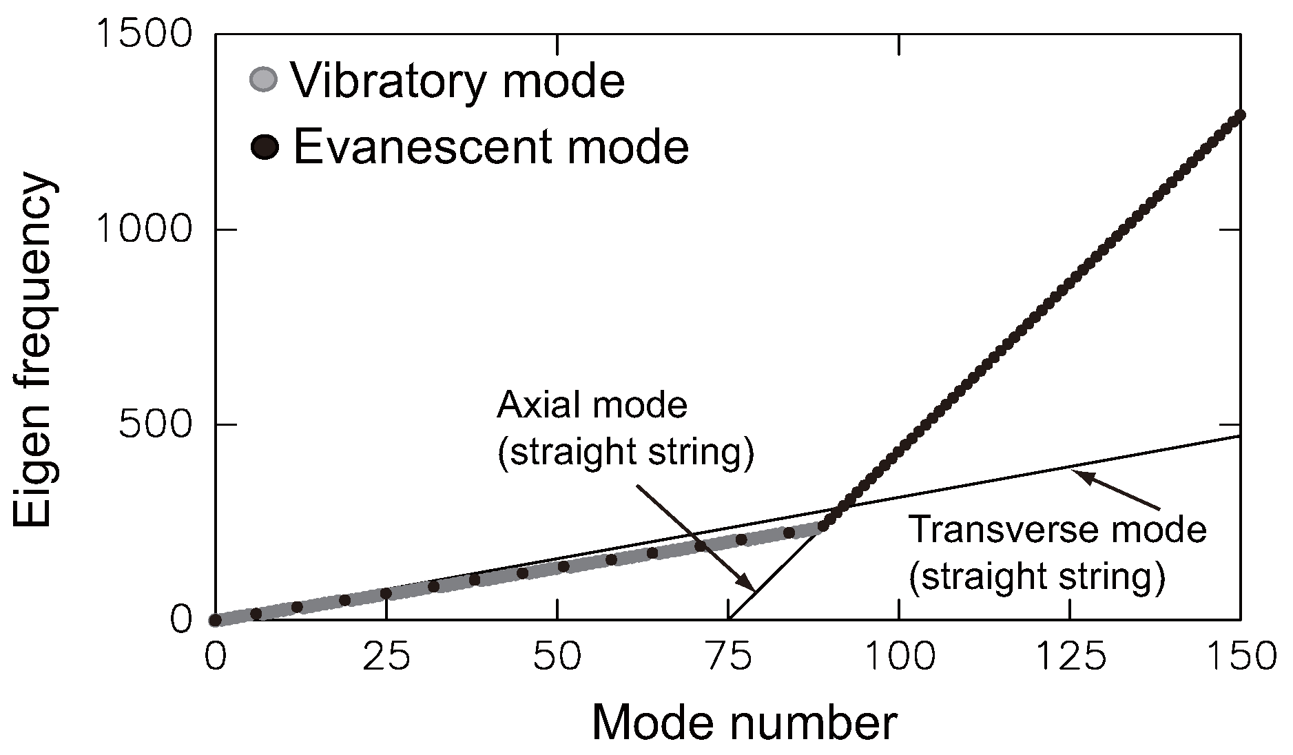
The numerical convergence of the solutions produced by the mode expansion method is verified by performing a couple of calculations with varying n.

In Figure 4, the tangential and normal components of the displacement at $t=117.5$ are plotted for $n=50$, 75, and 100. The displacements for $n=50$ differ marginally from that observed in other cases. In contrast, the calculations for $n=75$ and 100 provide similar displacement distributions. The dynamic tension and curvature exhibit sufficiently converged distributions. The short wavelength fluctuations in the distributions arise from the insufficient resolution for the short wavelength constituent of the dynamic response. On the basis of the above discussion, the result obtained using $n=75$ will be used in the following discussion.

5.3. Eigenvalues

Eigenvalues are determined by solving Equation (34) based on the properties of the cable presented in Table 1. This eigenvalue problem has $4n$ solutions, among which $2n$ ones are complex conjugates of the remaining $2n$ ones. Figure 5 denotes only the positive imaginary parts against the mode number. The mode numbers are assigned in the decreasing order of magnitude of the eigenvalues.

Figure 5 also denotes the eigenfrequency for a straight string, which are analytically given as $\omega =j\pi v_{\mathrm{c}}$ for a transverse vibration and $\omega =\left(j-n\right)\pi v_{\mathrm{l}}$ for an axial vibration (j denotes the mode number, and $\omega$ denotes the eigenfrequency), e.g., [22]. In Figure 5, the lower end of the line for axial vibration is placed at $(j,\omega )=(n,0)$ to count the mode number of axial vibration from $n+1$.

The eigenfrequencies of the curved cable are categorized into two groups; the first is mostly proportional to the line $\omega =j\pi v_{\mathrm{c}}$, whereas the second is on the line $\omega =\left(j-n\right)\pi v_{\mathrm{l}}$. The eigenfrequencies of the vibratory mode of the curved cable are close to those for the transverse mode of the straight string. It should be noted that they disagree based on the presence of a curvature. The second group comprises axial vibration modes, all of which are evanescent and immediately disappear after they are excited.

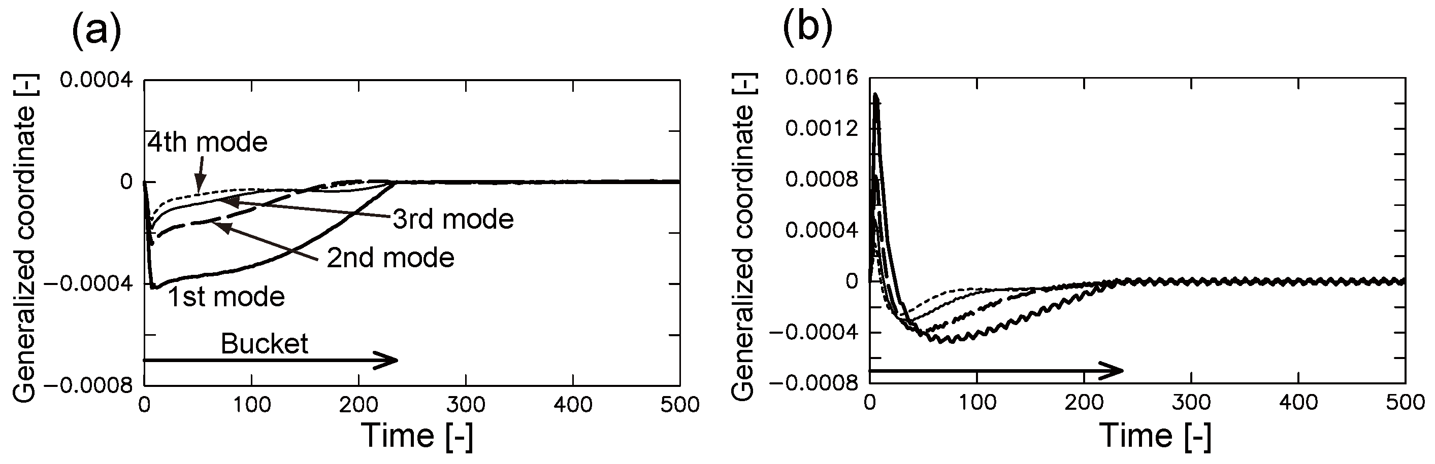
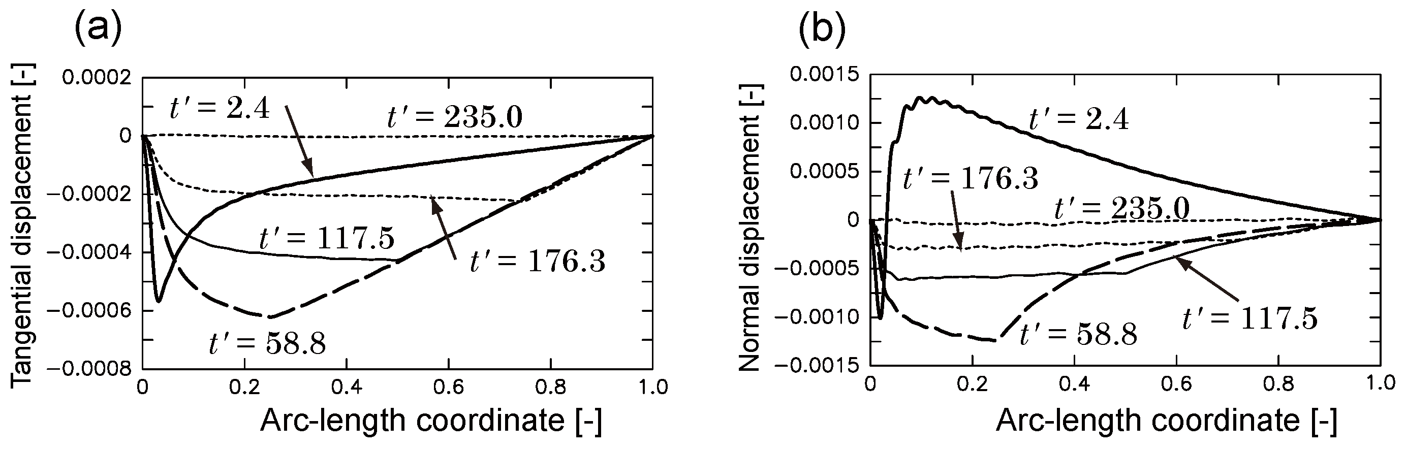
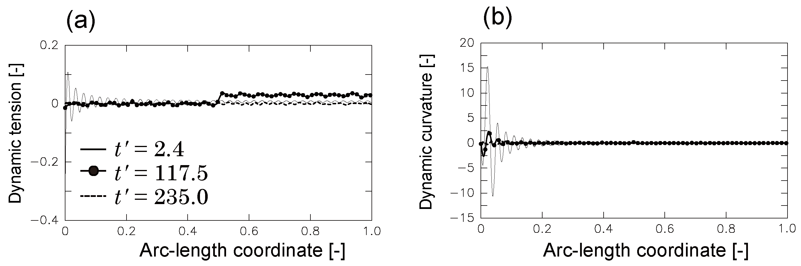
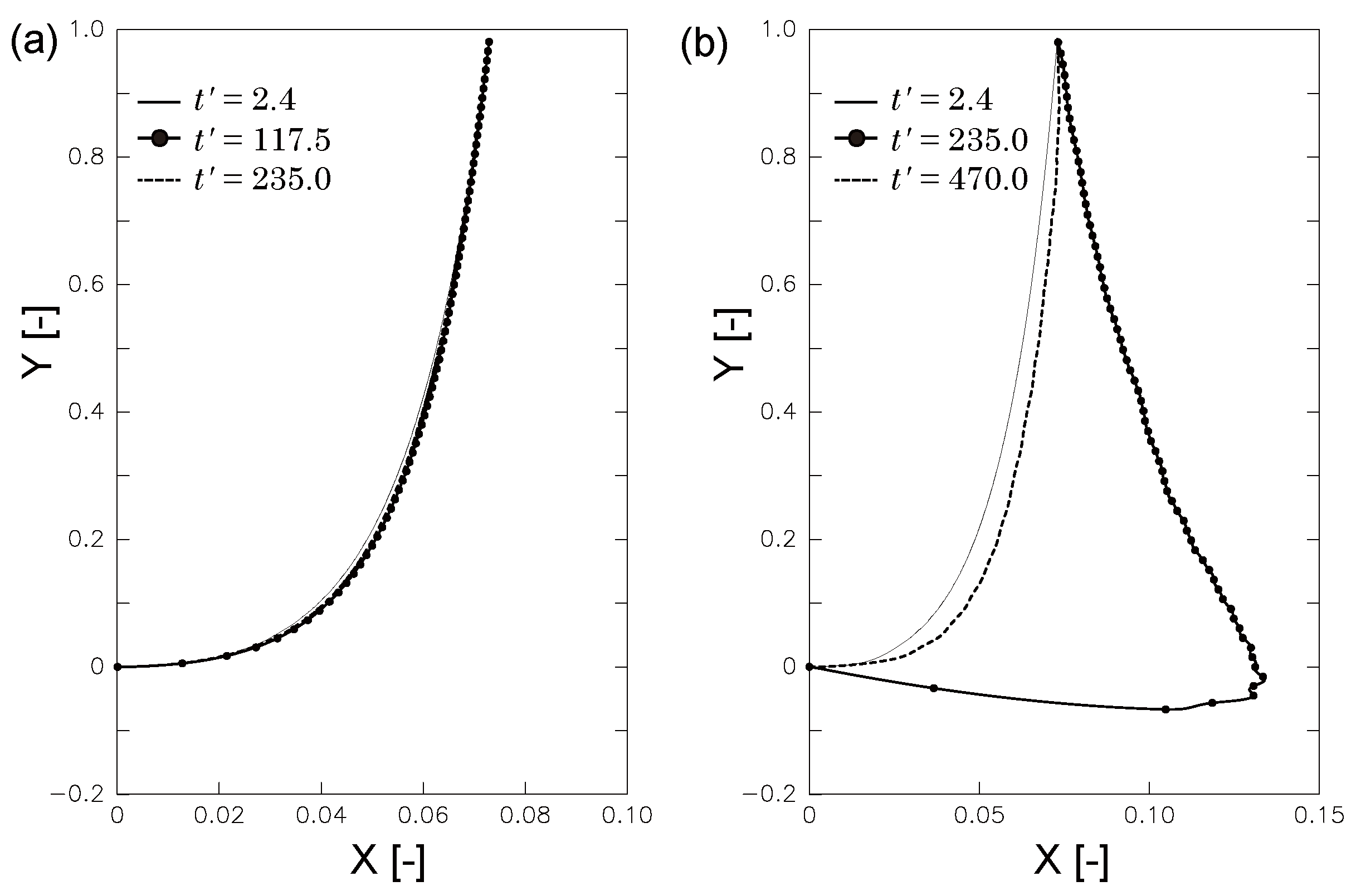
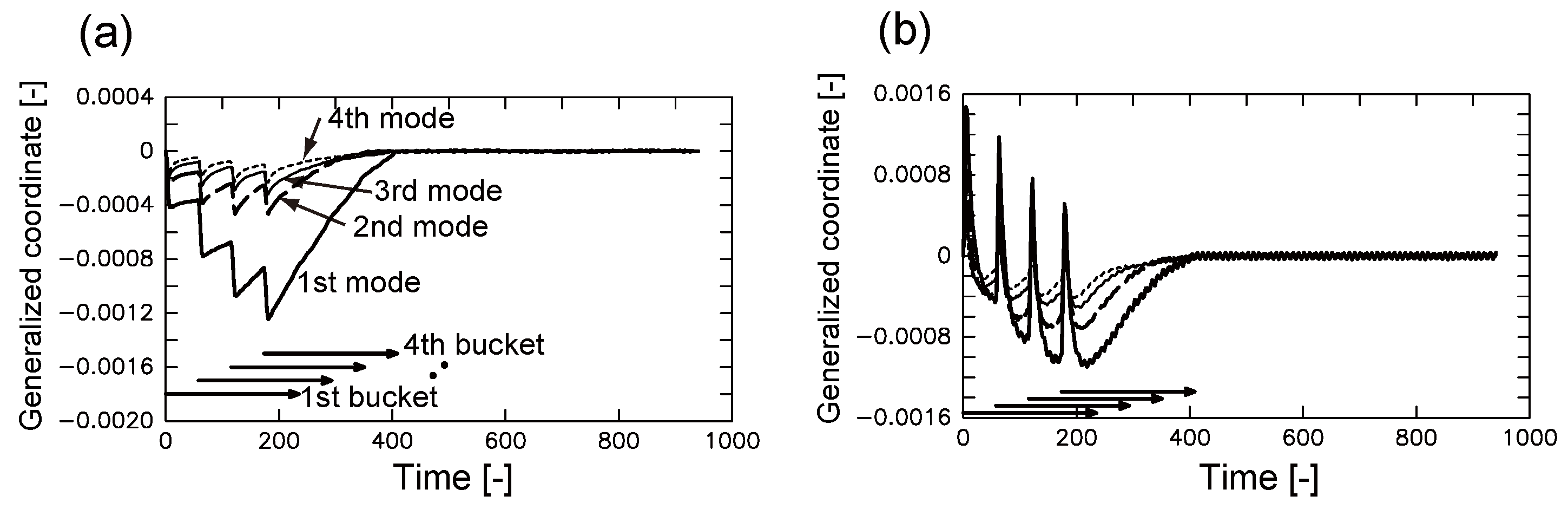
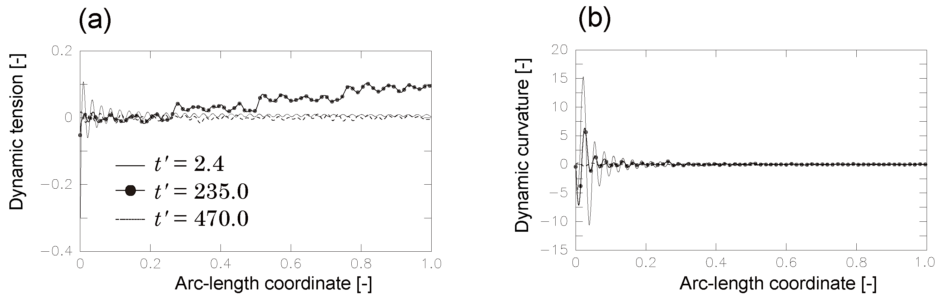
5.4. Response to Moving Load

5.4.1. One Bucket Case

The response to the load of one bucket is simulated to clearly demonstrate the effect of a single bucket. The starting point of the bucket is assumed to be at the lower end, $s_1^0=0$. Figure 6 depicts the temporal changes in the generalized coordinates of the lowest four modes. First, a transient response can be observed while lifting a bucket from the bottom to the top end, and it subsequently transforms into vibration response when the bucket passes at the top end.

The spatial distribution of the displacements exhibits a deformation of the cable caused by the load of the bucket (Figure 7). The distributions are the sharpest at the point at which the bucket is located. The normal displacement becomes smaller as time passes because the load is pointed downward as the bucket moves upward on the catenary path.

The dynamic tension indicates that the disturbance excited at the bottom end quickly travels toward the top end (Figure 8). The passage of the bucket disturbs the tension; however, the disturbance quickly decays because of hydrodynamic damping. The curvature begins to respond near the bottom end, and its disturbance propagates in the same manner as the disturbance of the tension (Figure 8).

The configuration of the cable in the X–Y coordinate system is depicted in Figure 9a. The deflection due to the bucket load is distinct immediately after the departure of the bucket from the bottom end. This is because the normal component of the bucket load is the largest when the bucket is located near the bottom end. After the bucket passes over the top, the cable is released from the load, vibrating around the static configuration with considerably small amplitudes.

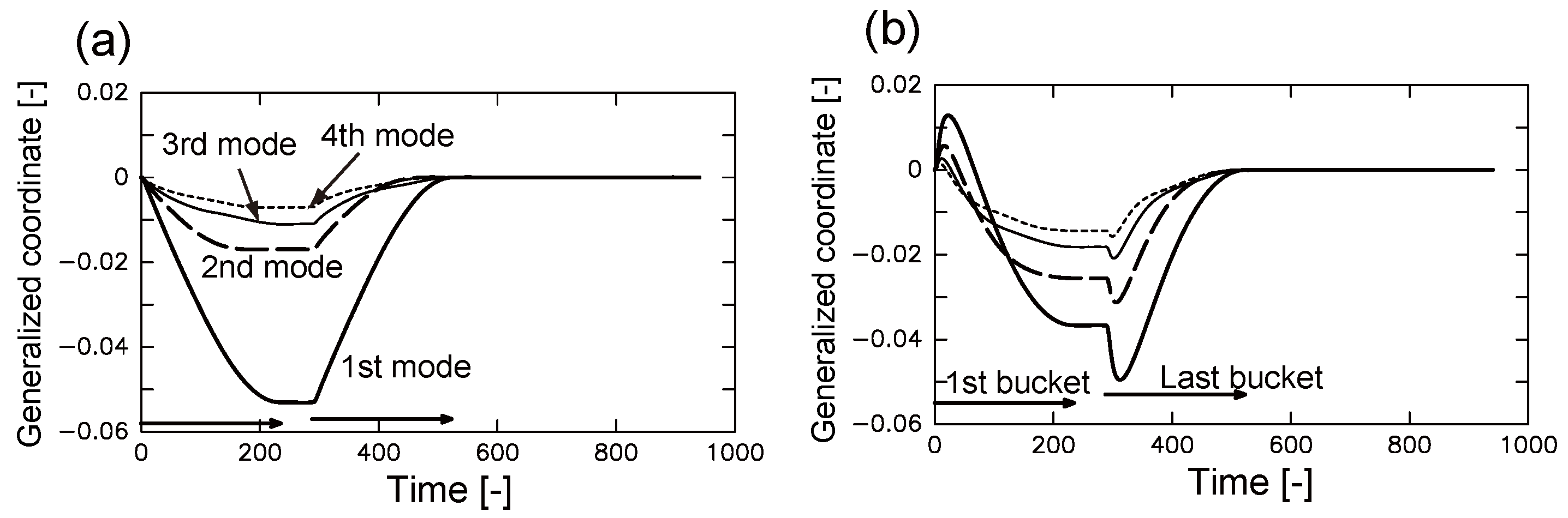
5.4.2. Four Buckets Case

Next, four buckets are incorporated into the calculation to examine the effect of a load from multiple buckets on the cable response. The load of the four buckets consecutively provides disturbances to the cable and then ceases after the fourth buckets passes the top end, where the cable is restored to the static position (Figure 10). Figure 11 depicts that the displacement becomes large in the lower part of the cable as a new bucket departs, whereas the displacement decreases when the fourth bucket approaches the top end.

The dynamic tension demonstrates a stepwise increase (Figure 12) and accumulates as the next bucket begins to leave the bottom end. The tension is eventually maximized around the top end. Meanwhile, the maximum curvature stays near the bottom end even after the buckets are far from it.

The configuration in the X–Y frame in this case is very similar to that for one bucket (Figure 9a).

5.4.3. 250 Buckets Case

The total number of 250 is close to that observed in the actual applications of the CLB system. The load from a large number of buckets results in a continuous response because buckets depart consecutively from the bottom end. The time histories of the generalized coordinates (Figure 13) are very smooth when transient response occurs as opposed to those observed in case of one and four buckets, which exhibit a discrete response to each bucket. The absolute values of the generalized coordinates are considerably larger in this case when compared with those for the remaining two cases because the total load from 250 buckets is considerably larger, yielding a larger magnitude of displacement (Figure 14).

Furthermore, the accumulation of dynamic tension toward the top end is observed in this case (Figure 15). A large number of moving buckets increases the tension toward the top; however, the increase is not stepwise but almost linear, indicating that the discreteness of the response is no longer clear and that the load of buckets is temporally continuous during the evolution of tension.

5.4.4. Relation of In-Plane Deflection and the Design of CLB

The curvature exhibits its maximum magnitude only near the bottom (Figure 15b). In the three aforementioned cases, the dynamic curvature is observed to be locally large near the bottom end. This stems from the fact that the catenary curve is almost horizontal in proximity to the bottom end, where the load of buckets mainly deflects the cable. This aspect is of prime importance while designing an axially moving catenary cable.

The cable configuration in the X–Y frame (Figure 9b) sags to a greater extent when compared with those for a smaller number of buckets (Figure 9a,b). A large sag leads to a large deviation of the bucket paths from the catenary curve in the static state, and it may reduce the number of resources that can be scooped by the buckets and that can alter the cable circulation stability in the CLB system. Hence, the sag should be considered to be an important design parameter.

The limitations of this study are as follows. First, this calculation permits the lower part of the cable to sink below the $Y=0$ line for a case involving 250 buckets. This unrealistic behavior may be eliminated by imposing surface normal forces on the part in contact with the floor.

Second, there is room for arguments, especially regarding the boundary condition at the bottom end. Another type, such as the free-end condition, may be appropriate because the cable is not fixed at the touchdown point in the actual CLB system. This issue can be tackled by developing a dynamic model capable of considering the grounded part of the cable as well as the suspended part. If the vicinity of the touchdown point has to be examined, the bending rigidity of the cable should be included in the equations. The theory presented in this study can be extended to achieve this.

The next step of the analysis for the static and dynamic responses must consider uncertainties in the responses, because the external loads on the cable involve considerable irregularities. This condition is similar to ones for bridge [23] and wharf [24], which deform and vibrate due to wind and wave loads, respectively. Evaluations of the response uncertainty and structural reliability for the cable can be achieved by constructing a stochastic model of the cable mechanics. The present deterministic model can provide a basis for the stochastic model.

6. Conclusions

This study examined the static and dynamic responses of the underwater axially moving cables to loads of the buckets attached to the cables. In particular, the in-plane deflection of the cable is analyzed through linear analyses. The equations that govern the dynamic response of the cable were solved by adopting the mode expansion method.

The calculations using different maximum numbers of mode expansion confirmed the convergence of numerical computation. The comparison between the numerical and analytical integrations demonstrated that the implemented numerical scheme can precisely compute the convolution integrals involved in the expression of a solution.

Several simulations were performed by varying the total number of buckets. According to the simulation results, the cable transiently responds to the bucket load and exhibits a vibratory variation when the cable is released from the load. The load of each bucket discretely disturbs the cable if only a few numbers of buckets are attached. As the total number of buckets increases, the load becomes spatially continuous and the response magnitude increases, producing a deviation in the trajectory of the buckets from the catenary curve observed in the static state.

References

1. Chen, L.Q. Analysis and control of transverse vibrations of axially moving strings. Appl. Mech. Rev. 2005, 58, 91–116. [Google Scholar] [CrossRef]
2. Chung, J.S. Deep-ocean mining technology: Development II. In Proceedings of the Sixth ISOPE Ocean Mining Symposium, Changsha, China, 9–13 October 2005. [Google Scholar]
3. Masuda, Y.; Mero, J.L.; Cruickshank, M. Continuous bucket line dredging at 12,000 feet. In Proceedings of the Offshore Technology Conference, Houston, TX, USA, 19–21 April 1971; pp. 837–858. [Google Scholar]
4. Masuda, Y.; Cruickshank, M.J. Mechanical design developments for a CLB mining system. In Proceedings of the Ocean Technologies and Opportunities in the Pacific for the 90’s (OCEANS’91), Honolulu, HI, USA, 1–3 October 1991; pp. 1583–1586. [Google Scholar]
5. Jones, N.P.; Scanlan, R.H. Theory and full-bridge modeling of wind response of cable-supported bridges. J. Bridge Eng. 2001, 6, 365–375. [Google Scholar] [CrossRef]
6. Rizzo, F.; Caracoglia, L.; Montelpare, S. Predicting the flutter speed of a pedestrian suspension bridge through examination of laboratory experimental errors. Eng. Struct. 2018, 172, 589–613. [Google Scholar] [CrossRef]
7. Simpson, A. On the oscillatory motions of translating elastic cables. J. Sound Vib. 1972, 20, 177–189. [Google Scholar] [CrossRef]
8. Triantafyllou, M.S. The dynamics of translating cables. J. Sound Vib. 1985, 103, 171–182. [Google Scholar] [CrossRef]
9. Perkins, N.C.; Mote, C.D., Jr. Three-dimensional vibration of travelling elastic cables. J. Sound Vib. 1987, 114, 325–340. [Google Scholar] [CrossRef]
10. Nishi, Y. Static analysis of axially moving cables applied for mining nodules on the deep sea floor. App. Ocean Res. 2012, 34, 45–51. [Google Scholar] [CrossRef]
11. Nishi, Y. Determining the grounding length of an axially moving cable in a two-ship continuous line bucket system. Appl. Ocean Res. 2013, 40, 42–49. [Google Scholar] [CrossRef]
12. Nishi, Y.; Yamai, T.; Ikeda, K. Two-belt continuous line bucket system: Its concept design and fundamental bucket motion experiments. Appl. Ocean Res. 2015, 53, 125–131. [Google Scholar] [CrossRef]
13. Wickert, J.A.; Mote, C.D., Jr. Classical vibration analysis of axially moving continua. J. Appl. Mech. 1990, 57, 738–744. [Google Scholar] [CrossRef]
14. Meirovitch, L. A new method of solution of the eigenvalue problem for gyroscopic systems. AIAA J. 1974, 12, 1337–1342. [Google Scholar] [CrossRef]
15. Meirovitch, L. A modal analysis for the response of linear gyroscopic systems. J. Appl. Mech. 1975, 42, 446–450. [Google Scholar] [CrossRef]
16. Swope, R.D.; Ames, W.F. Vibrations of moving threadline. J. Frankl. Inst. 1963, 275, 36–55. [Google Scholar] [CrossRef]
17. Hildebr, F.B. Advanced Calculus for Applications, 2nd ed.; Prentice-Hall Inc.: Upper Saddle River, NJ, USA, 1976. [Google Scholar]
18. Bliek, A. Dynamic Analysis of Single Span Cables. Ph.D. Thesis, Massachusetts Institute of Technology, Cambridge, MA, USA, 1992. [Google Scholar]
19. Wilson, J.F. Dynamics of Offshore Structures, 2nd ed.; John Wiley&Sons Inc.: Hoboken, NJ, USA, 2002. [Google Scholar]
20. Boas, M.L. Mathematical Methods in the Physical Sciences, 3rd ed.; John Wiley&Sons Inc.: Hoboken, NJ, USA, 2004. [Google Scholar]
21. Zibdeh, H.S.; Rackwitz, R. Moving loads of beams with general boundary conditions. J. Sound Vib. 1996, 195, 85–102. [Google Scholar] [CrossRef]
22. Meirovitch, L. Elements of Vibration Analysis, 2nd ed.; McGraw-Hill Inc.: New York, NY, USA, 1986. [Google Scholar]
23. Canor, T.; Caracoglia, L.; Denoël, V. Application of random eigenvalue analysis to assess bridge flutter probability. J. Wind Eng. Ind. Aerod. 2015, 140, 79–86. [Google Scholar] [CrossRef] [Green Version]
24. Schoefs, F.; Yáñz-Godoy, H.; Lanata, F. Polynomial chaos representation for identification of mechanical characteristics of instrumented structures. Comput-Aided Civ. Inf. Eng. 2011, 26, 173–189. [Google Scholar] [CrossRef]
Figure 1. Schematic of a two-ship continuous line bucket (CLB) system. The circular cable comprises two suspended parts (ascending and descending parts) and a grounded part. The dashed box represents the ascending part addressed in this study.
Jmse 07 00301 g001
Figure 2. O X Y Cartesian and arc-length (s) coordinate systems. The dashed box enlarges a point on the cable to denote the definition of angles and displacements.
Jmse 07 00301 g002
Figure 3. Comparison of the computed results using analytical and numerical integrations for a straight cable: (a) tangential displacements; and (b) normal displacements at t = 117.5 .
Jmse 07 00301 g003
Figure 4. Convergence of the computed results using three maximum numbers of mode expansion, n = 50 , 75, and 100: (a) tangential displacement; (b) normal displacement; (c) dynamic tension; and (d) dynamic angle.
Jmse 07 00301 g004
Figure 5. Plots of the eigenfrequencies (imaginary part of the eigenvalue) against the mode numbers. The lines represent the eigenfrequencies of the axial and transverse vibrations of a straight string.
Jmse 07 00301 g005
Figure 6. Temporal changes in the generalized coordinates of the lowest four modes for one bucket: (a) tangential component and (b) normal component.
Jmse 07 00301 g006
Figure 7. Distributions of the (a) tangential and (b) normal displacements for one bucket. t denotes dimensionless time.
Jmse 07 00301 g007
Figure 8. Distributions of the (a) dynamic tension and (b) dynamic curvature for one bucket. t denotes dimensionless time.
Jmse 07 00301 g008
Figure 9. Cable configurations in the X–Y plane for (a) one bucket, and (b) 250 buckets. t denotes dimensionless time.
Jmse 07 00301 g009
Figure 10. Time histories for the generalized coordinates of the lowest four modes in case of four buckets: (a) tangential component and (b) normal component.
Jmse 07 00301 g010
Figure 11. Distributions of the (a) tangential and (b) normal displacements for four buckets. t denotes dimensionless time.
Jmse 07 00301 g011
Figure 12. Distributions of (a) dynamic tension and (b) dynamic curvature for four buckets. t denotes dimensionless time.
Jmse 07 00301 g012
Figure 13. Time histories for the generalized coordinates of the lowest four modes for 250 buckets: (a) tangential component and (b) normal component.
Jmse 07 00301 g013
Figure 14. Distributions of the (a) tangential and (b) normal displacements for 250 buckets. t denotes dimensionless time.
Jmse 07 00301 g014
Figure 15. Distributions of the (a) dynamic tension and (b) dynamic curvature for 250 buckets. t denotes dimensionless time.
Jmse 07 00301 g015