On the Information Advantage of Sidescan Sonar Three-Frequency Colour over Greyscale Imagery

Abstract

A prototype three-frequency (114, 256, and 410 kHz) colour sidescan sonar system, built by Kongsberg Underwater Mapping Ltd. (Great Yarmouth, UK), was previously described, and preliminary results presented, in Tamsett, McIlvenny, and Watts. The prototype system has subsequently been modified, and in 2017, new data were acquired in a resurvey of the Inner Sound of the Pentland Firth, North Scotland. An image texture characterisation and image classification exercise demonstrates considerably greater discrimination between different seabed classes in a three-frequency colour sonar image of the seabed, than in a multi-frequency colour image reduced to greyscale display, or in a single-frequency greyscale image, with readily twice the number of classes of seabed discriminated between, in the colour image. The information advantage of colour acoustic imagery over greyscale acoustic imagery is analogous to the information advantage of colour television images over black-and-white television images. A three-frequency colour sonar image contains a theoretical maximum of a factor of 3 times the information in a corresponding greyscale image, for independent seabed responses at the three frequencies. Estimates of the average information per pixel (information entropy) in the colour image, and in corresponding greyscale images, reveal an actual information advantage of colour sonar imagery over greyscale, to be in practice approximately a factor of 2.5, empirically confirming the greater information based utility of three-frequency colour sonar over greyscale sonar. Reference: Tamsett, D.; McIlvenny, J.; Watts, A. J. Mar. Sci. Eng. 2016, 4(26).

1. Introduction

Multi-frequency acoustic colour imagery is not a new idea, and along with multi-frequency radar colour imagery, was patented a surprisingly long time ago [1]. However, until recently there had been no practical realisation and implementation of colour sonar. For acoustic colour to be a meaningful property of the seabed, acoustic backscatter amplitude as a function of frequency must be reduced to an effect of the seabed alone, un-conflated by other effects. Otherwise, conflation leads to colour having a psychedelic effect on the mind, deleterious to interpretation of the nature of the seabed. Two-frequency sidescan sonar acoustic colour images (red, blue, and grey) were generated by Tamsett [2]. Three-frequency multi-beam acoustic images are shown in Hughes Clarke and Muggah [3] and Hughes Clarke [4], and three-frequency sidescan sonar acoustic images were generated by Tamsett and McIlvenny [5], Tamsett, McIlvenny, and Watts [6], and McIlvenny et al. [7]. There have recently been other investigations incorporating multi-frequency sonar, some including colour imagery [8,9,10,11]. These contributions have qualitatively demonstrated an advantage of multi-frequency colour over greyscale sidescan sonar imagery.

A description of a prototype three-frequency colour range-only sidescan sonar system built by Kongsberg Underwater Mapping Ltd. (Great Yarmouth, UK), and preliminary results acquired in 2015, are presented in Tamsett et al. [6] and Tamsett, McIlvenny, and King [12].

A summary description of the system hardware follows: The system pings simultaneously at three frequencies: 114, 256, and 410 kHz. The pings are 16 cycles; 128, 64, and 32 microseconds long, with fore-aft sonar beam widths; 1.0°, 0.75°, and 0.5°. The beams were originally directed at an inclination of 20° below the horizontal [6,12]. The sonar fish incorporates an attitude sensor for measuring pitch, roll, and heading. In the earlier system, the measurement of heading was subject to large systematic and random error and was inadequately poor. The sonar fish has hitherto generally been pole-mounted, and in this way coupled to the side of the research vessel. A GPS (Global Positioning System) measures geo-position and vessel heading.

In a colour sonar system, data processing is particularly important. A geometrical spreading correction is applied. During data acquisition, a time varied gain of +30logR decibels (where R is one-way travel range) is applied. The effect of the area of seabed ensonified by the sonar pulse, as a function of range and inclination angle, is accounted for more accurately post-acquisition [13]. A correction for absorption is applied (+2RA decibels, where A represents the respective absorption coefficients for the three carrier wave frequencies: 0.0335, 0.0600, and 0.1007 decibels/meter [14]). To account for the angular response of the sonar in the vertical plane orthogonal to the axis of sonar fish, and the angular response of the seabed as a function of grazing angle, a process of trace normalisation is applied [15,16].

Attempts to acquire new data in 2016 were frustrated by an impediment in the system hardware, affecting data acquired using a pole mounting of the sonar fish. The near sea surface deployment of a pole-mounted sonar fish meant the 20° inclination of the transducers’ faces was insufficiently steep for the large angular extent of sonar’s acoustic pulses in the vertical plane, particularly at the higher frequencies. Even in moderate sea states, backscatter from a disturbed sea surface, exacerbated by sonar vehicle roll, produced a deleterious effect, sometimes severely so, on data quality. To mitigate the problem, 15° wedges have been inserted between the transducers’ housing and the sonar fish frame to increase the inclination of the transducers’ faces to 35°.

A new and considerably improved attitude sensor card provided by Kongsberg Underwater Mapping (Great Yarmouth, UK) replaced the previous one, which had inadequately measured sonar fish heading. This replacement proved invaluable in the surveys in 2017 providing essential data supplementary to the heading data from the differential antenna in the ERI’s (Environmental Research Institute) GPS system.

In Section 2 of this paper, an image texture characterisation and sonar image classification exercise are performed on three classes of image: three-frequency colour; three-frequency data reduced to greyscale; and mid-frequency greyscale. It is shown by demonstration that there is, in practice, considerably greater discrimination between different seabed classes (types) in colour imagery, than in either of the greyscale imageries.

In Section 3, it is inferred from a consideration of basic Information Theory that there is a maximum of three times the information in a colour sonar image than in a corresponding greyscale one (howsoever it is generated), for independent data at the three frequencies. This requires that the carrier wave frequencies be sufficiently separated for independent seabed responses. An estimate of the actual information advantage achieved using our system, with a frequency span of two octaves, is made from computations of information entropy in the various images. The use and potential advantage of chirp technology for colour sonar data acquisition is discussed. It is suggested that a simple three-‘ping’-based technology, with three frequencies spanning approximately two octaves, is for the time being a practical solution to three frequency acoustic imagery of the seabed, until multi-frequency ‘chirp’-based colour sonar technology becomes available.

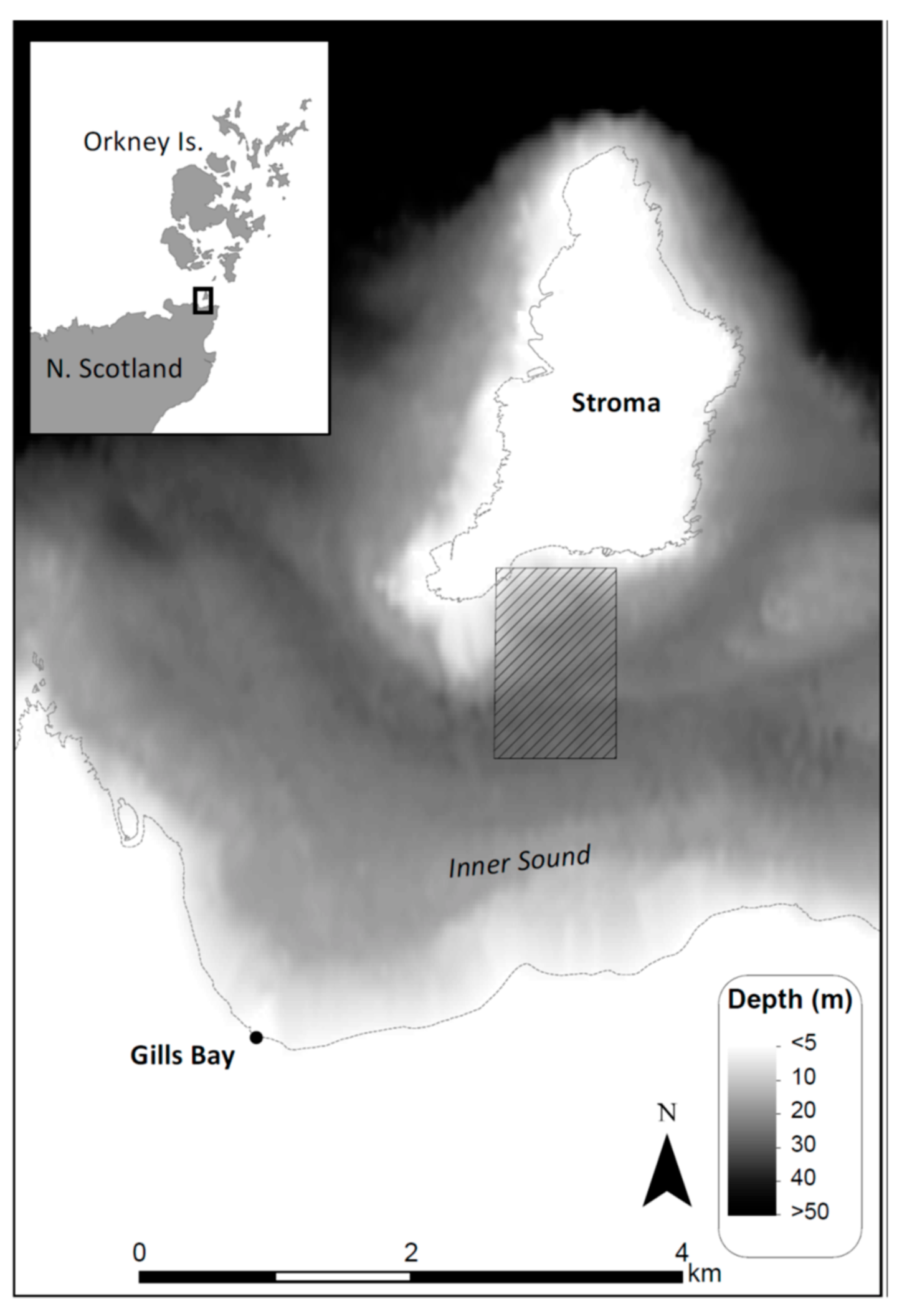
2. Resurvey of the Inner Sound, Pentland Firth

A resurvey of the Inner Sound of the Pentland Firth was carried out on 8 September 2017 (Figure 1) comprising 15 swaths running principally south to north. The swaths are shown in this paper overlain from west to east to form montages for which the direction of ensonification is therefore to the west, except along the eastern half of the easternmost swath.

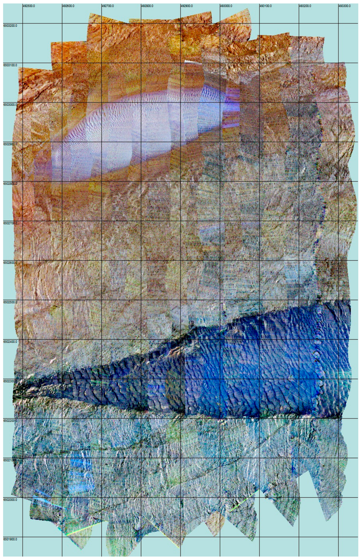
2.1. Three-Frequency Colour

A montage of three-frequency swath data generated at a resolution of 1 metre is shown as a colour image in Figure 2. Colour was generated using the ‘negative BGR’ colour scheme described in detail in Tamsett, McIlvenny, and Watts [6]. The image is ‘frequency equalized’ [6] with respect to itself. Figure 2 is very similar to images generated from data acquired for the same area during earlier surveys in 2015 [6,7]. Based on previous seabed sampling programs, and visible-spectrum subsea video camera surveys; the seabed is an exposure of Devonian flagstone (old red sandstone) dipping to the east, with a ridge of fine gravel composed of broken shell fragments running across the southern half of the survey area. In the northern half of the survey area, there is a dune of medium sand overlying, and surrounded by, a bed of small smooth cobbles. The seabed exposures of Devonian flagstone rock appear as a wide variety of shades of coloured image texture varying in colour from shades of violet and blue to shades of reddish brown. This wide variety in acoustic colour is currently not explained in terms of more direct ground truth observation of the seabed, for example by sub-aqua diving, or by near seabed photography, or video.

The gravel ridge across the southern half of the survey area strongly backscatters, particularly the high-frequency sonar signal, and appears as a variety of shades of blue. Due to a constraint on the time available to conduct the survey, swaths were acquired initially from east to west, but are mixed with others acquired later in the day from west to east. The lateral contrasts in the shades of blue across vertical boundary lines evident along the gravel ridge in the montage are not an artefact but are in fact real, evidenced by the absence of similar corresponding contrasts associated with the rock exposure north and south of the gravel ridge. The contrast along the gravel ridge arises due to the change in the backscattering characteristics of the gravel through the tidal cycle. This is a point of interest, and it is a future intention to conduct a detailed investigation of the anisotropic nature of backscattering from the material comprising the gravel ridge, and how it changes through the tidal cycle. The cobble bed in the northern half of the survey area strongly backscatters particularly the low-frequency sonar signal and appears as dark shades of hazel brown. The sand dune overlying the cobble bed weakly backscatters signal at all sonar frequencies especially the lower frequencies and it appears on the montage as shades of light blue. Whilst the presence and distribution of the gravel and sand sediments in the survey area are well understood in terms of the tidal dynamics [7], the presence of the cobble bed underlying the sand dune is not yet adequately understood or explained.

Comparison of the image in Figure 2 for data acquired in September 2017, with an image generated for data acquired in 2015 in similar sea states [6], reveals that the detrimental effect of backscattering from the sea surface is considerably less in the recently acquired data. Thus, the effect of the 15° wedges placed behind the sonar’s transducers is a positive one, successfully mitigating backscatter from the sea surface. The problem is not completely eradicated however, and where highest quality data are required, particularly in higher sea states, it will probably be necessary to resort to towing the sonar fish rather than employing pole mounting. This will allow the sonar fish to fly deeper in the water column and decouple the fish from research vessel roll. Towing does incur the disadvantage of reducing geo-positional accuracy in swath montages and can lead to problems with snatching in higher sea states. It also places a restriction on close access to coastlines, and makes avoiding lobster pot lines and other hazards more difficult. In all but mill-pond conditions, towing rather than pole mounting may be required with this system as currently constituted to maximize data quality. The new attitude sensor in the prototype system has greatly improved measurement of sonar fish heading, making towing rather than pole-mounting a feasible option.

A user-supervised texture-mapped image of the three-frequency colour sonar image is shown in Figure 3. This was generated using GeoTexture sonar data and image processing software (Kongsberg Underwater Mapping Ltd., Great Yarmouth, UK). An iterative two-stage user-supervised process was employed to generate the texture-mapped image [17]. First, a small area of seabed image texture (typically roughly 10 by 10 pixels; ~100 pixels in all) is selected, and the image texture characterised by extracting features from the images at each of the selected pixels, and computing statistics describing the way the features, are distributed in feature space. Second, a classification process is applied to the whole image. Features extracted at every pixel are matched against the texture characteristics in a collection of seabed image texture characteristics and classified according to the seabed class that best matches. In the absence of a close match (determined by setting a decision threshold—a distance in ‘standard deviations’), a pixel is explicitly classified as unrecognised. Subsequently, an area of unrecognized image texture in the classified image that ensues is selected for characterisation in the manner already described, and the whole image re-classified. This iterative process is continued until the image texture characterisation process is completed.

The advantage of the user-supervised approach over an unsupervised one is that where selection of areas of seabed for image texture characterisation is supported by ground-truth information (not applicable in this study), the texture-mapped image constitutes an interpretation otherwise the texture-mapped image represents merely a segmented image.

The characterisation and classification processes are based on ‘features’ extracted from the backscatter image at each pixel. Three features are extracted from data in the vicinity of a pixel, as a function of frequency (i.e., three features per frequency, nine in all, at each pixel). Features at a pixel were extracted from data within a circular window on the image 17 pixels in diameter. Feature 1 is the backscatter value that emerges after applying a low-pass (LP) filter, nine (1 + 17/2) pixels across, to the backscatter image. Feature 2 is a measure of the energy in the image removed in applying the LP filter nine pixels across, to the backscatter data. Feature 3 is a measure of the additional energy removed in applying an LP filter 17 pixels across to the data. The values for energy removed at each pixel are themselves also LP filtered with a filter nine pixels across. Features 2 and 3 provide multi-scale measures of image texture. Image texture characteristics for the small area of seabed selected by the user are computed from the three features in a three-dimensional feature space for data at each of the three frequencies. In applying a process of texture classification to a pixel in an image, the three features for the data at each frequency are extracted and a ‘distance’ (in standard deviations) determined between the pixel’s position in feature space and each class of image texture for which characteristics are extant. The measure of distance in ‘standard deviations’ (SDs) is based on statistical quantities computed from the distribution of features in feature space when a texture is characterised. A ‘distance’ between a pixel and a characterised seabed type may subsequently be expressed using the SD metric. The classification process finds the seabed class for which the ‘distance’ is a minimum. However, should this distance exceed a user-determined threshold distance (e.g., set to 5 standard deviations for the image texture characterisation process, and 12 for generating a classified image for inclusion in a report), the pixel is classified as unrecognised image texture.

The top section of

Table 1. Top: Seabed image textures selected from the three-frequency colour sonar image (Figure 2) during a user-supervised image texture characterisation process, subsequently used to generate the classified image (Figure 3). Bottom: A matrix of class separations (in standard deviations) computed for the image texture characteristics extracted from the three-frequency colour backscatter image.

shows a representation of the set of seabed image texture classes for which characteristics were extracted from the data used to generate Figure 2, and which were subsequently used to generate the classified image shown as Figure 3. Each characterised texture is associated with an enumeration (column 1), a text label providing a pithy description of the nature of the seabed (column 2), a colour used to represent the image texture in classified images (column 3), and the sonar backscatter data for the areas selected for image texture characterisation shown as small images (column 4).

Image texture characteristics were extracted from the colour sonar backscatter data used to generate Figure 2 in the order that they appear in rows from top to bottom in the top section of Table 1. They were extracted in turn and the image classified after each characterisation with the ‘decision threshold’ set to a low value (5 standard deviations) to ensure that only sufficiently disparate image textures were characterised and to avoid a conflation of indistinguishable image textures in a collection of image texture classes.

The lower section of Table 1 shows the result of running a ‘class discrimination matrix’ process in the GeoTexture software to the set of seabed image characteristics represented in the upper section of Table 1. The matrix provides a measure of ‘distance’ in standard deviations (SDs) between all pairs of image texture classes. Note that all distances are large, the smallest being 6.4 SDs, and that the distances between pairs of classes is asymmetrical. The asymmetry is analogous, for example, to the probability of misidentifying a buzzard as an eagle (relatively large) being different from the probability of misidentifying an eagle as a buzzard (very small).

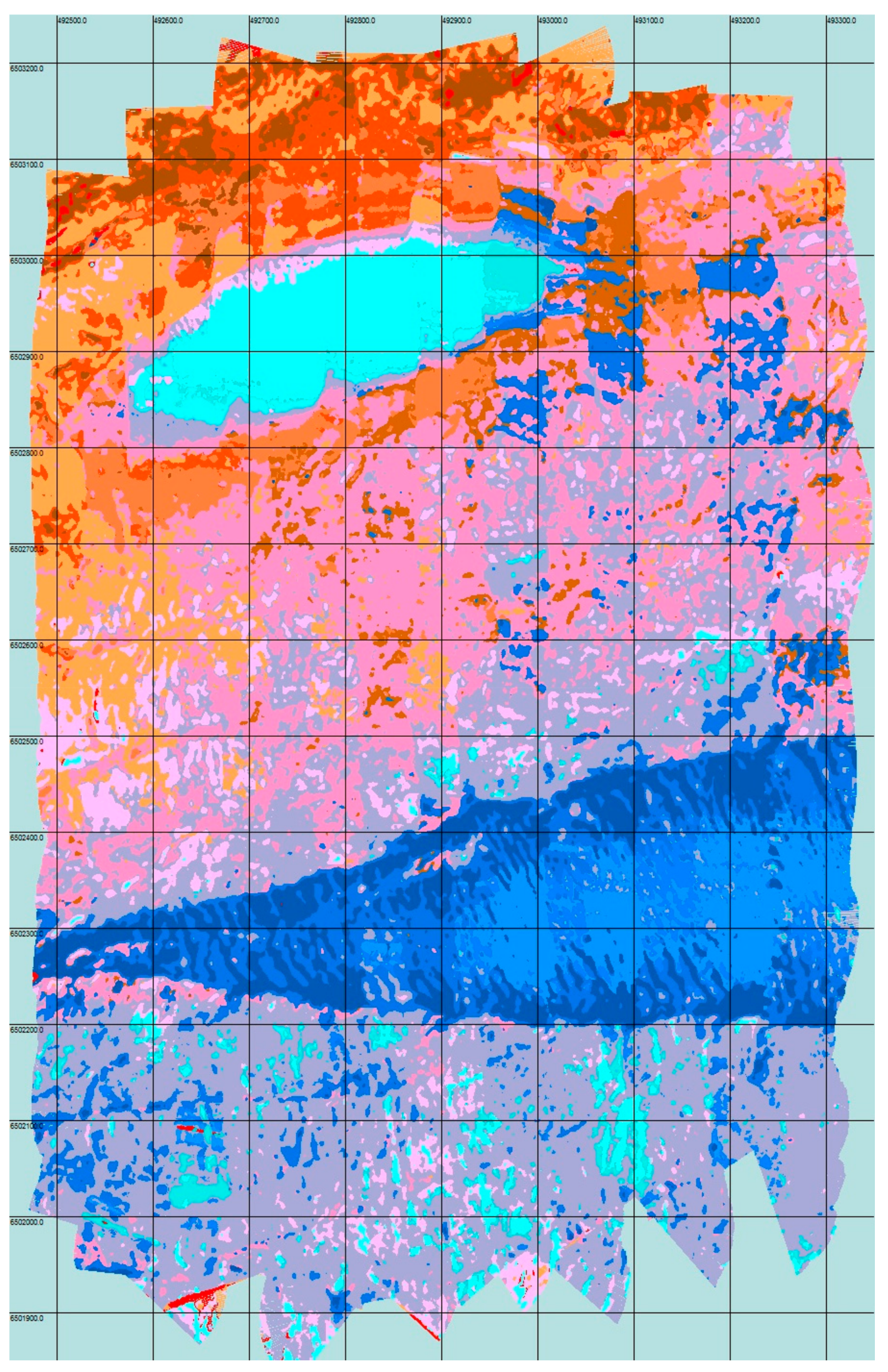
2.2. Three-Frequency Colour Reduced to Greyscale

A pair of figures and a table corresponding to Figure 2 and Figure 3 and Table 1 for the colour image already described are shown for the three-frequency colour reduced to a greyscale image in Figure 4 and Figure 5 and

Table 2. Top: Seabed image textures for the three-frequency colour reduced to greyscale sonar image selected during a user-supervised image texture characterisation process. These were subsequently used to generate the classified image (Figure 5). Bottom: A matrix of the probabilities of classifying one class as another; and a matrix of class separations (in standard deviations) computed for the image texture characteristics extracted from the colour reduced to greyscale backscatter image.

. Reduction to greyscale of the colour image was carried out by assigning to the R, G, B values for the greyscale image, the mean of the R, G, B values of the colour image. The greyscale image (corresponding to Figure 2) is shown in Figure 4.

For many people it might be thought to be self-evident that the colour image (Figure 2) contains much more information on the nature of the seabed than the greyscale one (Figure 4). This is directly analogous to most people choosing to watch colour television in preference to a black-and-white one because, quite simply, there is more information in a colour television display that in a black-and-white one, though quite likely many people may be unaware of their reason for their preference. Surprisingly however, it is not immediately obvious to everyone that a colour sonar image reveals more about the seabed than a greyscale one!

The result of a texture mapping exercise applied to Figure 4 is shown in Figure 5. The colour reduced to greyscale image seabed texture classes are represented in Table 2 (top). The areas of seabed used to extract characteristics (from Figure 4) are a subset of those used to extract colour image texture classes from the analogous colour image (Figure 2). Where, in characterising the textures in the same order as for the colour image, the image texture in an area of seabed was found to conflate with an image texture already characterised in the emerging collection of classes, it was skipped to avoid effectively characterising the same image texture more than once. This led to a smaller number of classes for the colour to greyscale seabed texture (seven) than for the colour image of the seabed (15). A comparison of the texture-mapped/classified image in Figure 5, with the texture-mapped/classified image for the colour data (Figure 3), demonstrates that there is considerably greater discrimination between seabed image textures in the colour image than in the colour reduced to greyscale image.

The result of applying the ‘class discrimination process’ to the set of image texture classes for the colour reduced to greyscale image is shown in Table 2 (bottom). In addition to the separation matrix, a probability matrix was computed and is shown. A comparison of the separation matrix in Table 2 for the greyscale data, with the separation matrix in Table 1 for the colour data, is not strictly valid because of differences in the way colour image and greyscale image texture characteristics are represented in memory, and separations are computed. The data representing greyscale texture characteristics occupy a 3D feature space, and the data for colour texture characteristics occupy three parallel 3D feature spaces. Three parallel 3D features spaces were employed to perform separation computations on colour data, rather than a single 9D feature space, which would have led to very time-consuming computations performing matrix manipulation.

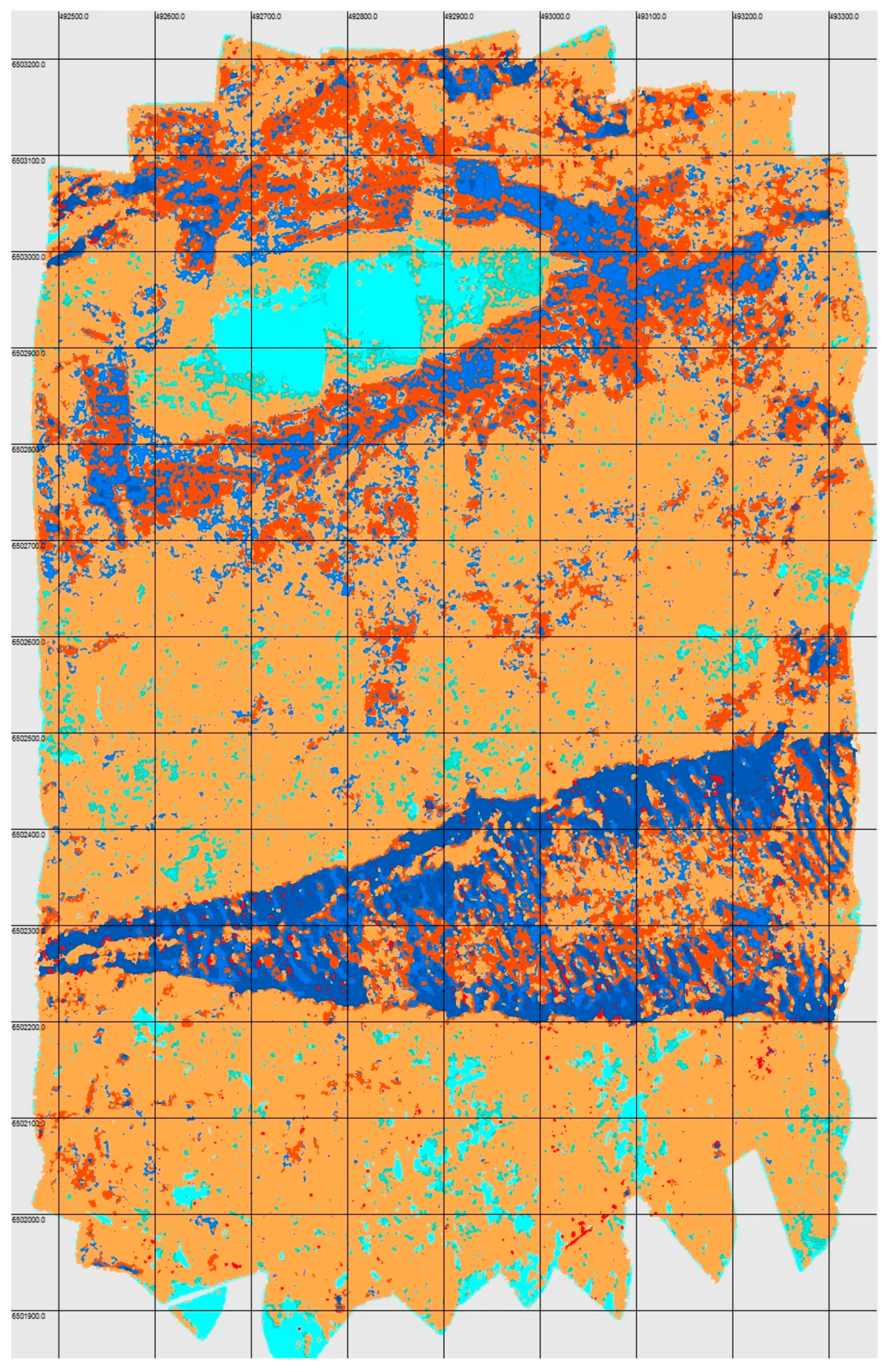
2.3. Mid-Frequency Greyscale

Finally, a set of figures and a table corresponding to Figure 2 and Figure 3 and Table 1 for the colour image, and to Figure 4 and Figure 5 and Table 2 for colour reduced to greyscale display, are shown for the mid-frequency (256 kHz) data greyscale image, in Figure 6 and Figure 7 and in

Table 3. Top: Seabed image textures for the mid-frequency greyscale sonar image selected during a user-supervised image texture characterisation process. These were subsequently used to generate the classified image (Figure 7). Bottom: A matrix of the probabilities of classifying one class as another; and a matrix of class separations (in standard deviations) computed for the image texture characteristics extracted from the mid-frequency greyscale backscatter image.

. The greyscale image (corresponding to Figure 2 and Figure 4) is shown in Figure 6.

The result generated by the texture mapping exercise applied to Figure 6 is shown in Figure 7. Arguably, the texture map generated for the mid-frequency data is a little less useful than the texture map generated for the colour reduced to greyscale image because different types of exposed rock at the seabed are not as well discriminated between; however, differences in how useful the texture maps are, for the two greyscale images, is marginal. The seabed characteristics extracted are represented in Table 3 (top). The areas of seabed used to extract image characteristics from the single frequency greyscale image are a sub-set of those used to extract characteristics from the three-frequency acoustic colour image. The number of classes of seabed image texture that emerged for the mid-frequency greyscale image is eight (compared to seven for the colour to greyscale image, and fifteen for the colour image). No significance should be attached to the apparent very marginally better image texture discrimination in the colour-to-greyscale texture map than in the mid-frequency greyscale image. A small difference like this, in a process requiring a degree of subjectivity on the part of the user, is likely to be attributable to chance. An examination of the texture map/classified image in Figure 7 again demonstrates a considerable diminution in discrimination between seabed types in the single mid-frequency greyscale image, compared to that for the three-frequency colour image.

The result of applying the ‘class discrimination process’ to the set of seabed texture characteristics for the mid-frequency greyscale image is shown in Table 3 (bottom). This table is directly comparable to Table 2. The probabilities and the separations that emerge for both tables are similar, and no significance can be attached to the relatively minor differences that might arguably be apparent in the tables. It is perhaps a little surprising that the number of distinct image texture classes, and the ability to discriminate between different types of seabed, that has emerged from the analysis of the single mid-frequency greyscale image, is approximately equal to the number that emerged for the colour reduced to greyscale image. A distinct advantage in colour reduced to greyscale over single (mid) frequency greyscale imagery might have been anticipated, but the evidence that has emerged, and is presented here, suggests that any differences are marginal. It is very likely that any minor differences in the ability to distinguish between different seabed types in the two kinds of greyscale imagery are either not, or else only marginally, significant, i.e., can be attributed to chance from the way the areas of seabed were selected for the seabed characterisation process.

3. Remarks

3.1. The Information Inherent in Colour and Greyscale Images

The quantity of information inherent in an event is:

$$I=-\log p$$

(1)

where $p$, is the probability of the event; and information, $I$, has the unit, bits, when the logarithm function applied is base $2$ (e.g., [18]).

The simplest computation for the information inherent in a greyscale image yields the unsurprising result of, 8 bits/pixel and for a colour image, 24 bits/pixel. In transmitting or encoding an image one pixel at a time in sequence, a pixel’s value can to some extent be predicted from the values of the neighbouring pixels already transmitted or encoded. The conditional probability of a pixel’s value that ensues is elevated compared to values not subject to conditional probability. The information in a pixel will, therefore, usually be somewhat less than 8 or 24 bits/pixel. In the limit, a single valued image in which all pixels have the same value, will contain 8 bits/image for a greyscale image and 24 bits/image for a colour one. The principal point here being that the information inherent in a colour image would appear to be a factor of 3 times that in the same image reduced to greyscale.

However, the situation is not quite as simple as just outlined. For a colour image to have an information advantage of a factor of 3 over a corresponding greyscale image, the values at the three frequencies must be independent. If, for example, the value at one frequency can to some extent be used to predict the values at the other frequencies, or the values at two frequencies can be used to predict the value at the third, then the three values are not fully independent, and the information advantage will be somewhat less than a factor of 3.

Sidescan sonar, in measuring seabed backscatter strength, senses roughness of the seabed in comparison to the wavelength of the sonar’s carrier waves. The roughness sensed as a function of frequency varies slowly with changing carrier wave frequency. Response as a function of carrier wavelength is not impulsive in the way that electromagnetic spectra sometimes are due to the way photons interact with electrons. The acoustic responses at three frequencies will be more independent, the more divergent are the frequencies at which responses are measured, i.e., the carrier wave frequencies need to be sufficiently separate for an acoustic colour image to be sufficiently acoustically colourful. A sufficiently acoustically colourful image has been demonstrated to be extant in a three-frequency sonar system in which seabed responses are measured at frequency intervals of approximately one octave, spanning a two-octave range. If the frequency range over which seabed acoustic responses are measured is much less than approximately two octaves, then the information advantage of colour imagery over greyscale imagery will be compromised.

An estimate of the average information per pixel (entropy), $H$, in an image may be calculated using:

$$H=-{\displaystyle \sum }_{i=0}^n{p}_i\log p_i$$

(2)

where $p$ is the probability of the pixel value in category $i$, $n$ is the number of categories of pixel values; and entropy, $H$, has the unit, bits per pixel, when the logarithm function applied is base $2$ [18].

To apply this calculation to the data images presented in this paper, greyscale data were reduced to 4 bits ($n$ = 16 pixel value categories, i.e., values spanning 0–15) and colour data reduced to 12 bits (i.e., 4-bit data at each of the three frequencies), to reduce the number of categories for colour to a manageable, $n$ = 4096 (i.e., 2¹²) pixel value categories (from an otherwise unmanageable and impractically large number of categories). Placing the values for approximately 1.2 million colour pixels containing seabed data in Figure 2 in 4096 categories yields a sensible histogram for a practical computation of a first-order value for data information entropy in the colour image. The values for average information per pixel (entropy) that ensued are shown in

Table 4. Average information per pixel (information entropy) in the three frequency colour image and in the greyscale images.

Data Type (Image)	$\mathbf{Entropy},\mathit{H}$, in Bits per Pixel
Three frequency colour (Figure 2)	8.54 (max. 12)
Colour reduced to greyscale (Figure 4)	3.41 (max. 4)
Mid-frequency greyscale (Figure 6)	3.53 (max. 4).

.

These data suggest the actual information advantage of the three-frequency colour sonar system (two octave frequency range), over a system generating only greyscale display, to be a factor of approximately 2.5. Whilst, as expected, this falls short of the theoretical maximum of 3, the result nevertheless forcefully demonstrates the principal advantage of a multi-frequency colour sonar system over systems offering only greyscale display.

The slight information advantage of the mid-frequency greyscale data over colour data reduced to greyscale is perhaps surprising and unexpected, though consistent with the numbers of categories into which the seabed was divided in the seabed characterisation and classification exercise. It is possible the difference is due to a suppression of noise in the averaged data in the colour-to-greyscale image. However, the difference that has emerged is small and perhaps not too much should be made just yet of a result generated for images acquired in a single survey. If, on the other hand, this result is confirmed in time, the reduction in entropy in the colour reduced to greyscale image, compared to that for a single-frequency image, may provide a basis for an estimate of signal to noise ratio.

Better estimates of entropy would ensue by treating pixels in pairs, and thereby accounting for the conditional probability of the value of one pixel on the value of its neighbour. Estimates could further be improved by similarly combining values for larger groups of pixels. The number of categories will increase explosively as the number of pixels treated in combination increases, and very large datasets would be required to sensibly fill histograms. However, the principal aim in this preliminary study in which estimates of information entropy have been computed, is to compare three-frequency colour imagery with greyscale imagery, and both types of imagery in having first-order estimates computed from pixels considered singly, have been treated consistently. Since information advantage is a ratio of entropies, it is possible that the estimate of information advantage inherent in the colour data over greyscale data may not differ much under more sophisticated treatments.

The information advantage of a factor of approximately 2.5, whilst less than the theoretical maximum of a factor of 3 for fully independent seabed responses at three frequencies in a colour system, nevertheless represents a considerable and worthwhile information gain, and convincingly demonstrates the utility of employing a three-frequency colour sonar system compared to a system generating only greyscale imagery.

3.2. ‘Ping’ and ‘Chirp’ Sidescan Sonar

It is widely believed that ‘chirp’ sonar systems are superior to simpler ‘ping’-based systems. The data are described as ‘richer’, though an attempt at a definition of the word in this context is seldom made. The clear advantages of chirp over ping are: a long duration broad spectrum chirp pulse requires considerably less power than a short duration single frequency ping pulse; second, typically greater range is achieved with chirp than with ping because the integration of low power over a long duration pulse readily has greater total energy than can practically be injected into an impulsive ping. However, there may be potential disadvantages to chirp. Absorption, sonar beam function, and seabed backscatter function are all strong functions of frequency. This may present a sonar data processing difficulty, unless the frequency range is small, which currently in ultrasonic chirp technology it is; in which case the problem can for practical purposes be ignored. However, for a colour sonar system, we require a sufficiently wide range in frequency for there to be a sufficiently colourful effect, or more specifically, for the responses of the seabed at three central frequencies to be sufficiently independent. A two-octave range is possibly approximately optimal to maximize the frequency range compatible with the maximum two-way travel distance appropriate for the full range of frequencies. A chirp pulse with this range in a single transducer at ultrasonic frequencies is way beyond current capabilities. However, a two-octave range could instead be achieved using three chirp transducers operating concurrently, provided this can be done without mutual interference. The sonar beam function and seabed scatter function as a function of frequency could then satisfactorily be estimated for the central frequencies of the chirp pulses. Such a system would provide a highly desirable and powerful tool in seabed investigation.

Interestingly, microchiropteran (echo locating) bats employ ‘chirp’ in their natural ‘echo locating’ systems with a frequency range of approximately two octaves [19], providing supporting evidence that a two-octave range may be approximately optimum for multi-frequency sonar. It is possible, and even likely (based on reasonable hypothesis), that bats perceive colour in their ultrasonically informed view of the world [6,20]. On the other hand, dolphins employ natural ping-based ultrasonic sonar [21], undoubtedly to excellent effect, and therefore the fashion for maligning ping-based technology might be misplaced. While we wait upon the arrival of three-frequency chirp colour sonar, there is, in the meantime, nothing fundamentally wrong with ping-based sonar. Indeed, it has the distinct advantages of being comparatively simple, and able, here and now, to provide the basis for a working colour sonar system capable of providing information rich evidence on the nature of the seabed, suitable and appropriate for a wide variety of environmental and engineering investigations.

4. Concluding Comment

It has been shown by demonstration that three-frequency colour sonar imagery is more informative than analogous greyscale imagery, and achieves considerably greater discrimination between different types of seabed than is achievable, either by single-frequency data imagery, or by three-frequency data reduced to greyscale imagery. Furthermore, this conclusion by demonstration is supported by an information theory-based argument, which concludes that provided the seabed responses as a function of frequency in a colour system are sufficiently independent, which we should expect from sufficiently wide intervals in frequency, the information advantage inherent in a colour sonar image (measuring information in bits or bits/pixel) is a factor of a theoretical maximum of 3 times that in an analogous greyscale image. The information advantage achieved in practice for the data acquired with the real three-frequency sonar system (two octave frequency range) and presented and described here, based on estimates of information entropy in images acquired in Gills Bay, Northern Scotland, is a factor of approximately 2.5.

The salutary ‘keep it simple’ heuristic has yielded a prototype three-frequency sidescan sonar system based on ‘ping’ technologya, sampling the frequency response of the seabed at three frequencies separated by approximately one octave (a two-octave range). This has been proven to provide information-rich acoustic colour images of the seabed, with an information advantage of a factor of ~2.5 over analogous greyscale images. The system is highly appropriate for use across the environmental sciences and for engineering site surveys, for both baseline measurement, and for ongoing monitoring.

References

1. Moore, R.K.; Kans, L. Poly-Panchromatic Target Identification. U.S. Patent 3,603,919, 7 September 1971. [Google Scholar]
2. Tamsett, D. Dual Frequency Colour Sonar. Unpublished Technical Report. August 2012, p. 8. Available online: https://www.researchgate.net/publications/324694755_Dual_Frequency_Colour_Sonar (accessed on 13 August 2019). [CrossRef]
3. Hughes Clarke, J.E.; Muggah, J. Multi-Spectral Experiments—EM710 and EM2040C CSL Heron, 17th–28th February 2014, Unpublished Report. 2014.
4. Hughes Clarke, J.E. Multispectral acoustic backscatter from multibeam, improved classification potential. In Proceedings of the US Hydrographic Conference, National Harbor, MI, USA, 16–19 March 2015; p. 18. [Google Scholar]
5. Tamsett, D.; McIlvenny, J. Colour sonar. Poster presented at: Shallow Survey Conference, Plymouth University, Plymouth, UK, 14–18 September 2015. [Google Scholar]
6. Tamsett, D.; McIlvenny, J.; Watts, A. Colour sonar: Multi-frequency side-scan sonar images of the seabed in the Inner Sound of the Pentland Firth, Scotland. J. Mar. Sci. Eng. 2016, 4, 26. [Google Scholar] [CrossRef]
7. McIlvenny, J.; Tamsett, D.; Gillibrand, P.A.; Goddijn-Murphy, L. Sediment dynamics in a tidally energetic channel: The Inner Sound, northern Scotland. J. Mar. Sci. Eng. 2016, 4, 31. [Google Scholar] [CrossRef]
8. Feldens, P.; Schulze, I.; Papenmeier, S.; Schönke, M. Improved interpretation of marine sedimentary environments using multi-frequency multibeam backscatter data. Geosciences 2018, 8, 214. [Google Scholar] [CrossRef]
9. Brown, C.J.; Beaudoin, J.; Brissette, M.; Gazzola, V. Multispectral multibeam echo sounder backscatter as a tool for improved seafloor characterization. Geosciences 2019, 9, 126. [Google Scholar] [CrossRef]
10. Janowski, L.; Trzcinska, K.; Tegowski, J.; Kruss, A.; Rucinska-Zjadacz, M.; Pocwiardowski, P. Nearshore benthic habitat mapping based on multi-frequency, multibeam echosounder data using a combined object-based approach: A case study from the Rowy site in the southern Baltic sea. Remote Sens. 2018, 10, 1983. [Google Scholar] [CrossRef]
11. Fakiris, E.; Blondel, P.; Papatheodorou, G.; Christodoulou, D.; Dimas, X.; Georgiou, N.; Kordella, S.; Dimitriadis, C.; Rzhanov, Y.; Geraga, M.; et al. Multi-frequency, multi-sonar mapping of shallow habitats—Efficacy and management implications in the national marine park of Zakynthos, Greece. Remote Sens. 2019, 11, 461. [Google Scholar] [CrossRef]
12. Tamsett, D.; McIlvenny, J.; King, P. The acoustic colour of the seabed and sub-seabed. In Proceedings of the Oceanology International 2016 Conference, Excel, London, UK, 15–17 March 2016. [Google Scholar]
13. Tamsett, D. Geometrical spreading correction in sidescan sonar seabed imaging. J. Mar. Sci. Eng. 2017, 5, 54. [Google Scholar] [CrossRef]
14. van Moll, C.A.M.; Ainslie, M.A.; van Vossen, R. A simple and accurate formula for the absorption of sound in seawater. IEEE J. Ocean. Eng. 2009, 34, 610–616. [Google Scholar] [CrossRef]
15. Hughes Clarke, J.E.; Danforth, B.W.; Valentine, P. Areal seabed classification using backscatter angular response at 95 kHz. In Proceedings of the Nato Saclantcen Conference Series CP-45, High Frequency Acoust, Shallow Water, Lerici, Italy, 30 June–4 July 1997; pp. 243–250. [Google Scholar]
16. Tamsett, D.; Hogarth, P. Sidescan sonar beam function and seabed backscatter functions from trace amplitude and vehicle roll data. IEEE J. Ocean. Eng. 2016, 41, 155–163. [Google Scholar]
17. Tamsett, D. Mapping image texture on side-scan sonar records. Dredg. Port Constr. 2001, May, 10–12. [Google Scholar]
18. Usher, M.J. Information Theory for Information Technologists; Macmillan Publishers Ltd.: London UK; Basingstoke, UK, 1984. [Google Scholar]
19. Au, W.W.L.; Simmons, J.A. Echolocation in dolphins and bats. Phys. Today 2007, 60, 40–45. [Google Scholar] [CrossRef] [Green Version]
20. Dawkins, R. Chapter 2—Good design. In The Blind Watchmaker; Penguin Books: London, UK, 1986. [Google Scholar]
21. Au, W.W.L. The Sonar of Dolphins; Springer: New York, NY, USA, 1993. [Google Scholar]
Figure 1. Location chart for the three-frequency acoustic colour sidescan sonar survey of the seabed in the Inner Sound of the Pentland Firth between Stroma Island and Gills Bay, northern Scotland on 8 September 2017.
Jmse 07 00276 g001
Figure 2. Inner Sound, Pentland Firth. A colour sonar backscatter montage of 15 swaths overlain from west to east (ensonification to the west). Colour was generated using the ‘negative BGR’ colour scheme. The image is frequency equalised. The grid lines are spaced at 100 metre intervals.
Jmse 07 00276 g002
Figure 3. Inner Sound, Pentland Firth. A user-supervised texture-mapped image of the three-frequency colour sonar image shown in Figure 2 generated using (Kongsberg) GeoTexture software. Grid lines are at 100 metre intervals. The legend for the figure is given in Table 1.
Jmse 07 00276 g003
Figure 4. Inner Sound, Pentland Firth. A colour sonar backscatter montage reduced to greyscale. Fifteen swaths are overlain from west to east (ensonification to the west). The grid lines are spaced at 100 metre intervals.
Jmse 07 00276 g004
Figure 5. Inner Sound, Pentland Firth. A user-supervised texture-mapped image of the colour sonar image reduced to greyscale shown in Figure 4 generated using (Kongsberg) GeoTexture software. The grid lines are at 100 metre intervals. The legend for the figure is given in Table 2.
Jmse 07 00276 g005
Figure 6. Inner Sound, Pentland Firth. A montage of 15 swaths of the mid-frequency data (256 kHz) shown in greyscale overlain from west to east (ensonification to the west). The grid lines are spaced at 100 metre intervals.
Jmse 07 00276 g006
Figure 7. Inner Sound, Pentland Firth. A user-supervised texture-mapped image for the mid-frequency 256 kHz image shown in Figure 6 generated using (Kongsberg) GeoTexture software. The grid lines are at 100 metre intervals. The legend for the figure is given in Table 3.
Jmse 07 00276 g007