1. Introduction
As humans continuously develop and utilize marine resources, the submarine pipeline network has become increasingly dense in nearshore or archipelagic areas where the level of human activities is high. Simultaneously, the risk of submarine pipeline damage caused by human activities has increased. Statistics indicate that the majority of submarine pipeline damage accidents that occurred worldwide in recent years have been caused by human factors. Improper anchorage accounts for a considerable proportion of these accidents.
The damage caused by improper anchorage to submarine pipelines includes two types: impact and drag damages. If a submarine pipeline is located below the anchor point while a ship is anchoring, then the anchor may directly hit the pipeline when it penetrates into the seabed. Occasionally, the mooring point may be located near a submarine pipeline. The anchor may also hit the pipeline when it is dragged or weighed. These scenarios may cause submarine pipelines to shift and deform, thereby reducing their service life, or more seriously, they may result in the disruption and rupture of pipelines, thereby causing major economic losses and even marine pollution. Accordingly, a quantitative analysis should be conducted of the anchoring penetration depth of a ship to effectively reduce and prevent submarine pipeline damage caused by improper anchorage. To maintain the performance of submarine pipelines and ensure the safety of the marine environment, the anchor penetration depth and a reasonable submarine pipeline depth should be determined based on varying water depths, seabed geologies, and anchor weights.
In terms of anchor penetration, our predecessors have made a large number of contributions. Japanese scholars have carried out actual anchor dropping experiments on merchant ships’ common anchors and obtained the measured values of anchor penetration under certain anchoring conditions [
1]. Kim et al. proposed a rational analytical embedment model, based on strain rate-dependent shearing resistance and fluid mechanics drag resistance to predict the embedment depth in the field [
2]. They also adopted the large deformation finite-element (LDFE) method to analyze the behavior of a torpedo anchor during dynamic installation in two-layered non-homogeneous clay sediments, and proposed an extended total energy-based method to assess the anchor embedment depth in two-layered fine-grained ocean sediments [
3]. Wang et al. conducted several penetration experiments and proposed a formula calculating the penetration depth in soft wet soil [
4]. Wang experimentally investigated the penetration depth of a torpedo anchor in a two-layered soil bed and proposed an empirical formula to predict the penetration depth of a torpedo anchor in a two-layered soil bed [
5]. Liu et al proposed a numerical framework to predict the embedment depth of gravity installed anchors (GIAs), considering the effects of soil strain rate, soil strain-softening, and hydrodynamic drag [
6]. Zhao et al. developed a numerical approach incorporating anchor line effects to calculate the penetration of drag anchors based on the coupled Eulerian–Lagrangian method [
7]. Moreover, they proposed fitted formulae to quickly evaluate the penetration of gravity installed anchors in clay [
8]. Gao et al. have a deeper understanding of anchor penetration in the seabed. They experimentally, numerically, and theoretically analyzed the anchor penetration process and proposed a prediction method for the average bearing coefficient, which takes into account soil deformation, effects of strain and strain rate, effect of the touch-down velocity, as well as a prediction method for anchor penetration depth in clays [
9]. However, previous research has mostly focused on the specific types of anchorage and seabed geology, but few researchers have considered the diversity and complexity of the seabed geology in practical engineering. Therefore, the purpose of this paper is to put forward a relatively fast method for predicting anchor penetration under complex geological conditions, which has a high reference value for the depth discussion of buried pipes in practical engineering.
A ship’s anchoring process is divided into two stages, namely dropping the anchor into the water and seabed penetration, to improve the understanding of the mechanism of anchor damage to submarine pipelines. For a certain type of anchor and submarine bottom, the bottoming speed of the anchor will determine its kinetic energy. When the kinetic energy is high, the penetration depth will be large. First, the movement of the anchor in the water should be simulated to obtain its bottoming speed. Then, the anchor’s motion during penetration should be analyzed, and the penetration depth should be calculated based on the simulation result of the anchor’s bottoming speed. Finally, the penetration depth can be reasonably predicted under different conditions by changing the simulation conditions. The results can provide a reference for analyzing anchoring accidents.
2. Calculation of Bottoming Speed
2.1. Analysis of Factors that Affect the Dropping Speed of an Anchor
From practical experience, an anchor falling in the water will be subjected to gravity, the buoyancy and resistance of seawater, anchor chain tension, and seawater flow. Among these factors, gravity, buoyancy, and resistance of seawater are the major forces experienced by the anchor during its movement. Given that anchoring focuses on the vertical movement of the anchor, and the temperature and density of seawater have minimal effect on the anchor’s movement, the flow, density, and temperature of seawater can be disregarded as secondary factors [
10].
The anchor will inevitably drive the chain’s movement when it falls because the end of the chain is not free. Based on previous data [
1], when the anchor reaches a certain depth below the water surface, the dropping speed of the anchor’s chain will be close to the final speed of the anchor falling without a chain.
Figure 1 shows the schematic of an anchor’s dropping speed with and without a chain obtained from anchoring test data. As shown in the figure, the speed difference of an anchor with a certain mass with or without a chain gradually decreases with an increase in water depth. The speed tends to be consistent when the water depth is sufficiently deep. Therefore, the anchor speed can be calculated without considering the influence of the chain on the anchor.
The scale parameters of several typical rodless anchors are obtained according to statistical data [
11], and the fitting curves of
Af and
AS with M are established as shown in
Figure 2. The combined determination coefficient
R2 is 0.999, with a high fitting degree.
In accordance with the preceding relationship, the fitting equations for
Af and
As are approximately derived from the anchor’s mass,
M, as shown in Equations 1 and 2.
Af and
As, respectively, represent the horizontal projected area and the lateral area of the anchor (m
2).
2.2. Dropping Speed of the Anchor in the Water
The force analysis of the anchor dropping process is illustrated in
Figure 3. As shown in the figure, the coordinate system uses the sea level as the coordinate origin and the downward direction as the positive direction. The anchor is only affected by gravity, buoyancy, and drag force, whereas other factors are ignored.
When an object falls in seawater, resistance increases with an increase in speed and stabilizes to a certain value when it reaches a particular degree. Resistance is calculated according to the resistance around the flow as follows [
12,
13]:
From the balance formula, we derive
where
W’ is the floating capacity of anchor (N);
M is the anchor mass (kg);
g is the gravitational acceleration (9.81 m/s
2);
ρa is the anchor density (kg/m
3);
ρw is the seawater density (kg/m
3); U is the anchor volume (m
3);
Fd is the seawater resistance (N);
CD is the resistance coefficient; and
v is the anchor speed (m/s).
An anchor typically reaches the final degree
when water depth is sufficient [
14].
Considering that the anchor is thrown from a ship, the relationship between the speed and depth of the anchor in the water is obtained by analyzing the force before anchoring and the force in the water. In this manner, the speed of the anchor can be obtained at any water depth [
15].
Assume that the anchor is moving in still water when the ship is anchored. Then, the following equation is obtained according to Newton’s second law of motion:
Substituting Equation (3) into Equation (8) results in
The anchor is thrown from a position with height
h0 above the water surface. In accordance with the velocity formula of free-falling motion, the initial conditions are expressed as
where
Ma is the additional quality,
;
t is the moving time of the anchor under water;
h is the displacement of the anchor under water (m); and
v is the velocity (m/s) at which the displacement of the anchor is
h under water.
Equation (9) can be written as
Considering
h as a function of
v,
h =
h(
v). Equation (12) is written as
The initial conditions are expressed as
Then,
is obtained as
After processing,
is converted to
.
Using Equation (16) and the combination with the given anchor parameters, the velocity of the anchor can be obtained at any displacement h under the water, whereas the anchor’s bottoming speed can be obtained according to water depth condition.
The measured data of a set of anchor bottoming speeds are compiled based on foreign literature on anchoring experiments [
1]. Equation (16) is used to calculate the velocity of the anchor under the same conditions. The two values are relatively close, with an error of less than 20%. The calculated value is slightly higher than the measured value, which is relatively safe for determining the submarine pipeline depth by calculating the penetration depth. The anchor bottoming speed method used in this study is reasonable. The detailed results are presented in
Table 1.
2.3. Discussion of Anchor Bottoming Speed
From the preceding analysis, the anchor bottoming speed is largely affected by anchor mass M, anchor plane projected area Af, aerial altitude h0, and water depth H. Therefore, the relationship between the anchor bottoming speed and the aforementioned independent variables was calculated and analyzed using the bottoming speed calculation model derived in this study.
(1) Quality of anchor M
To evaluate the influence of anchor mass
M on bottoming speed, anchors with different masses (M = 17.8, 16.1, 6.8, and 1.3 t) were used to determine the relationship between the velocity and displacement of an anchor under water
h at the same aerial altitude (
h0 = 10 or 0 m), as shown in
Figure 4.
Therefore, for the determined anchor height and water depth conditions in the case where the air altitude h0 is the same, the bottoming speed will be faster when the anchor mass is larger.
(2) Horizontal projected area Af
Three anchors with a mass of 17.8 t were used, and their
Af values were assumed as 3.2, 3.6, and 4.0 m
2. The anchoring situations at 10 and 0 m were calculated, and the result is shown in
Figure 5.
Therefore, when the aerial altitude h0 is the same under the same anchor height and water depth conditions, the smaller the Af value, the faster the bottoming speed.
(3) Aerial altitude h0
Assume a 17.8 t anchor at four different altitudes
h0 (10, 5, 2, and 0 m). The relationship between anchor speed and anchor displacement under the water was calculated, and the result is shown in
Figure 6.
When the water is shallow (i.e., below 10 m), the bottoming speed of the anchor will be faster at a higher aerial altitude h0. When the water depth increases to a certain value (i.e., approximately 15 m), altitude h0 exerts less influence on the bottoming speed of the anchor. When the water is sufficiently deep (i.e., more than 20 m), the influence of aerial altitude h0 on the bottoming speed of the anchor is no longer evident.
(4) Water depth H
As shown in
Figure 6, when the aerial altitude
h0 is low (i.e., 0–2 m), the falling speed of the anchor will increase with depth. When h
0 is high (i.e., 5–10 m), the falling speed of the anchor will continue to decrease as depth increases. When the anchor sinks to a certain depth, its sinking speed will no longer change considerably with an increase in water depth, and the final bottoming speed will approach a certain value. When the water is sufficiently deep, the ultimate bottoming speed of the anchor is negligible due to the effect of water depth on anchoring
h0.
3. Calculation of Submarine Penetration Depth
3.1. Calculation Model for Submarine Penetration Depth
After anchoring into the seabed soil, the anchor’s speed is reduced from the bottoming speed to zero. Therefore, the relationship between speed and penetration depth can be established. The penetration depth can be obtained when the speed of the anchor is reduced to zero.
The dynamic analysis of the anchor penetration process is shown in
Figure 7. The earth-moving process primarily considers the effective gravity and resistance of an object. Under the combined actions of upward resistance and downward gravity, an anchor exhibits a decelerating motion until it stops [
16]. The effective gravity is calculated based on floating capacity, and resistance comprises end bearing, side friction, and dragging [
17].
The equation for the anchor’s motion in the seabed soil is established according to Newton’s second law of motion as follows:
where
is the total mass (kg), which equals the sum of anchor mass
and the momentum additional mass 2
Ms (i.e.,
[
9]);
is the effective weight of the anchor (N);
is the end-bearing resistance (N);
is the side-frictional resistance (N); and
is the dragging resistance (N).
The penetration depth during the anchoring process is highly dependent on substrate quality. To calculate the penetration depth, the seabed sediment is typically divided into clay and sand. “Clay” includes sandy clay, clay, mud, and silt. “Sand” includes sand and mixed sediments with a large amount of sand.
The considerable differences in the properties of clay and sand can affect the end-bearing resistance and side-frictional resistance of an anchor [
18]. Therefore, when calculating the anchor penetration depths in clay and sand, the calculation formulae for end-bearing resistance and side-frictional resistance adopt different forms [
19,
20]. The end-bearing, side-frictional, and dragging resistances of clay are expressed as follows [
17]:
The formulae for end-bearing resistance and side-friction resistance in sand are different, as follows:
where
is the density of seabed soil (kg/m
3);
is the ultimate bearing capacity of soil [
21];
is the undrained shear strength of soil (kPa);
is the soil sensitivity;
is the high-speed shear strain coefficient of soil;
is the anchor side high-speed viscosity coefficient;
is the internal friction angle of soil; and
[
21].
For sand, , where is the maximum shear strain coefficient, and its value is fixed for a certain type of clay.
For clay, the relationship between
Se and
Se* is [
17]
where
is the speed of the anchor when entering the soil (m/s);
is the length of the anchor when entering the soil (m);
is a constant with a value of 0.04; and
is a constant with a value of 980 N/m
2⋅s.
Four typical clays and three typical sands were used in the calculation. The physical parameters used in the calculation are provided in
Table 2 [
22].
3.2. Numerical Calculation Method for Seabed Penetration
From Equation (17), we derive
because
When
and
are sufficiently small, the following can be derived from the preceding formula:
In Equation (28), is the value obtained and calculated by using an iterative method. If is greater than 0, then the anchor continues to drop into the seabed and increases by zi. Until becomes less than 0, the value of z at the second time is the depth of the anchor that penetrates into the seabed soil (i.e., the penetration depth).
4. Numerical Simulation of Submarine Penetration
4.1. Numerical Simulation Method
A 10 t anchor was used as an example. The anchor’s mass (10 t), horizontal projected area (2.4 m
2), side area (8.8 m
2), and initial aerial altitude (2 m) were inputted along with water depth (12 m) and soil type (ooze). The output is shown in
Figure 8.
The blue line in the result is in the negative direction of the abscissa z, which indicates the velocity curve of the anchor while falling in the water. The red line in the positive direction of z indicates the velocity curve of the anchor in the soil. The resulting penetration was 2.4 m.
4.2. Discussion and Evaluation of the Simulation Results
The penetration depth can be obtained based on the anchoring and bottom elements by using the aforementioned calculation method. To verify the accuracy of the theoretical calculation of penetration depth, the literature can be used to obtain the measured penetration data of rodless anchoring experiments [
1,
23,
24,
25,
26,
27,
28,
29]. The measured values were classified and sorted, and the statistical values of the two sets of measured penetration depths, as shown in
Table 3 and
Table 4, were used as bases to verify the calculated values.
The penetrations of anchors with different masses in seven typical sediments (three clays and four sands) were calculated using the calculation model of falling anchor penetration developed in this study. The calculation of the anchor’s bottoming speed was considered in the case with sufficient water depth. The comparison between the measured and calculated values is provided in
Table 5 and
Table 6.
The calculated penetration depth of an anchor with the same mass can constitute a range because the calculations are based on different substrates. The two sets of data were processed separately, and the high–low graph of the penetration depth in the clay and sand substrates is shown in
Figure 9, which was used to determine whether the measured value was within the range of the calculated value. The red cross in the figure indicates the penetration depth obtained in the anchoring test. The upper and lower ends of the high and low line segments that correspond to the mass of each anchor are the maximum and minimum values calculated for the penetration depth in different types of clay or sand.
The analysis of the two datasets shows the following:
(1) The distribution of most measured values was within the range from the maximum to minimum of the calculated values, which indicates that most of the calculated values of the penetration depths were in good agreement with the measured data.
(2) When the substrate was sand, the measured value was lower than that of the minimum value of the calculated value, whereas the calculated value was higher than that of the measured value. This result is acceptable for protecting submarine pipelines.
(3) The individual measured values were higher than that of the maximum calculated value within the allowable range of error.
Based on the preceding analysis, the calculation of the anchoring penetration depth in this study exhibited certain rationality and credibility.
4.3. Prediction Formula for Penetration Depth
From the perspective of submarine pipeline protection, the buried depth standard will be safe when a large penetration depth is used as the basis for the buried depth of pipelines; that is, the calculated value being higher than the actual penetration depth tends to be safe. The overall analysis of the measured and calculated values of the aforementioned penetration was conducted, and the higher number between the two values was used for fitting to obtain the approximate relationship between the maximum penetration depth and the anchor mass, which can be used as a reference in applications.
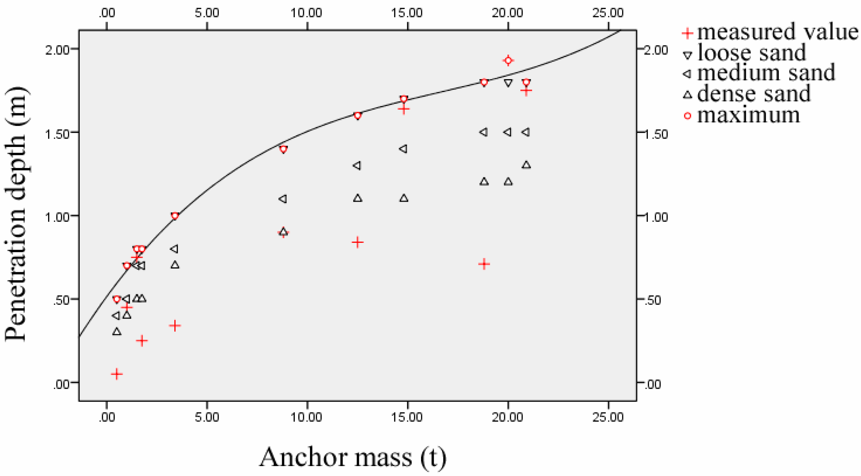
Figure 10 and
Figure 11 show the scatterplots of the measured and calculated values for the penetration depth in clay and sand, respectively. The red circle represents the maximum measured and calculated values for the same penetration depth.
By comparing the calculated value with the measured value, it was found that the measured value under the clay condition was mostly distributed within the range of the maximum value and the minimum value, indicating that the calculated value and the measured value under the clay condition have a good consistency. However, under the condition of sandy soil, some measured values were lower than the minimum value of calculated values, which may result from the composition of sandy soil being more complex, and the fitting in this paper was the maximum value of measured values and predicted values, so this result has good safety in the protection of submarine pipelines.
Based on the fitting goodness of each model, the model test results, and other related indicators, the most suitable curve model was used to perform the nonlinear regression of various curve models on the anchor’s mass and the corresponding maximum penetration depth. The fitting indicates that the anchoring penetration curves of the two substrates can adapt to the regression fitting model of the cubic curve. Equations 29 and 30 are the regression equations for anchor penetration in clay and sand, respectively, which are fitted using a numerical method.
A ship’s anchor penetration under sufficient water depth can be effectively estimated using the aforementioned regression equation, which provides a basis for analyzing anchorage accidents in submarine pipelines and a reference for safe buried pipeline depths in submarine pipeline engineering.
5. Conclusions
In this study, the movement process of an anchor in water and when it penetrates seabed soil was analyzed based on relevant data, literature, and theories. A calculation method and program for penetration were then developed. The calculation results of penetration depth were verified based on the measured penetration data, which proved the credibility of the proposed calculation method for penetration depth. Furthermore, a regression equation for estimating the penetration depth of an anchor in actual, complex cases was proposed.
The main research results and conclusions of this study are summarized as follows:
(1) A calculation method for anchor bottoming speed was developed, and its relationships with anchor mass, horizontal projected area, the aerial altitude of the anchor above the water surface, and water depth were analyzed.
(a) The bottoming speed increased with an increase in anchor mass.
(b) The bottoming speed increased with a decrease in the projected area of the anchor’s horizontal plane.
(c) The bottoming speed increased with an increase in the aerial altitude of the anchor. However, the bottoming speed was independent of altitude when the water was sufficiently deep.
(d) The bottoming speed of the anchor increased with an increase in water depth when the aerial altitude of the anchor was low. The bottoming speed of the anchor increased with an increase in water depth when altitude was high. The bottoming speed did not change with an increase in water depth when the water was sufficiently deep.
(2) A calculation method for anchor penetration depth was obtained by further utilizing the anchor’s bottoming speed.
(3) A calculation program for penetration depth was designed using MATLAB. Combined with anchoring experimental data, the calculated penetration depth was verified to prove that the simulation method for penetration depth and the results obtained in this study exhibited good credibility.
(4) The approximate relationship between anchor mass and maximum penetration in clay and sand was obtained after data analysis and processing, considering the diversity and complexity of seabed soil composition in actual conditions. The result was safe to be used to estimate the penetration of an anchor with a certain mass in clay and sand. Thus, the findings of this study provide a reference for analyzing anchorage accidents in submarine pipelines and for determining the safe buried depth of submarine pipeline projects.
Under the condition of clay substrate, the predicted results of regression equation were in good agreement with the measured values. However, under the condition of sandy soil substrate, the prediction results of regression equation were obviously larger than the measured value, which is a limitation of this study, but is safe for the buried depth of submarine pipelines.
It is worth mentioning that with the development of Marine geological survey technology in the future, more and more attention will be paid to the accurate calculation of anchor penetration. Future studies should further analyze the accurate prediction of penetration under sandy soil substrate conditions to facilitate the application of anchor penetration to the buried depth of submarine pipelines.


