Article

Effect of Tidal Stage on Sediment Concentrations and Turbulence by Vessel Wake in a Coastal Plain Saltmarsh

U. S. Army Engineer Research and Development Center, Coastal and Hydraulics Laboratory, 3909 Halls Ferry Road, Vicksburg, MS 39180, USA
*
Author to whom correspondence should be addressed.
J. Mar. Sci. Eng. 2019, 7(6), 192; https://doi.org/10.3390/jmse7060192
Submission received: 9 May 2019 / Revised: 13 June 2019 / Accepted: 17 June 2019 / Published: 22 June 2019

Abstract

:
Vessel generated waves can impact shoreline stability and habitat structure in many waterways. Sheltered regions, such as coastal plain saltmarshes, support fragile ecosystems and can be particularly vulnerable to the effects of unregulated vessel operations. Instruments for measuring currents and sediment concentration were deployed in a coastal plain saltmarsh to examine the small-scale physical characteristics of the vessel wake generated by recreational craft typical of this environment. The response to vessel wake varied sharply depending upon the stage of the tide. At low tide, waves breaking on the exposed bank produced high concentrations of suspended material that were transported offshore through turbulent diffusion. When the water elevation exceeded the toe of the marsh scarp, the concentration and turbulent kinetic energy exhibited less of a statistically significant variation in response to vessel passage. For the most energetic flows, the vessel orbital velocities were dwarfed by turbulent fluctuations generated by the sheared tidal boundary layer. While further research is required, preliminary findings indicate that the dissipation of vessel wake energy may stimulate or enhance shear generated turbulence if the characteristic wave period is similar to the characteristic time scale of the energy containing eddies.

1. Introduction

Vessel generated waves in shallow water can impact shoreline stability and habitat structure in many waterways [1,2,3,4]. These impacts are linked to sediment transport processes, which are associated with dissipation and turbulence generation similar to wind waves, tides, or other energetic forcing mechanisms. Unlike wind waves or tides, vessel generated waves propagate as discrete packets, and the resulting energy dissipation, turbulence generation, and sediment transport are short lived. As such, the impact of vessel wake in estuaries with sufficient fetch is often dwarfed by the integrated effect and persistence of wind wave attacks [5]. However, seasonal patterns (e.g., non-storm summer conditions in which wind wave energy is reduced) and periods of elevated boating activity on weekends or during holidays can increase the relative contribution of vessel wake to energy dissipation at the shoreline in estuaries with a larger fetch [6,7,8]. Also, different regions of the same estuary can experience much weaker wave conditions due to fetch limitations in areas that are sheltered from the more exposed open bay, thereby allowing vessel wake to represent the dominant form of wave energy.
While a large body of literature exists on the shoreline erosion and sediment transport caused by vessel wake, fewer process-based studies have focused on saltmarshes in particular [5,9]. Previous studies have mainly concentrated on vessels operating near fringing saltmarshes, where the primary wake sources are commercial vessels including container ships, pilot boats, barges and tankers [10,11]. Container ships and tankers can generate large wakes, especially the drawdown, which can produce 0.5 to 1 m fluctuations in water level that dominate the water surface elevation signal and associated wave energy flux [11]. In addition to these long waves, the bow waves generated by larger vessels have the capacity to produce wake heights that are generally higher than wind waves but with a much shorter duration [12]. Wake height also decays away from the vessel sailing line so that the effect diminishes with distance from the channel [13]. However, the vessel wake from high speed ferries have been shown to impact the shoreline as far as 3 km from the source [2].
In contrast, recreational craft can penetrate the marsh interior, where vessel wake originating in the navigation channel may not reach, and fetch limitations reduce the potential for wind wave growth. Even though recreational craft typically do not generate waves as large as commercial vessels, due to their proximity, they directly affect more vulnerable regions of the wetland interior that otherwise do not experience any impact from vessels operating in navigation channels. Considering that recreational vessel use is on the rise globally [14], coastal plain saltmarshes can expect to see an increase in the number of small craft and a greater potential for accelerated erosion along the marsh edge.
The effect of waves on the bed is frequency and depth dependent, so that the shorelines in intertidal areas are subjected to vastly different wave stress conditions depending upon the stage of the tide. Tonelli, et al. [15] used a Boussinesq model to investigate wave forcing on marsh boundaries as a function of tidal stage. Their results showed marked differences in wave thrust and maximum bed shear stress as a function of tidal stage and marsh edge morphology. Maximum thrust occurred just below the top of the marsh platform when the wave impinged on a vertical scarp but then decreased rapidly as the water depth exceeded the marsh elevation. The associated sediment transport characteristics are presumably also linked to tidal stage, so suspended sediment concentrations are greater when the bank is exposed and reduced when the marsh is submerged. The tide-induced stress along the marsh boundary likewise varies as a function of water level. In the classic ‘pumping mode’, maximum flow speed occurs around mid-tide, but in a mixed tidal regime, the actual elevation compared to the marsh platform will be somewhat modulated. In natural systems, friction and bay morphology distort tidal wave propagation, and the elevation of maximum flow can vary widely depending upon the relative amplitude of the dominant over-tide constituents [16]. Not only should the vessel wake stress distribution as a function of tidal stage be considered, but also how it compares to the timing and magnitude of the maximum stress generated by the tidal flow.
While the mechanics of vessel wake have been studied in terms of wake structures generated by various vessel types and the general relationship between wake height and sediment concentration [9,17,18], the detailed sediment flux and turbulence characteristics due to small recreational craft as a function of tidal stage in the presence of energetic tidal forcing has not been investigated. The purpose of this paper is to present the results of a field study to examine the hydrodynamic and sediment transport characteristics of vessel wake in an intertidal saltmarsh as a function of tidal stage focusing on small-scale physical processes. Investigating the fine-scale processes reveals information necessary to advance the present understanding of the complex and transient nature of vessel impacts. This study can help to improve wake models and provide operational guidance to inform management strategies aimed at protecting vulnerable wetland ecosystems.
The following section describes the setting and field deployment. The results focus on the relationship between tidal stage and vessel-induced sediment resuspension and turbulence, as well as the acute stimulation and persistence of turbulence subsequent to vessel passage. The discussion highlights the importance of tidal stage, tidal currents, and wake energy on the overall shoreline dynamics of an intertidal coastal plain saltmarsh. The discussion presents evidence that vessel wake, though transient, may stimulate boundary generated turbulence through a yet unresolved transport mechanism associated with wave breaking.

2. Materials and Methods

The study was carried out in the North Inlet estuary located near Georgetown, South Carolina USA (Figure 1). The North Inlet is a coastal plain saltmarsh consisting of low-relief mud flats dissected by a sinuous network of sub-and intertidal channels. The system receives little freshwater input, and the hydrodynamics are dominated by tidal processes. The tidal range at the entrance is 1.5 m, with maximum current speeds in the inlet throat that vary between 0.5 and 1.0 m/s as a function of the fortnightly tide [19,20]. The North Inlet is fronted by a barrier island complex, so there is very little wind wave influence, except possibly during periods of high water associated with the coastal setup combined with spring tide conditions. However, the North Inlet experienced little impact from Hurricane Hugo, a Category 4 hurricane that made landfall approximately 60 km south of the study site, due in part to the storm surge (3–4 m), which submerged the marsh platform protecting the surface from direct wave attack [21].
The study was carried out over a 2 day period by deploying sensors to measure flow and sediment concentrations on the bank of two sub-tidal channels. The first day, the instruments were deployed on an oyster bank in Old Man Creek (Station 1). The second day, the instruments were redeployed along an oyster-free section of Town Creek further from the inlet entrance (Station 2). The channel width was 250 m and 60 m at Station 1 and Station 2, respectively. The instrument package included a pair of Sontek acoustic Doppler velocimeters (ADVs). Estimates of the bank slope were determined from the ADV tilt sensor to be 0.11 at Station 1 and 0.26 at Station 2. The slope was relatively uniform from the instruments to the toe of the scarp, which was approximately 0.85 m and 1.30 m above the bed, as measured from a point directly beneath the ADV sampling volume at Station 1 and Station 2, respectively (Figure 2). The top of the marsh scarp, which coincided with the elevation of the marsh surface, was approximately 1.10 m (Station 1) and 1.80 m (Station 2) above the height of the location of the ADVs. The elevation of the instrument package was not referenced to a common tidal datum, so the reported water levels are measured relative to the local bed.

2.1. Current and Shear Stress Measurements

The ADVs were deployed on a single frame and vertically stacked, with the lower sensor (denoted N246) positioned 0.22 m above the bed and the upper sensor (denoted N230) positioned 0.40 m above the bed (Figure 2). The current probes were mounted at the end of a pair of lateral arms that extended from a rectangular frame containing the electronics (Figure 3). The lateral arms were oriented normal to the channel axis to prevent obstruction of the wake flow as it propagated past the instrument package. The orientation also made it possible to record the along channel tidal current without obstruction. The velocity vector (u, v, w) was divided into burst averaged (U, V, W) and fluctuating (u′, v′, w′) components. The coordinate system was chosen such that u was cross-channel (+toward the bank), v was along channel (+during flood), and w was vertical (+upward). The ADVs were programmed with a sampling frequency of 10 Hz for a 15 min burst every 20 min. Wave height was not measured directly, but the instrument package was equipped with a pressure sensor to measure the burst-averaged water level.
The burst-averaged Reynolds stress (τc) is written in terms of the kinematic shear stress τ c = ρ u 2 , where ρ is the fluid density. The kinematic shear stress, which is the square of the shear velocity (u*), is computed using the direct covariance method of the fluctuating velocity components,
u 2 = u w v w
where the brackets denote a temporal average over a burst. The turbulence kinetic energy (TKE) is calculated as
  T K E = 1 2 [ u 2 + v 2 + w 2 ] .
The bottom stress associated with the vessel wake (τw) is written as
    τ w = 1 / 2 ρ f w U b 2  
where fw is the wave friction factor and Ub is the orbital velocity. The amplitude and period of a wake group varies between individual waves, which also modulates the shear stress attributed to the vessel wake. In practice, the maximum bottom shear stress over a wave cycle is used in sediment trasport models. As such, the maximum bottom orbital velocity for each vessel wake group is used to compute τw. This leads to a conservatively high estimate for the shear stress generated by vessel wake and provides a reasonable upper bound on the sediment transport potential. The friction factor and associated wave stress are computed using the bottom boundary layer model of Styles and Glenn for pure waves [22]. The friction factor is a function of the relative roughness defined as z0/Ab, where z0 is the hydraulic roughness and Ab is the bottom excursion amplitude, (=Ub/ω) and ω is the radian frequency [22,23]. The orbital velocity is computed from the time series measurements by extrapolating the velocity at the sensor to the bed using linear wave theory. The radian frequency is determined as the peak period Tp (=2π/ω) from measurements of the zero-crossing of the largest amplitude wave in the time series. The bottom roughness is set to a constant of 3.0 × 10⁻⁴ m, which is reasonable for tidal creeks in the North Inlet [24].

2.2. Time–Frequency Analysis

The time–frequency domain analysis of the velocity and concentration is conducted using a wavelet transform [25]. A wavelet analysis is akin to time series spectral analysis such as the well-established Fourier transform method [26]. Unlike spectral analysis, which applies the basis functions to the full time record, the time domain is divided into discrete overlapping segments. The spectral analysis is applied independently to each segment, and the resulting segments are reconstructed to give the original signal amplitude and phase as a function of frequency (period) and time.
Wavelet analysis has a strong appeal for elucidating the spectral signature of time series containing turbulence fluctuations that are intermittently interrupted by vessel passage, and wavelet or spectrogram techniques are increasingly being applied to investigate time series measurements of vessel wake [27,28,29,30]. Vessels produce a narrow banded signal with finite temporal duration in an otherwise wider band signal. Thus, the frequency dependent time window of a wavelet is ideal for extracting the spectral characteristics of vessel wake even in the presence of wind waves and turbulence, assuming that the vessel wake is sufficiently separated in frequency or amplitude space from the other sources of flow energy. Once the vessel wake signature is identified, the spectrum can be integrated to give the wave height variance and the location of the spectral peak.
Wavelet analysis is performed using the “Cross wavelet and wavelet coherence toolbox for MATLAB” [31]. The package produces the energy density as a function of time and period. The analysis is applied to each burst and used to isolate the wave period and wave energy of individual wakes. It is also applied to the concentration time series to reveal fluctuations in the spectral signal caused by either vessel wake or turbulence.

2.3. Vessel Wake Measurements

Vessel wake was generated with a 21 ft Boston Whaler Outrage equipped with a single 150 kW outboard engine, which is typical of powered recreational craft operating in coastal and estuarine environments. The vessel was constructed with the following characteristics: beam = 2.2 m, length = 6.5 m, draft = 0.23 m, and dry mass = 1110 kg. In all experiments, the boat sailing line was parallel to the channel axis and all but one of the vessel passes occurred within 30 m of the shoreline. The final pass on the first day at Station 1 occurred near high tide at 125 m from the bank. The number of vessel passes during a single burst varied between one and five in order to measure the cumulative effect of multiple passes within a short timeframe and to generate a range of wake heights. The passes occurred at different tidal stages and different ambient flow velocities in order to investigate the hydrodynamics and sediment dynamics associated with the vessel wake in an inter-tidal saltmarsh with energetic tidal currents. A total of 38 vessel passes were conducted over the two day study in 13 separate bursts. Vessel passes 30 through 37 occurred during maximum flood when the along-channel current exceeded 0.35 m/s. Because of the increased turbulence due to the higher flow, it was not possible to visually identify the vessel-induced orbital velocities in the time record, and, thus, these vessel wake events were not included in the analysis.

2.4. Sediment Concentration

Sediment samples were acquired with one liter bottles by placing them adjacent to the ADV sampling volumes and then removing the caps and allowing them to fill underwater. Eighteen samples were collected adjacent to each probe. The lower ADV (N246) was sampled first, and then the upper ADV (N230) was sampled approximately 30 s later. The time to fill the bottle was approximately 10 s. The time (to a 1 s accuracy) that the cap was removed was recorded and later correlated with the ADV clock for regression analysis. To capture a range of concentrations, samples were acquired at different tidal stages.
The samples were returned to the laboratory for total suspended sediment (TSS) analysis. Each sample was filtered through a 1.5 µm glass filter. The filter was wet weighed and then dried at 100 C in a gravity-convection oven for 24 h. TSS was calculated as the difference between the dry filter weight before and after the analysis.
Acoustic backscatter measurements were converted to TSS using the regression equation
  log 10 ( c m ) = m A B S + b
where cm is the measured concentration, ABS is the acoustic backscatter signal from the ADV, and m and b are calibration constants. The samples were regressed against the acoustic backscatter data to determine the fitting parameters [m, b]. The concentration and acoustic backscatter were positively correlated for both instruments, with N246 producing a higher regression coefficient (r2 = 0.70) compared to N230 (r2 = 0.33). The corresponding p-values were 0.001 and 0.18 for N246 and N230, respectively. The lower correlation coefficient combined with the higher p-value for N230 indicated less confidence in the regression analysis for this instrument. Therefore, the regression equation was applied only to N246 to produce a modeled time series of the suspended sediment concentration that was synchronized with the velocity measurements. The modeled concentration, c, was likewise divided into burst averaged, C, and turbulent fluctuations, c′.

3. Results

The tidal hydrodynamics are used to place the vessel wake measurements in the context of the ambient forcing and to depict the tidal stage associated with vessel passage events. The burst averaged water depth indicates a mixed tidal regime with a high-high tide followed by a low-high tide (Figure 4). The gap in the record denotes the recovery of the instruments at Station 1 and redeployment at Station 2. The majority of bursts with vessels occur on the rising limb of the tide during the high-high phase. Morphologically, the vessel passes occur near low tide when the bank is exposed, at mid-tide when the scarp is exposed and tidal currents are strongest, and near high tide when the scarp is submerged and the wake propagates over the marsh surface. The extremes in the along-channel current occur during the rising or falling limb of the tide (hours 4, 16, 29, and 43). Peak flows are higher at 0.40 m above the bed, indicating a vertically sheared flow field and greater turbulence production typical of a shallow tidal boundary layer. The highest flows occur near mid-tide when the water level coincides with the toe of the scarp. While the range of water depths for bursts with vessel passages are similar, the maximum tidal currents are higher at Station 2. The minimum suspended sediment concentration occurs near slack tide and generally increases with flow speed. There is some variability around this trend, especially during the first day when maximum current speeds are lower, and concentrations are higher, just prior to the slack tide. These times correspond to vessel wake passages, when the water column sediment flux is due to vessel wake in addition to the currents.

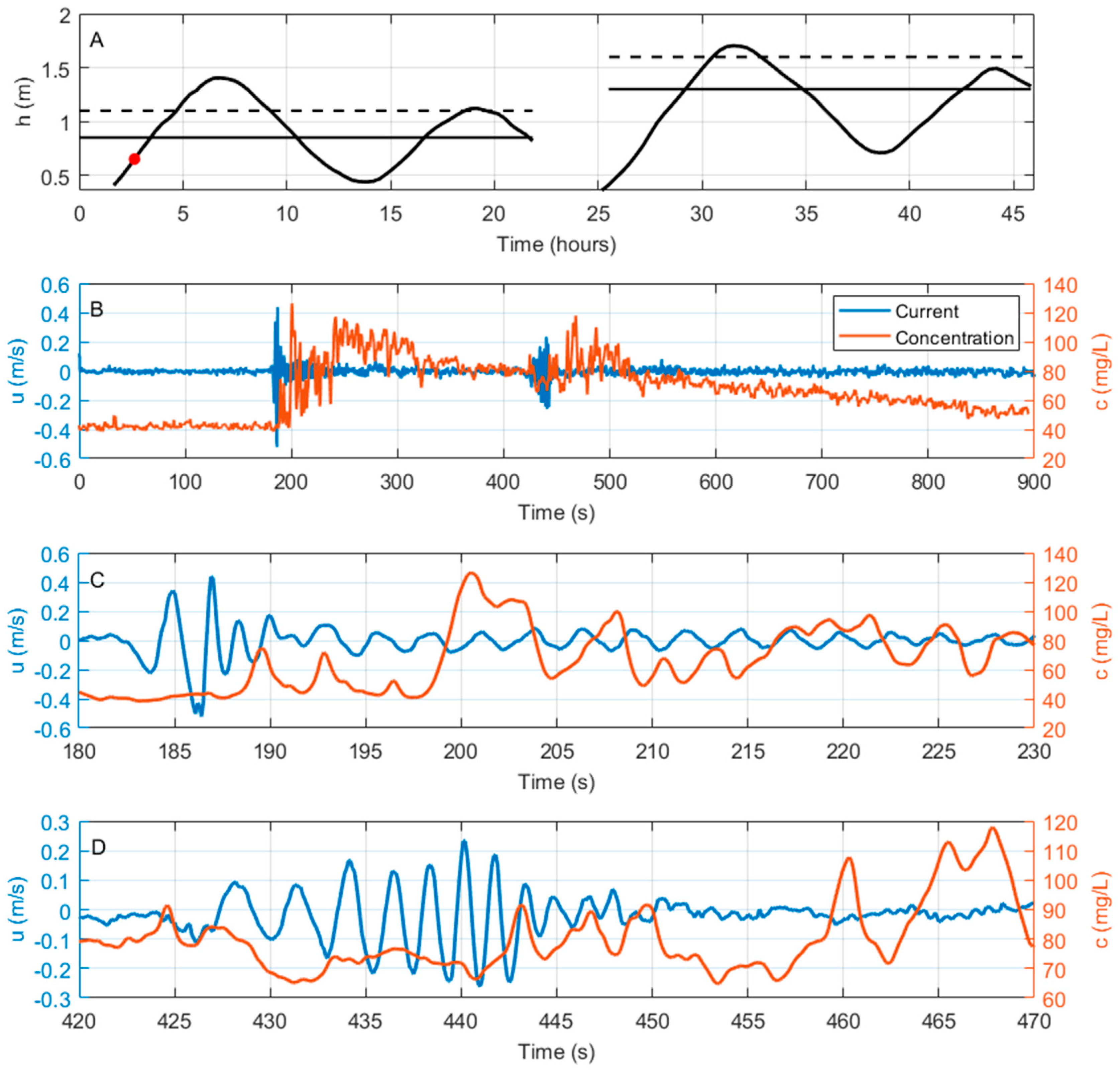
3.1. Vessel Wake Hydrodynamics and Sediment Resuspension

An example illustrating two vessel wake events is depicted in Figure 5. The figure depicts the first burst with vessel wake at Station 1 (hour 3, Figure 4) and occurs on the rising limb of the tide shortly after the sensors are submerged. Vessel-induced wake is identified in the cross-shore current time series at approximately three (180 s) and seven minutes (420 s), respectively, into the record. The vessel speed and trim during the first passage are chosen to produce a large wake to maximize sediment resuspension. During the second vessel passage, the speed is increased so that the vessel is planing. The wave form for both vessel passages is typical of a divergent wave, in which the amplitude envelope increases during the first few waves, reaches a peak near the midpoint, and then decays. The wave period becomes shorter with each passing wave, indicative of a dispersive wave pattern. The peak period for each vessel passage is 2.0 s and 1.7 s, respectively. The wave direction, as determined by the angle of maximum variance of the cross-shore and alongshore velocity components, indicates that the wake crest with respect to the shoreline approached at an angle of 28 degrees during the first pass and −20 degrees during the second pass. The sign change is because the vessel was traveling in the opposite direction during the second pass.
The suspended sediment concentration prior to the first wake event averaged 41 mg/L. As the wake propagated past the sensor, the concentration spiked to about 70 mg/L at approximately 3 and 6 s after the peak orbital velocity. The concentration returned to background levels for about 4 s. It then increased in a series of large amplitude fluctuations until about 221 s, after which it began an overall decrease until the second wake event. The concentration remained fairly steady as the first few waves from the second vessel passage propagated over the sensor but then showed small amplitude fluctuations at the trailing edge of the wave group and after the waves had passed. The largest increase apparently related to the vessel wake (460 s) occurred 20 s after the peak orbital velocity (440 s). It then increased in a manner similar to the first wake event until about 480 s, but the highest concentrations did not exceed the maximum concentrations following the first vessel passage. The concentration then decreased for the remainder of the burst. The increase in concentration after each burst was accompanied by large amplitude fluctuations that did not correspond to the period of the vessel wake.
The time delay between maximum concentration and orbital velocity indicates that sediment dynamics are not entirely driven by local resuspension due to wave-induced bottom stresses generated directly beneath the sensor. Rather, the delay is due to wave breaking on the shoreline, backing the instruments followed by the cross-shore transport of turbid water from the bank to the measurement point. This occurred after the vessel wake propagated past the sensor, so there is not a direct transport mechanism that can be attributed to the instantaneous bottom stress associated with the oscillatory wake velocity.
The steady decrease in concentration following each wake event indicates that particles were settling and that the concentration was returning to pre-wake conditions. Extrapolating the rate of decrease from the point of highest concentration to the intersection with the background concentration is a measure of the time required for the particles to settle and for how long the excess material can be dispersed in the tidal channel. In this case the concentration returned to background levels by the end of the burst. Fitting a trend line to the time series indicates that it takes 7.5 min for concentrations to return to pre-wake conditions after the second vessel wake event.
The concentration and velocity time series for the other vessel passages with visible wake signals show similar trends, as depicted in Figure 5. The primary difference is that the response is muted as the depth over the sensors increases. The orbital velocity amplitude decreased, and the difference in concentration prior to and following vessel passage was not as great. Further, the cumulative effect of multiple vessel passages was to maintain higher concentrations in the water column until the last vessel pass was complete. The time lag between velocity and peak concentration depicted in Figure 5 was persistent for all vessel passages. Time series plots of concentration and velocity for each case can be found in Styles and Hartman [32].
It is noted that of the 38 vessel passages, 3 bursts (9 total passes) at Station 2, corresponding to depths of 0.90, 0.99, and 1.07 m (between hours 27 and 29 Figure 4), did not produce a visible orbital velocity signal, so it was not possible to conduct a vessel wake analysis. However, 3 bursts at Station 1 (between hours 4 and 6 in Figure 4) with similar water depths (0.94, 1.07, and 1.13 m) did produce visible orbital velocities. The along-channel current for the 3 bursts at Station 2 was 0.37, 0.39, and 0.48 m/s, and at Station 1, the current was 0.18, 0.02, and −0.09 m/s. The higher flow speeds at Station 2 produced large turbulent fluctuations that dwarfed the vessel wake signal, making it difficult to visually detect the orbital velocities with any degree of certainty.

3.2. Tidal Stage

Examining the velocity and concentration signals before and after vessel passage, and at different tidal stages, helps to elucidate the mechanisms responsible for the observed time lag and to quantify the attenuation of the wake signal as a function of water level. In order to compare and contrast the conditions just prior to, and immediately after, vessel passage, each 15 min burst is sub-divided into 20 s segments with a 5 s overlap. A fixed number of segments prior to vessel passage are averaged to compute pre-wake conditions. The same number of segments is averaged after vessel passage to ensure that the pre- and post-data are equally weighted for the statistical analysis. The post vessel passage timeframe begins after the last wake to ensure that the orbital velocities are not counted as turbulence. Ninety-five percent confidence limits are computed to quantify the statistical uncertainty. The time lag between maximum velocity and concentration makes it difficult to distinguish individual wake events for bursts with multiple vessel passes. As such, the post-vessel wake period is defined after the final pass.
When the water level is below the scarp, sediment concentrations are significantly higher subsequent to vessel passage (Figure 6). Once the water level exceeds the toe of the scarp but is still below the elevation of the marsh platform, concentrations begin to show less of a trend that would indicate a significant difference between pre- and post-vessel passage. At higher water levels, the wake impinges upon the steep scarp face at an elevation just below the marsh surface and at a greater distance from the location of the instruments. The variability, as measured by the error bars, indicates more energetic fluctuations about the mean subsequent to vessel passage when the bank is exposed. This difference diminishes as the water depth exceeds the toe of the berm and the marsh platform. The TKE is, likewise, higher after vessel passage when water levels are below the elevation of the scarp, but one instance is not statistically significant, as indicated by the overlap in the 95% confidence limits. The TKE also decays once the bank is submerged, which is an indication of the decrease in turbulence intensity as the water level approaches slack high tide and the mean current is reduced. The variability subsequent to vessel passage when the bank is exposed indicates the presence of energetic fluctuations presumable caused by vessel wake breaking at the shoreline and enhancement of the turbulence at the sensor location. The post-vessel passage variability decreases once the water level exceeds the bank but is below the top of the scarp. There is no significant difference between pre-and post- vessel passage once the marsh platform is submerged.
The results suggest that wave breaking, as opposed to local resuspension, is responsible for the observed time lag between wake passage and the increase in concentration. Sediment resuspended between the sensor location and the shoreline must be transported offshore to the ADV sampling volume, presumably through a combination of advection and cross-shore turbulent diffusion. Turbulent diffusion is measured by the cross-shore sediment flux, <cu′>. The sign convention for the current is chosen such that a positive sediment flux occurs when either a positive fluctuation in cross-shore velocity (onshore) is correlated with a positive fluctuation in concentration (instantaneous increase in concentration), or a negative fluctuation in the cross-shore velocity (offshore) is correlated with a negative fluctuation in concentration (instantaneous decrease in concentration). In either case, the average flux due to turbulent diffusion is directed shoreward, indicating the onshore transport of sediment. By the same analogy, a negative sediment flux indicates offshore sediment transport.
The cross-shore sediment flux prior to vessel passage is relatively small and does not vary greatly as a function of tidal stage, indicating little net sediment transport through turbulent diffusion (Figure 6). When the water depth is below the scarp, the cross-shore sediment flux subsequent to vessel passage is negative, indicating offshore transport. Once the water level exceeds the tow of the scarp, the magnitude decreases and the pre- and post-vessel passage results are not as disparate. The variability subsequent to vessel passage when the water depth is below the scarp indicates large turbulent fluctuations, which is consistent with the TKE results. Through turbulent diffusion, higher concentrations of resuspended material are transported offshore subsequent to vessel passage, and the magnitude of the transport diminishes as the water depth increases.

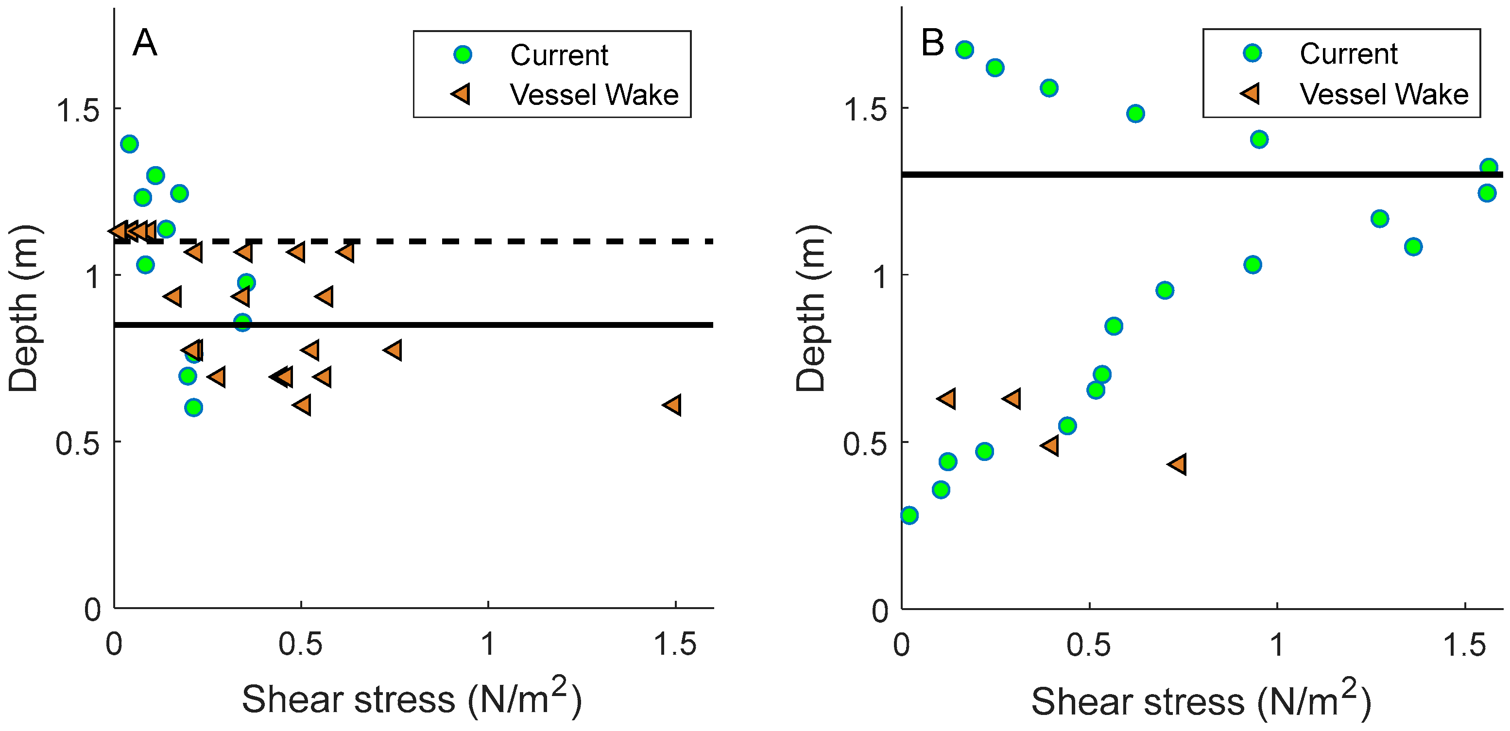
3.3. Bottom Stress in the Intertidal Region
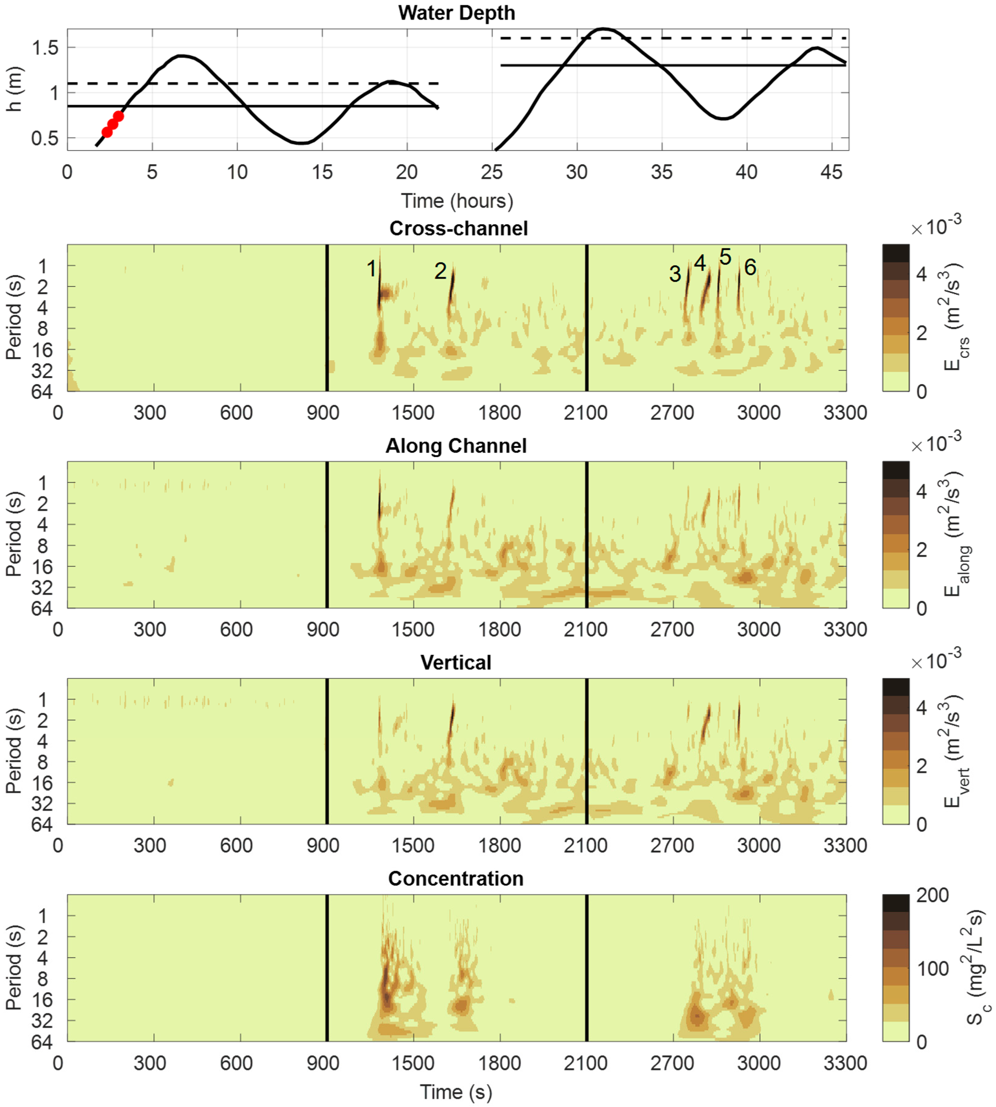
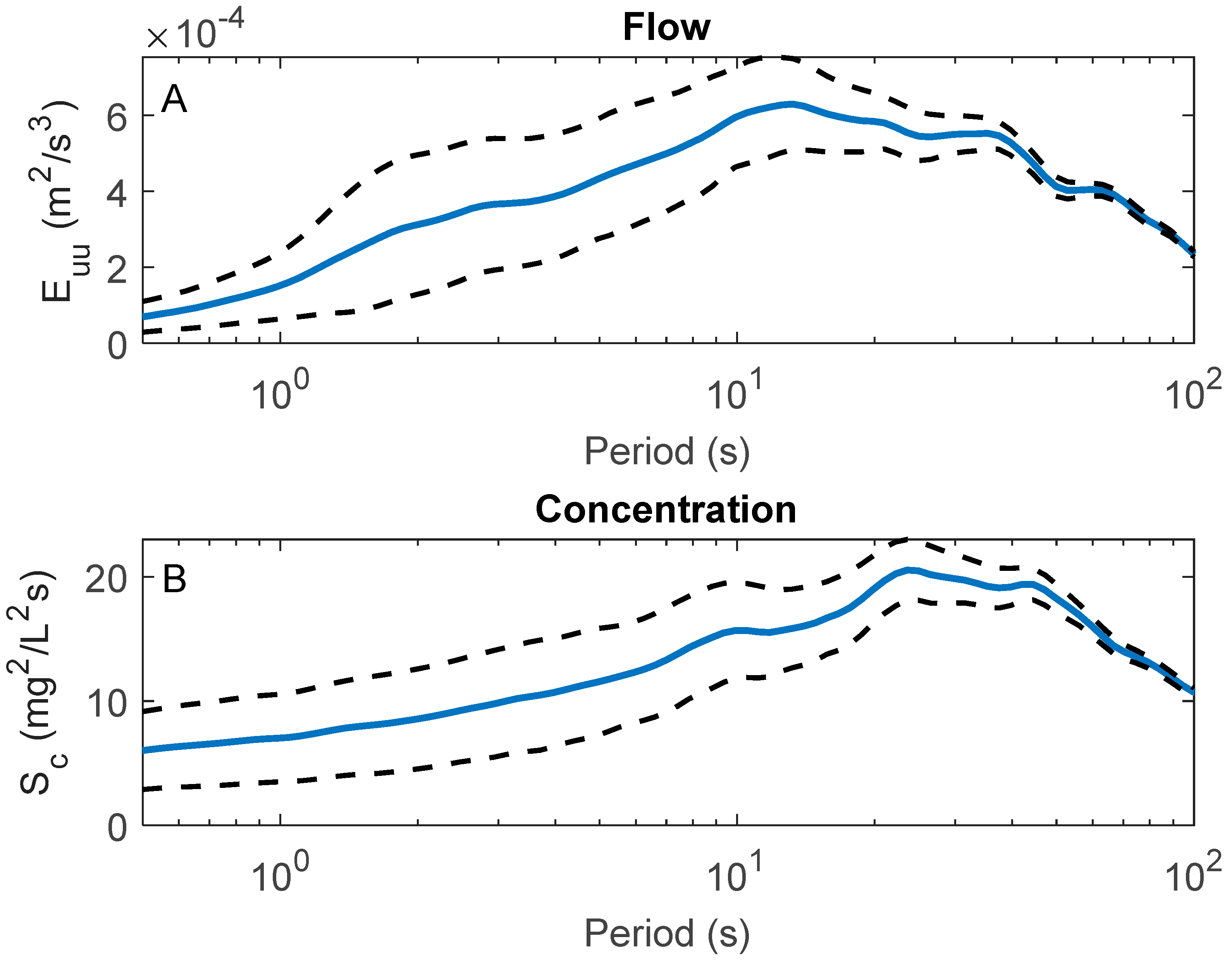
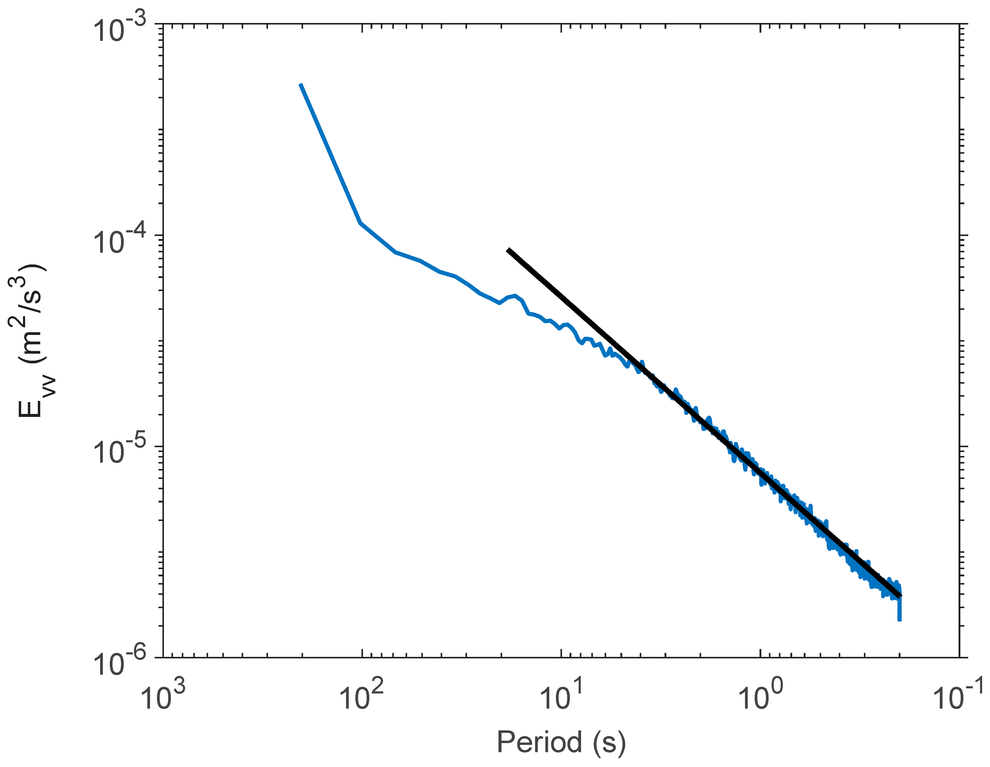
A measure of the relative contribution to energy dissipation at the bed between vessel wake and tidal currents can be expressed in terms of the shear stress as a function of water depth (Figure 7). Near low tide, the maximum shear stress associated with the vessel wake is greater than the shear stress generated by the tidal flow. The largest wave orbital velocities occur near low tide, when the water depth at the sensor location is a minimum. At the same time, the shear generated bottom stress due to the tidal current is weak as the flow switches from ebb to flood. As water depth increases, attenuation of the orbital velocities with depth decreases the bottom shear stress of the vessel wake, while the current shear stress increases until maximum flood. The field study includes multiple vessel passages at different speeds to produce a range of wake heights that could be generated during typical boating operations. Between low and mid-tide the magnitude of the vessel generated shear stress varies widely and, thus, is a function of vessel operations. This range of water depths coincide with the region of maximum tidal currents, and at Station 1 the vessel wake stress can easily exceed the current stress until the marsh platform is submerged. The four vessel passages that occur when the marsh platform is submerged (1.10 m), do not exceed the stress generated by the current. The maximum stress due to the tidal current never exceeds 0.4 N/m2, and the vessel wake is easily detectable at all water depths. At Station 2, vessel wake is detectable only for depths less than 0.70 m, despite the occurrence of vessel passes at depths of 0.90, 0.99, and 1.07 m. The stress associated with the current during maximum flood exceeds the vessel wake stress at any depth, even near low tide when the orbital velocities are largest.

3.4. Energy Spectra

Wavelet analysis is applied to examine the spectral characteristics of the kinetic energy and concentration. In order to place the effects of vessel passage in the context of the ambient conditions, the analysis focuses on the eighth, ninth, and tenth bursts. The eighth burst does not include a vessel passage, the ninth burst includes two vessel passages, which are illustrated in Figure 5, and the tenth burst includes four vessel passages. The bursts occur near low tide, so that the vessel wake impinges upon the bank at a point below the base of the scarp, producing high concentrations of suspended sediment. The wavelet diagrams show six very narrowly defined peaks in the energy density between 1 and 4 s, corresponding to the period of the vessel wake (Figure 8). The peaks are most visible in the cross-shore component (Ecrs) and less so in the along shore (Ealong) and vertical (Evert) components. The subtle shift from longer to shorter periods, as best illustrated in vessel passes numbered 2, 3, and 4, is indicative of dispersive water waves in which the longer waves arrive first. While occupying a narrow band in the time domain, the six peaks possess the highest energy density, indicating that the amplitude of the orbital velocities are greater than the turbulent fluctuations.
The wavelet diagrams also reveal a region of lower energy fluctuations in the ~8 to 32 s band that grows in intensity in conjunction with the initial vessel passage. The fluctuations reappear sporadically for the remainder of the record and are more pronounced in the along channel and vertical energy diagrams. The wavelet analysis identifies variability in the concentration (Sc) that includes intermittent fluctuations in the same range as the vessel wake but is more broadly banded. The region with the highest intensity is in the 8 to 32 s band, which is longer than the period of the orbital velocities but within the same range as the turbulence fluctuations in the velocity signal. Averaging the energy density for each of the other bursts with vessel wake as a function of the period reveals localized maxima in the concentration and energy spectra that are uncorrelated with the orbital velocities (Figure 9). It is noted that the fluctuations become more energetic, as the along channel velocity increases even when vessels are not present. In other words, the fluctuations in the 8 to 32 s band become more energetic as the tidal flow increases, indicating that the increase in intensity is an artifact of shear generated turbulence in the tidal boundary layer.

4. Discussion

It was shown that the offshore advection of material resuspended shoreward of the sensors reached the sensor location, which varied between 3 m and 8 m from the breaker point, depending upon the stage of the tide. Lingering particulate matter in the water column may disperse into the sub-tidal regions through offshore advection even if the majority of the wake energy dissipation and sediment resuspension occurs at the shoreline during breaking. This net offshore transport reduces the amount of sediment at the shoreline and redistributes it to deeper areas of the channel. Cross-shore transport in the aftermath of vessel passage has been implicated as a cause for bank erosion in coastal wetlands similar to the North Inlet [33].
The vertical variability in the pre- and post-vessel passage depends upon both the wake energy at breaking and the distance to the breaker point. If the source of sediment resuspension is further from the platform at high tide, and the cross-channel flux is primarily driven by gradient diffusion, then the magnitude of the concentration and sediment flux measured at the sensor location will be reduced. This explains the convergence between pre- and post-vessel passage results as water depth increases.

4.1. Shear Stress, Water Depth, and Bed Erosion Potential in the Intertidal Regime

The stress-stage diagram is a useful means to illustrate the vessel wake and tidal influence on sediment dynamics and bed stability in the saltmarsh intertidal regime. If the maximum stress due to the vessel wake does not exceed the maximum stress due to the tidal current, then the tidal current exerts the greatest force on the bed over a tidal period. In terms of the maximum force as a function of tidal stage, the tidal current will dominate at all elevations for which the tidal stress exceeds the wake stress. This excludes the fraction of the tidal phase near slack low or high tide, when it is more likely for the vessel wake stress to exceed the current stress. However, the region below mid-tide will experience greater stress due to the current during maximum flows. This implies that any reworking of bed sediment at low tide due to vessel wake could be dwarfed by the current during the subsequent maximum flood. Therefore, vessel wake effects will be greatest around high tide when currents switch from flood to ebb.
Other factors, such as the number of vessel waves per unit time (which is a function of vessel traffic density) and energy over threshold for sediment motion, also play a role in predicting the cumulative erosion potential of vessels. Maynord, Biedenham, Fischenich and Zufelt [8] showed that increased recreational vessel activity in the Kenai River, Alaska on holiday weekends led to vessel wake energy dissipation estimates that were 16% of the energy dissipated by the average river flow. They argued that while the majority of erosive potential was due to river discharge, the intermittent effect of recreational craft could not be ignored. Another critical factor is the wave stress at breaking, which was not measured but would indicate the total erosive potential at the waterline. However, if the stress at the waterline due to waves is universally less than the maximum stress due to the current, then the currents are still likely to dominate, at least for points below the elevation of maximum current stress.

4.2. Energy Spectra

The wavelet diagrams show randomized small-amplitude fluctuations in the 8 to 32 s band that appear shortly after vessel passage and then persist for the remainder of the burst. The concentration shows a similar pattern within the same band. However, the concentration fluctuations decay after vessel passage. This is due to particle settling, which reduces concentrations and the amplitude of the associated fluctuations. The timing and appearance of fluctuations in both the velocity and the suspended sediment concentration suggest that breaking may act to enhance turbulence motion in a lower frequency band. Because the increase in concentration is due to the energy dissipated at the shoreline at breaking rather than local resuspension, fluctuations in the concentration do not necessarily correlate with the vessel wake period. However, if turbulence intensity increases subsequent to breaking, as is shown here, then it is more likely that any observed fluctuations in the concentration correspond with the turbulence. Model studies have predicted the offshore turbulence convection of suspended sediment under breaking waves in the swash zone, supporting the idea of cross-shore turbulence convection [34]. Thus, concepts applied to breaking wind waves regarding the frequency of the uprush and retreat, as well as the turbulence convection process, may help to increase the present understanding of vessel wake dynamics.
While the appearance of fluctuations in the energy density and concentration after vessel passage suggests some degree of response to the vessel wake, the results are insufficient to draw a direct causal link in terms of the dynamical forcing mechanisms. For example, what is the likely source of the intermittent peaks in the energy density in the 8 to 32 s band revealed in the wavelet diagrams? They do not appear to be linked to the orbital velocities, which have much shorter periods (1.5–3 s). If the peaks are a product of boundary layer turbulence as opposed to vessel wake, then it is likely that they reside in the spectral range of the most energetic and persistent turbulent eddies [35]. Persistence in the absence of vessel wake suggests that the source is the boundary shear generated by the larger scale tidal current. Examination of the along channel component of the energy spectrum reveals a “–5/3” slope for periods shorter than about 6 s (Figure 10). This region of the energy spectrum corresponds to the inertial-subrange, in which larger eddies transfer energy to smaller eddies through a dissipative energy cascade [35]. The break from the “–5/3” slope at periods longer than about 6 s marks the transition between the inertial sub-range and the larger energy containing eddies. These eddies are presumably generated by the vertically sheared tidal flow, as the energy density in this band is greater for the along-channel and vertical components. This suggests that the turbulence fluctuations seen in the wavelet diagram are generated by the tidal flow and not directly tied to the vessel wake. Therefore, the presence of fluctuations in the energy density and concentration in the 8 to 32 band after vessel passage is consistent with the boundary layer theory.

5. Conclusions

The primary mechanism for sediment resuspension is wave breaking on the bank. This was based on the observed time lag between vessel passage and the increase in concentration that could not be explained under the assumption of local resuspension. When the bank was exposed, concentrations increased by a factor of two or more and remained elevated for several minutes after vessel passage. At higher flow speeds, the orbital velocity signal was undetectable at Station 2, even though the bank was exposed and the water depths were similar to bursts at Station 1 with easily identifiable vessel wakes. The energetic along-channel current produced turbulence fluctuations that dwarfed the smooth oscillatory signal associated with the waveform. Similarly, the concentration did not possess the characteristic increase and slow decay after vessel passage, so it was not possible to distinguish between tidally induced and vessel wake resuspension.
The vessel characteristics (vessel type, dimensions, and outboard motor) are typical of powered recreational craft operating in coastal and estuarine environments. While speed was not measured, the test conditions were chosen to generate a range of wake heights to represent what would typically be expected in similar intertidal environments. Local resuspension, even under the most energetic conditions, was small or absent compared to wave breaking on the shoreline. In areas where the saltmarsh is protected from wind waves, the breaking vessel wake can be a major, although intermittent, contributor to sediment transport at the shoreline. While regulating vessel speed has been suggested as a measure to reduce wake impacts [36], altering transit times to coincide with high tide may reduce total suspended sediment concentrations and the potential for vessel-induced bank erosion in intertidal areas. However, this would shift the location of greatest energy dissipation to the marsh interior, where flow resistance due to vegetation attenuates the freely propagating wake [37]. This process is still an active area of research, so the implications of vessel transits at high tide to shore protection are unclear.
Stress-stage diagrams provide a way to help gauge the impact of vessel wake in regions with energetic tidal currents. The maximum stress induced by vessel wake on the submerged bank may always be exceeded by the maximum tidal current stress, regardless of typical (e.g., small recreational craft) vessel operations. Landforms that are inundated below high tide may experience intermittent wake impacts that produce stresses and higher energy dissipation, but if the maximum stress due to the current exceeds the wake stress, then the long-term effect of vessels may be diminished even if instantaneous results suggest the opposite.
While some evidence has been presented to suggest that wake-induced breaking may stimulate turbulence, more analysis is required to unequivocally establish a direct dynamical relationship. If the breaking vessel wake can enhance turbulence in the band of the energy containing eddies, as suggested by the results, then a degree of phase coupling between the wake and turbulence would also be present. Measurements at the breaking point and direct estimates of runup and swash behavior would determine the characteristic timescales and amplitudes of the vessel generated wave field that could be compared to the timescales of the turbulence. Another issue that could be addressed with new measurements is related to the phasing of the vessel wake period and turbulence. What is the response of the mean flow if the characteristic period of the vessel wake is similar to the characteristic time scale of the energy containing eddies? An oscillatory flow imposed on a steady current has been shown to increase the energy density for periods shorter than the wave period [38], but these conclusions are based on a statistically steady wave field superimposed on a steady drift current. The effect of a transient vessel wake has not been explored, but it is possible that a similar coupling mechanism is present. If certain vessel operating conditions tend to generate wakes with periods comparable to the characteristic scales of the boundary layer turbulence, then there could be amplification of the energy dissipation due to resonance interactions between the independent signals. This could lead to greater sediment resuspension and possibly greater shoreline erosion than would occur if the two processes were assumed to function independently.

Author Contributions

Conceptualization and methodology were developed by R.S. Writing and draft preparation were conducted by R.S. and M.A.H. Visualization and editing were performed by M.A.H.

Funding

This research was jointly funded by the National Oceanic and Atmospheric Administration and by the Coastal Inlets Research Program and the Dredging Operations Environmental Research Program of the U. S. Army Corps of Engineers, Engineer Research and Development Center.

Acknowledgments

The authors would like to thank Steven Traynum for assistance in the field and the staff of the Belle W. Baruch Institute of Marine and Coastal Science for the use of facilities during the field data collection effort.

Conflicts of Interest

The authors declare no conflict of interest. The funders had no role in the design of the study; in the collection, analyses, or interpretation of data; in the writing of the manuscript; or in the decision to publish the results.

References

  1. Osborne, P.D.; Boak, E.H. Sediment suspension and morphological response under vessel-generated wave groups: Torpedo bay auckland, new zealand. J. Coast. Res. 1999, 15, 388–398. [Google Scholar]
  2. Kurennoy, D.; Soomere, T.; Parnell, K. Variability in the properties of wakes generated by high-speed ferries. J. Coast. Res. 2009, 1, 519–523. [Google Scholar]
  3. Herbert, D.; Astrom, E.; Bersoza, A.C.; Batzer, A.; McGovern, P.; Angelini, C.; Wasman, S.; Dix, N.; Sheremet, A. Mitigating erosional effects induced by boat wakes with living shorelines. Sustainability 2018, 10, 436. [Google Scholar] [CrossRef]
  4. Asplund, T. The Effects of Motorized Watercrafts on Aquatic Ecosystems; Bureau of Integrated Science Services and University of Wisconsin: Madison, WI, USA, 2000; Volume PUBL-SS-948-00. [Google Scholar]
  5. Houser, C. Relative importance of vessel-generated and wind waves to salt marsh erosion in a restricted fetch environment. J. Coast. Res. 2010, 26, 230–240. [Google Scholar] [CrossRef]
  6. Curtiss, G.M.; Osborne, P.D.; Horner-Devine, A.R. Seasonal patterns of coarse sediment transport on a mixed sand and gravel beach due to vessel wakes, wind waves, and tidal currents. Mar. Geol. 2009, 259, 73–85. [Google Scholar] [CrossRef]
  7. Laderoute, L.; Bauer, B. River Bank Erosion and Boat Wakes Along the Lower Shuswap River, British Columbia; Final Project Report Submitted to the Regional District of North Okanagan Fisheries and Oceans Canada; Larissa Laderoute & Bernard Bauer University of British Columbia Okanagan: Kelowna, BC, Canada, 2013. [Google Scholar]
  8. Maynord, S.T.; Biedenham, D.S.; Fischenich, C.J.; Zufelt, J.E. Boat-Wave-Induced Bank Erosion on the Kenai River, Alaska; U.S. Army Corp of Engineers: Vicksburg, MS, USA, 2008; p. 129.
  9. Cox, R.; Wadsworth, R.; Thomson, A. Long-term changes in salt marsh extent affected by channel deepening in a modified estuary. Continental Shelf Res. 2003, 23, 1833–1846. [Google Scholar] [CrossRef]
  10. Davis, S.E., III; Allison, J.B.; Driffill, M.J.; Zhang, S. Influence of vessel passages on tidal creek hydrodynamics at aransas national wildlife refuge (Texas, United States): Implications on materials exchange. J. Coast Res. 2009, 25, 359–365. [Google Scholar] [CrossRef]
  11. Maynord, S.T. Ship Forces on the Shoreline of the Savannah Harbor Project; U.S. Army Corps of Engineers: Washington, DC, USA, 2007.
  12. Kelpšaite, L.; Parnell, K.; Soomere, T. Energy pollution: The relative influence of wind-wave and vessel-wake energy in tallinn bay, the baltic sea. J. Coast. Res. 2009, 56, 812–816. [Google Scholar]
  13. Sorensen, R.M. Prediction of Vessel-Generated Waves with Reference to Vessels Common to the Upper Mississippi River System. In ENV Report 4; US Army Corps of Engineers: Rock Island, IL, USA, 1997. [Google Scholar]
  14. Burgin, S.; Hardiman, N. The direct physical, chemical and biotic impacts on australian coastal waters due to recreational boating. Biodivers. Conservat. 2011, 20, 683–701. [Google Scholar] [CrossRef]
  15. Tonelli, M.; Fagherazzi, S.; Petti, M. Modeling wave impact on salt marsh boundaries. J. Geophys. Res. Oceans 2010, 115, 1–17. [Google Scholar] [CrossRef]
  16. Blanton, J.O.; Lin, G.; Elston, S.A. Tidal current asymmetry in shallow estuaries and tidal creeks. Continental Shelf Res. 2002, 22, 1731–1743. [Google Scholar] [CrossRef]
  17. Anderson, F.E. Effect of wave-wash from personal watercraft on salt marsh channels. J. Coast. Res. 2002, 1, 33–49. [Google Scholar]
  18. Bauer, B.O.; Lorang, M.S.; Sherman, D.J. Estimating boat-wake-induced levee erosion using sediment suspension measurements. J. Waterw. Port Coast. Ocean Eng. 2002, 128, 152–162. [Google Scholar] [CrossRef]
  19. Wargo, C.A.; Styles, R. Along channel flow and sediment dynamics at north inlet, south carolina. Estuar. Coast. Shelf Sci. 2007, 71, 669–682. [Google Scholar] [CrossRef]
  20. Kjerfve, B. Circulation and salt flux in a well mixed estuary. In Physics of Shallow Estuaries and Bays; Van de Kreeke, J., Ed.; Springer: New York, NY, USA, 1986; pp. 22–29. [Google Scholar]
  21. Gardner, L.; Michener, W.; Williams, T.; Blood, E.; Kjerve, B.; Smock, L.; Lipscomb, D.; Gresham, C. Disturbance effects of hurricane hugo on a pristine coastal landscape: North inlet, south carolina, USA. Neth. J. Sea Res. 1992, 30, 249–263. [Google Scholar] [CrossRef]
  22. Styles, R.; Glenn, S.M. Modeling stratified wave and current bottom boundary layers on the continental shelf. J. Geophys. Res.-Oceans 2000, 105, 24119–24139. [Google Scholar] [CrossRef] [Green Version]
  23. Styles, R.; Glenn, S.M.; Brown, M.E. An Optimized Combined Wave and Current Bottom Boundary Layer Model for Arbitrary Bed Roughness; ERDC/CHL, TR-17-11; U.S. Army Corps of Engineers: Washington, DC, USA, 2017.
  24. Voulgaris, G.; Meyers, S.T. Temporal variability of hydrodynamics, sediment concentration and sediment settling velocity in a tidal creek. Continental Shelf Res. 2004, 24, 1659–1683. [Google Scholar] [CrossRef]
  25. Daubechies, I. The Wavelet Transform. Time-Frequency Localization and Signal Analysis. IEEE Trans. Inf. Theory 1990, 36, 961–1005. [Google Scholar] [CrossRef]
  26. Press, W.H.; Flannery, B.P.; Teukolsky, S.A.; Vetterling, W.T. Numerical Recipes; Cambridge University Press: Cambridge, UK, 1989; Volume 3. [Google Scholar]
  27. Houser, C. Sediment resuspension by vessel-generated waves along the savannah river, georgia. J. Waterw. Port Coast. Ocean Eng. 2011, 137, 246–257. [Google Scholar] [CrossRef]
  28. Didenkulova, I.; Rodin, A. A typical wave wake from high-speed vessels: Its group structure and run-up. Nonlinear Process. Geophy. 2013, 20, 179–188. [Google Scholar] [CrossRef]
  29. Torsvik, T.; Soomere, T.; Didenkulova, I.; Sheremet, A. Identification of ship wake structures by a time–frequency method. J. Fluid Mech. 2015, 765, 229–251. [Google Scholar] [CrossRef]
  30. Sheremet, A.; Gravois, U.; Tian, M. Boat-wake statistics at jensen beach, florida. J. Waterw. Port Coast. Ocean Eng. 2012, 139, 286–294. [Google Scholar] [CrossRef]
  31. Grinsted, A.; Moore, J.C.; Jevrejeva, S. Application of the cross wavelet transform and wavelet coherence to geophysical time series. Nonlinear Process. Geophys. 2004, 11, 561–566. [Google Scholar] [CrossRef]
  32. Styles, R.; Hartman, M.A. Wave Characteristics and Sediment Resuspension by Recreational Vessels in Coastal Plain Saltmarshes; US Army Corps of Engineers Engineer Research and Development Center: Vicksburg, MS, USA, 2018; p. 75.
  33. Bilkovic, D.M.; Mitchell, M.; Davis, J.; Andrews, E.; King, A.; Mason, P.; Herman, J.; Tahvildari, N.; Davis, J. Review of Boat Wake Wave Impacts on Shoreline Erosion and Potential Solutions for the Chesapeake Bay; STAC Publication Number 17-002; STAC Publication: Edgwater, MD, USA, 2017; Volume 68, pp. 2467–2480. [Google Scholar]
  34. Christensen, E.D.; Jensen, J.H.; Mayer, S. Sediment transport under breaking waves. Coast. Eng. 2000, 2001, 2467–2480. [Google Scholar]
  35. Hinze, J.O. Turbulence, 2nd ed.; McGraw-Hill Inc.: New York, NY, USA, 1975; p. 790. [Google Scholar]
  36. Parnell, K.; McDonald, S.; Burke, A. Shoreline effects of vessel wakes, marlborough sounds, New Zealand. J. Coast. Res. 2007, 502–506. [Google Scholar]
  37. Möller, I.; Kudella, M.; Rupprecht, F.; Spencer, T.; Paul, M.; Van Wesenbeeck, B.K.; Wolters, G.; Jensen, K.; Bouma, T.J.; Miranda-Lange, M. Wave attenuation over coastal salt marshes under storm surge conditions. Nat. Geosci. 2014, 7, 727. [Google Scholar] [CrossRef]
  38. Lumley, J.L.; Terray, E.A. Kinematics of turbulence convected by a random wave field. J. Phys. Oceanogr. 1983, 13, 2000–2007. [Google Scholar] [CrossRef]
Figure 1. Study site in North Inlet Estuary, South Carolina, USA, showing regional coastline and deployment locations labeled Station 1 and Station 2. Station 1 is located closer to the inlet entrance near the confluence of Town Creek and Old Man Creek. Station 2 is located in the marsh interior, where the channel narrows. Station 1 is situated on a low relieve oyster bank and Station 2 is situated on a steeper mud bank. Both stations are backed by saltmarsh populated with the cordgrass Spartina alterniflora. The base of the marsh scarp coincides with the line delineating the S. alterniflora and the bank.
Jmse 07 00192 g001
Figure 2. Definition sketch showing the location of the sensors relative to the bank and marsh platform. The height of the acoustic Doppler velocimeters (ADVs) above the bed is the same at both stations. The other measurements are labeled according to the shoreline characteristics at Station 1 or Station 2.
Jmse 07 00192 g002
Figure 3. Instrument package deployed at (A) Station 1 and (B) Station 2. Instruments were deployed near low tide and include a pair of vertically stacked ADVs. The sampling volumes extend towards the center of the channel. The electronics and batteries were housed in the yellow cylinders. Guy-wires were used to steady the vertical mount to reduce vibrations caused by turbulence generated by the mean flow or energetic vessel wake that may introduce noise in the flow measurements. A flag was installed so that the location of the instrument package would remain visible at high tide.
Jmse 07 00192 g003
Figure 4. Time series of the burst averaged water depth, along the channel current, and suspended sediment concentration. Station 1 sampling occurred during the first 24 h of the field effort and Station 2 sampling occurred during the remainder of the field effort. The solid horizontal lines on the water depth plot denote the scarp elevation and the dashed lines denote the marsh platform. The circles denote vessel passage events.
Jmse 07 00192 g004
Figure 5. (A) Time series of water depth depicting the tidal phase of the first vessel passage (red circle) at Station 1. Dashed and solid horizontal lines represent scarp and marsh elevation as described in Figure 3. (B) Time series of the cross-channel current and modeled concentration corresponding to the first burst with vessels at Station 1. (C) The first wake event, depicting orbital velocities and the resulting increase in concentration subsequent to vessel passage. (D) The second wake event, depicting the orbital velocities and concentration.
Jmse 07 00192 g005
Figure 6. Concentration and turbulence quantities pre- and post-vessel wake as a function of water depth. (A) Sediment concentration, (B) turbulence kinetic energy, and (C) cross-shore sediment flux. Open circles denote measurements at Station 1 and stars denote measurements at Station 2. The solid (dashed) horizontal line denotes the toe of the scarp (marsh platform) at Station 1. The marsh platform height and scarp are not depicted at Station 2 as all measurements with a detectable wake signal were below the scarp. Error bars denote 95% confidence limits.
Jmse 07 00192 g006
Figure 7. Stress-stage diagrams depicting the burst-averaged shear stress for the current and the maximum shear stress for the vessel wake as a function of water depth at (A) Station 1 and (B) Station 2. The solid (dashed) line denotes the toe (top) of the scarp. The marsh platform at Station 2 is at 1.8 m and is not depicted.
Jmse 07 00192 g007
Figure 8. Wavelet decomposition for bursts 8, 9, and 10 depicting the energy density (E) for the three components of the velocity and the concentration (S). The top panel depicts the three bursts (red circles) as a function of the phase of the tide. The dashed and solid horizontal lines denote the height of the scarp and marsh surface as described in Figure 3. Six vessel wake events (numbered) occurred during this time period. The vertical lines at 900 and 2100 s denote the 5 min gap in the time series record between bursts.
Jmse 07 00192 g008
Figure 9. (A) Along channel energy (Euu) and (B) concentration spectrum (Sc) averaged for all bursts, illustrating the persistence of localized peaks in the 8 to 32 s band. The dashed lines denote standard error.
Jmse 07 00192 g009
Figure 10. Average energy density (Evv) for all bursts with an average along channelcurrent speed > 0.10 m/s. The solid line (–5/3 slope) denotes the inertial subrange. The energy containing eddies occupy the region to the left of the inertial subrange.
Jmse 07 00192 g010

