Effects of Wave Orbital Velocity Parameterization on Nearshore Sediment Transport and Decadal Morphodynamics

Simple Summary

Sandy coasts evolve as a result of sand transport by waves and tides. Wave-generated flows near the seabed stir the sand into the water column, which can subsequently be transported in cross-shore and alongshore directions. As waves move shoreward into shallower depth, the shape of the near-bed flow changes, which affects the magnitude of sand transport. Until now, computer simulations of decadal coastal development did not contain this shape change adequately and, as a consequence, modelled coasts were predicted to erode or accrete too rapidly. Therefore, we implemented a novel wave shape module based on field data and tested its performance in predicting the decadal evolution of typical, well-monitored sites on sandy Dutch and US East coasts. The modified model now predicts realistic cross-shore profile evolution at both sites without excessive shoreline erosion or accretion. Also, the sand transport rates along the coast are better represented. This opens up the possibility to realistically model coastal evolution on the timescale of decades to a century.

Abstract

Nearshore morphological modelling is challenging due to complex feedback between hydrodynamics, sediment transport and morphology bridging scales from seconds to years. Such modelling is, however, needed to assess long-term effects of changing climates on coastal environments, for example. Due to computational efficiency, the sediment transport driven by currents and waves often requires a parameterization of wave orbital velocities. A frequently used parameterization of skewness-only was found to overfeed the coast unrealistically on a timescale of years—decades. To improve this, we implemented a recently developed parameterization accounting for skewness and asymmetry in a morphodynamic model (Delft3D). The objective was to compare the effects of parameterizations on long-term coastal morphodynamics. We performed simulations with default and calibrated sediment transport settings, for idealized coastlines, and compared the results with measured data from analogue natural systems. The skewness-asymmetry parameterization was found to predict overall stable coastlines within the measured envelope with wave-related calibration factors within a factor of 2. In contrast, the original parameterization required stronger calibration, which further affected the alongshore transport rates, and yet predicted erosion in deeper areas and unrealistic accretion near the shoreline. The skewness-asymmetry parameterization opens up the possibility of more realistic long-term morphological modelling of complex coastal systems.

1. Introduction

As deep-water linear waves approach shallow coastal zones, they begin to interact with the bottom and change their shape and orbital motion towards the shoreline. Along the propagation path, non-linearities arise with the waves first becoming skewed with a shorter, higher crest and longer shallower trough, and, in the shallow surf zone, gradually changing into asymmetric waves with a saw-tooth shape, pitched forward with a steep front and gentle rear [1]. This process modifies the near-bed orbital velocities, which impacts sediment transport and long-term, large-scale morphological evolution, here defined as years to decades covering kilometers. The wave shape transformation can be fully computed by means of phase-resolving models [2,3]; however, this requires large computational efforts, restricting simulations to hydrodynamics-only scenarios of small temporal–spatial scales (O hours-meters). Therefore, for reasons of computational efficiency, the wave shape transformation and orbital velocities are often parameterized in phase-averaged morphodynamic models. Nonetheless, the parameterization effects starting from the hydrodynamics of orbital motion up to long-term morphological evolution remain highly uncertain. Small deviations in orbital velocities between parameterizations combined with non-linear response of sediment transport makes morphological predictions rather uncertain and ultimately inaccurate over such long time-scales. Yet this is a societal relevant scale for coastal protection by sediment management in view of climate change and sea level rise [4,5,6].

Various parameterizations have been proposed and implemented in the past decades, for example, non-linear wave theories such as Second (or higher) Order Stokes [7,8], Stream Function [9] and the hybrid theory of Isobe and Horikawa [10] that combines 3rd Cnoidal and 5th Order Stokes. These and other theories are compared by Dean and Perlin [8]. In general, the parameterizations derived from scaled physical experiments reproduce only skewness (velocity skewness) and acknowledge that asymmetry (acceleration skewness) is not accounted for [7,10] and consequently predictions for shallower nearshore dynamics are rather inaccurate.

Cross-shore morphodynamic models of varying complexities account explicitly for physical processes coupled to sediment transport predictors in order to simulate nearshore dynamics. Wave non-linearities are incorporated through one of the aforementioned methods (e.g., [11,12]). Although cross-shore models have mainly been applied to hindcast nearshore sandbar behaviour in short time spans (O hours-days), a few attempts to simulate mild energy conditions on longer time scales have been reported [12,13]. Here, the onshore net sediment transport only occurred when wave non-linear orbital velocities were included, for example with a stream function [12,13,14,15] and with the skewness parameterization of Isobe and Horikawa [10,12,16]. In these models, the undertow and return currents are the main hydrodynamic contributors to offshore net sediment transport during storms and the short-wave non-linearity mainly contribute to the onshore transport during mild conditions [7,11,12]. Whereas the skewness-based models are adequate for simulating sand bar migration in the shoaling and outer surfzone, their performance in the inner surfzone and near the shoreline, where skewness decreases while asymmetry increases, was poor, mainly due to the overestimation of sand transport towards the shoreline [12,17]. Recently, a parameterization including skewness and asymmetry was derived from comprehensive field data [18]. The application of the Ruessink et al. [18] parameterization in a cross-shore model [17] demonstrated that neglecting the asymmetry led to poor performance. This could partly be compensated by enhancing skewness but resulted in unrealistically large deposition in the inner surfzone and shoreline displacement. On the other hand, the same model with skewness and asymmetry performed equally well for short-term surfzone sandbar migration without the unrealistic side-effects near the shoreline. Nevertheless, the performance of this parameterization has not yet been studied in the context of long-term morphological modelling.

Despite the acknowledged relevance in the cross-shore models, non-linearities of orbital velocities are not as well represented in process-based area morphodynamic models in depth-averaged (2DH) and three-dimensional (3D) configurations. These models are often intended to simulate complex coastal environments from deep water to the shoreline, including tidal inlets, tidal basins and estuaries that reproduce important features and dynamics between fluvial and coastal processes. By neglecting or oversimplifying the wave-orbital velocity shape, for example with linear wave theory [19,20,21] or skewness-only predictors [22,23,24,25,26], we jeopardize the reliability of predicting the evolution of these complex environments especially in the long-term. The morphodynamic feedback system of morphology, sediment transport and hydrodynamics is then essentially preset to evolve to non-realistic equilibrium situations. In addition to the wave parameterization, 2DH models lack vertical processes, such as undertow and have relatively coarser grids when compared to purely cross-shore models. Therefore, these vertically distributed hydrodynamic processes in the cross-shore direction need to be (over)compensated for this limitation, which is commonly done by reducing the onshore sediment transport to a certain factor, by means of sediment transport linear calibration factors, to balance the lack of offshore component [27,28].

By (over)calibrating the sediment transport, a mismatch may arise along depth strata and between cross-shore and alongshore sediment transport rates and associated morphological timescales. As a consequence, studies had to focus on either cross-shore (e.g., [25,28]) or alongshore processes (e.g., [24,27]), or prioritize the lower-mid or upper shoreface morphological performance [12,13,15]. Consequently, a model calibrated to match alongshore transport rates can wrongly predict shoreline retreat or progradation and vice-versa. This is an important limitation for model studies of mixed environments, such as ebb deltas, tidal inlets and estuaries wherein tidal bars and shoals form through interaction of combined fluvial, estuarine and coastal waves and currents. As a result, limited attempts have been made in simulating long-term morphology in these conditions. Most models either focused on long-term simulations without waves or only accounting for low energetic wave conditions aiming sediment stirring [29,30,31,32,33,34] or short-term simulations [21,22,23,24,26,27,35,36,37].

The hypothesis in this paper is that an important component of the overall nearshore sediment balance and morphological evolution in 2DH models derives from a more reliable parameterization of near-bed orbital velocities induced by wave skewness and asymmetry [15,17]. If implementation improves performance in long-term morphological modelling, then that would open up the possibilities to model mixed environments. Therefore, our aim is to compare long-term sediment transport and morphodynamic development in a 2DH area model with near-bed wave orbital velocities parameterized with a skewness-only method [10] with a skewness and asymmetry formulation [18]. We applied a comprehensive set of wave climates at two idealized coasts based on coastal sites in The Netherlands and USA, including locally generated short waves and swell conditions. Our assessment targets long-term nearshore profile equilibrium conditions in the cross-shore and the analogue response in the alongshore direction under varying parameterizations and sediment transport calibration scenarios. The morphological developments are compared with long-term measurements of cross-shore bed evolution.

2. Methods

To assess the morphodynamic performance of a skewness-only short-wave parameterization versus a skewness and asymmetry formulation, we implemented the Ruessink et al. [18] parameterization into Delft3D which already contains, as default, the skewness-only Isobe and Horikawa [10] formulation. Delft3D is an extensively applied morphodynamic model of finite differences, solving the momentum and continuity equations for unsteady shallow-water flow in depth-averaged or three-dimensional mode through the Navier-Stokes equation with hydrostatic pressure approximation [38]. The hydrodynamics are coupled with the SWAN (i.e., DELFT3D-WAVE) spectral wave model [39,40]. The equations from Ruessink et al. [18] (further referred to as RUE) were embedded into the source code (FLOW2D3D version 6.02.13.7658 from tag 7545 [41]) as an alternative to the currently operational Isobe and Horikawa [10] method (referred to as IH), modified by Grasmeijer [16] and van Rijn [42]. The near-bed orbital velocities are coupled with the TRANSPOR2004 (henceforth called VR04) sediment transport predictor [38,43]. We elected to use VR04 because it is well-calibrated on a wide range of environments computing current and wave-related sediment transport, including interaction between wave–current and intra-wave sediment transport and conceptually separates bed and suspended load for current and waves [43,44,45,46].

Below we describe the orbital velocity parameterization of IH and RUE, the sediment transport predictor, and the setup of the numerical models including the initial and boundary conditions and applied wave climate at Katwijk, The Netherlands and Duck, North Carolina, USA.

2.1. Parameterization of Wave Shape and Orbital Velocity

The near-bed orbital velocities are parameterized in IH and RUE based on the local root-mean-square wave height ($H_{rms}$), peak period ($T_p$) and water depth (h). The IH method after modifications from Grasmeijer [16], van Rijn [42] computes the wave shape and skewed orbital velocities from a hybrid wave theory combining a fifth-order Stokes and third-order cnoidal wave theory derived from laboratory experiments. The RUE method computes skewness and asymmetry derived from the Ursell number ($Ur$), and the resulting wave shape follows from Abreu et al. [47]. The RUE parameterization applies a functional fit to compute Skewness ($Sk$) and Asymmetry ($As$) based on extensive field measurements in contrast with previous methods, including IH, based solely on limited physical experiments. The IH method does not explicitly computes Sk and As, therefore we applied a simple skewness ($R_u$) and asymmetry ($R_a$) coefficients based on predicted peak velocity and acceleration values, respectively

$$\begin{array}{cc}\hfill R_u& ={\displaystyle \frac{u_{on}}{u_{on}+\left|u_{off}\right|}}\hfill \\ \hfill \mathrm{and}\\ \hfill R_a& ={\displaystyle \frac{a_{on}}{a_{on}+\left|a_{off}\right|}}.\hfill \end{array}$$

(1)

Here, $u_{on}$ is the peak onshore and $u_{off}$ offshore orbital velocity in m/s; $a_{on}$ is the maximum onshore and $a_{off}$ offshore $a_{off}$ acceleration in m/s${}^2$. Coefficients larger than 0.5 represent deviations due to non-linearities. Below we review the basic concepts of each formulation while detailed equations are provided in Appendix A.

2.1.1. Isobe Horikawa [IH]

The original formulation of Isobe and Horikawa [10] parameterizes the wave shape and orbital velocities based on the offshore wave height and period, local water depth and bed slope without explicitly quantifying skewness. In order to be implemented in numerical models, this original formulation was adapted by Grasmeijer [16], also based on physical experiments, to compute the peak orbital velocities $u_{on}$ and $u_{off}$ with local wave height and period, but without the bed slope dependence. In Delft3D-VR04 the adapted version of Isobe and Horikawa [10], Grasmeijer [16] is implemented as default in order to calculate the intra-wave orbital velocity $u\left(t\right)$ within the wave period [42]. In summary, we can describe the steps of IH parameterization as follows. First, based on $H_{rms}$, $T_p$, h, IH introduces an empirically derived non-linear parameter for calculating the maximum onshore-directed velocity $u_{on}$; and the maximum offshore velocity $u_{off}$ is indirectly calculated based on the amplitude velocity $U_w$. From the relative ratio of $u_{on}$ and $u_{off}$, the onshore ($T_{for}$) and offshore period ($T_{back}$) are estimated. The velocity profile is then derived separately for onshore ($0<t<T_{for}$) and offshore-directed ($T_{for}<t<T$) flows from the intra-wave velocity profile $u\left(t\right)$:

$$\begin{array}{cc}\hfill u\left(t\right)& =\left\{\begin{array}{cc}{u}_{on}sin\left(\pi {\displaystyle \frac{t}{T_{for}}}\right)\hfill & \mathrm{for}t<T_{for}\hfill \\ -u_{off}sin\left[{\displaystyle \frac{\pi }{T_{back}}}(t-T_{for})\right]\hfill & \mathrm{for}t\ge T_{for}\hfill \end{array}\right.\hfill \end{array}$$

(2)

2.1.2. Ruessink [RUE]

The RUE parameterization was derived from extensive field measurements of non-breaking and breaking waves for distinct wave climates and beach typologies [18]. The RUE predictor uses the Ursell number ($Ur$) and empirically derived coefficients to estimate the Skewness ($Sk$) and Asymmetry ($As$). The Sk and As are then used to compute the non-linearity r and $\varphi$ terms that are used in the intra-wave u(t) relation of Abreu et al. [47]:

$$u\left(t^{\prime }\right)=U_{w}f{\displaystyle \frac{sin\left(\omega t^{\prime }\right)+{\displaystyle \frac{rsin\left(\varphi \right)}{(1+f)}}}{1-rcos(\omega t^{\prime }+\varphi )}}$$

(3)

where $f=\sqrt{(1-r^2)}$ is a dimensionless factor to match the amplitude of u and $U_w$, and $\omega$ is the angular frequency. In addition, t is modified into $t^{\prime }$ to ensure $u\left(0\right)=$ 0 m/s.

2.2. Sediment Transport Prediction

The sediment transport in van Rijn [44,45] (VR04) is divided into four components: (1) current-related bed load ($S_{c,b}$); (2) current-related suspended load ($S_{c,s}$); (3) wave-related bed load ($S_{w,b}$); (4) wave-related suspended load ($S_{w,s}$). While we will focus mainly on the wave-related components ($S_{w,b}$) and ($S_{w,s}$), the orbital velocities do affect the current-related transports through the combined shear stress of currents and waves [43,48]. Rather than providing a detailed review of the VR04 formulation, an overview is given here to guide our interpretations.

The general bed load predictor has similar formulation for waves $S_{b,w}$ and currents $S_{b,c}$:

$$\begin{array}{cc}\hfill S_b& =0.5{\rho }_s{d}_{50}{D}_{*}^{-0.3}{\left({\displaystyle \frac{{\tau }^{\prime }}{\rho }}\right)}^{0.5}{\displaystyle \frac{max(0,{\tau }^{\prime }-{\tau }_{cr})}{{\tau }_{cr}}}\hfill \\ \hfill \mathrm{being}\\ \hfill {\tau }^{\prime }& ={\displaystyle \frac{1}{2}}\rho f^{\prime }{u}^2\hfill \end{array}$$

(4)

where $S_b$ = instantaneous bed load transport [kg/m/s]; ${\rho }_s$ = sediment density [kg/m${}^3$]; $\rho$ = fluid density [kg/m${}^3$]; $f^{\prime }$ = combined wave and current-related friction coefficient [-]; $D_{*}$ = dimensionless particle size incorporating sediment and fluid density and viscosity [-]; $d_{50}$ = median sediment grain size [m]; u = instantaneous velocity due to current and waves at reference height [m/s]; ${\tau }^{\prime }$ = instantaneous grain-related bed-shear stress due to currents and waves [N/m${}^2$]; ${\tau }_{cr}$ = critical bed-shear stress based on the Shields criterion [N/m${}^2$]; For the intra-wave bed load component, $S_b$ uses $u\left(t\right)$ derived from IH or RUE to compute the bed-shear stress within the wave period which is then integrated over the wave period to compose the wave-related bed load transport, i.e., $S_{b,w}=\underset{t=0}{\overset{T}{\int }}{S}_{b}dt$. The inclusion of a critical shear stress for the initiation of motion means that mobility varies with the degree of non-linearity. The VR04 predicts bed load transport in relation with flow velocity to a power of roughly 3 in high mobility, but much higher powers when the instantaneous shear stress (${\tau }^{\prime }$) barely exceeds the critical shear stress (${\tau }_{cr}$).

The suspended load transport due to waves included in Delft3D [43,45,49] is calculated based on the parameterized maximum onshore ($u_{on}$) and offshore ($u_{off}$) orbital velocities rather than an intra-wave calculation. Furthermore, wave-induced streaming velocities are included and multiplied by the suspended sediment concentration (c) and a phase lag constant $f_p$, here 0.1

$$S_{s,w}=f_p\left({\displaystyle \frac{u_{on}^4-u_{off}^4}{u_{on}^3-u_{off}^3}}+u_s\right){\int }_a^{3{\delta }_s}cdz$$

(5)

where $S_{s,w}$ = suspended load due to waves [kg/m/s]; $u_s$ = wave-induced streaming velocity near the bed; a = reference height [m]; ${\delta }_s$ = wave boundary layer thickness [m].

The current-related suspended load $S_{s,c}$ is computed by the advection-diffusion equation, using bed-shear stress and eddy viscosity to calculate reference sediment concentration by a relation coupled to the bed load, the concentration profile above the bed and flow velocities as the advection term [43]. For calibration purposes, each transport component is multiplied by a user-specific value, with one being the default value.

2.3. Numerical Modelling

Numerical modelling in Delft3D was applied to two well-studied complementary coasts: (1) Katwijk, The Netherlands and (2) Duck, NC, USA. Those locations comprise long-term data of beach profiles and wave measurements in two different wave climates. Duck on the East Coast of the USA represents oceanic wave conditions with swell and locally generated wind-waves, while Katwijk on the Central Dutch Coast, facing the semi-enclosed North Sea, has locally generated sea waves only. Rather than a direct and strict comparison with measured data, these contrasting cases are used to study model behaviours and long-term results. The most important indicator of model behaviour will be the long-term morphological development as a result of net sediment transport trends in comparison with the measured envelope of morphology over the past decades.

The simulations target the nearshore coastal evolution dominated by wave action on a timescale of decades. Over this time, the morphology will be considered in quasi-equilibrium conditions with variations within a bed level envelope. The model will be evaluated on the tendency to develop towards a cross-shore equilibrium condition rather than unrealistic decadal rates of coastal accretion or erosion. In order to make the computational effort feasible, the measured wave climate was reduced to synthetic boundary conditions. In addition, the measured beach profiles were averaged over time and space for the initial bathymetric condition. Tides were included to provide water level oscillations that affect wave propagation and nearshore wave-induced currents. Below we describe the modelling scenarios, the initial beach profiles, wave climate and general model settings.

2.3.1. Modelling Scenarios

To unravel the differences and effects of orbital velocities parameterizations on hydrodynamics, sediment transport and long-term morphology we performed 20 model combinations between Katwijk and Duck (

Table 1. Overall summary of performed numerical simulations. Wave conditions are described in Table 2 being wave 7 the single-averaged wave condition and wave climate refers to all schematized waves (Table 2); Default and calibration stand for sediment transport multiplication factors, being default equal to one and calibration values are presented in Table 3. All scenarios were performed for IH and RUE parameterizations.

Scenarios		Wave Boundary	Bathymetry	Sed. Transport	Morphology
1	Katwijk 1	single wave	uniform	off	off
2	Katwijk 2	wave climate	uniform	default	off
3	Katwijk 3	wave climate	uniform	default	on
4	Katwijk 4	wave climate	uniform	calibrated	on
5	Katwijk 5	wave climate	uniform	inv. calibrated	on
6	Katwijk 6	wave climate	hump	calibrated	on
7	Duck 1	single wave	uniform	off	off
8	Duck 2	wave climate	uniform	default	off
9	Duck 3	wave climate	uniform	default	on
10	Duck 4	wave climate	uniform	calibrated	on

; 10 scenarios of IH and RUE). We first performed hydrodynamic simulations without morphological updates (constant bed level profile) for the average wave condition of each site (scenarios 1 and 7; see wave condition 7 in

Table 2. Reduced wave climate for Katwijk and Duck to 13 conditions of wave height ($H_s$), period ($T_p$), direction ($Dir$, rotated to the model domain) and normalized duration (%). Wave 7 is the average condition that replaces the offshore-directed and shore-parallel wave conditions.

Katwijk—NL					Duck—USA
Wave	Hs	Tp	Dir	Duration	Wave	Hs	Tp	Dir	Duration
	m	s	deg	%		m	s	deg	%
1	1.20	4.1	201	20	1	0.92	4.6	211	4
2	2.34	5.2	200	5	2	1.53	5.5	215	1
3	3.37	6.0	202	3	3	2.10	6.2	216	1
4	1.08	4.2	248	11	4	0.98	7.7	252	18
5	2.53	5.5	247	2	5	1.80	7.7	249	5
6	3.96	6.5	250	1	6	2.87	9.2	254	2
7	1.32	4.6	270	13	7	0.99	8.7	270	1
8	1.02	4.7	297	20	8	0.68	9.8	294	43
9	2.33	5.7	296	4	9	1.47	9.8	291	9
10	4.02	6.9	296	1	10	2.85	11.2	287	2
11	0.81	4.2	333	14	11	0.61	7.2	326	9
12	1.58	4.9	332	4	12	1.06	7.5	325	3
13	2.76	5.9	329	1	13	1.94	9.5	321	1

). Here we compared the intra-wave orbital velocities (wave shape), peak velocities $u_{on}$ and $u_{off}$ magnitudes and their difference ($\Delta vel$), skewness ($Ru$) and asymmetry ($Ra$) coefficients at Katwijk and Duck. We then computed the annual equivalent sediment transport for cross-shore and alongshore directions incorporating the wave climate on a fixed bed for Katwijk and Duck (scenarios 2 and 8). Based on the annual cross-shore-integrated sediment transport we defined calibration values, individually for Katwijk and Duck, aiming: (1) shoreline equilibrium by means of equal cross-shore-integrated onshore and offshore transport magnitudes and (2) same net cross-shore transport magnitude for IH and RUE in addition of equal net bed load and suspended load within the methods. With default annual cross-shore sediment transport we can assess the sediment budget (balance) differences between IH and RUE and how far they are from predicting shoreline stability, when the onshore and offshore magnitudes should be equal to zero. In addition, we want to define calibration factors for sediment transport when IH and RUE would predict the same amount of onshore and offshore transport (and therefore shoreline stability) as well as bed load and suspended load, as they behave differently. In this way we can compare local differences in morphological evolution for the same amount of sediment transport, when only local sediment gradients differ between methods. Full morphodynamic simulations for the wave climate were performed with default and calibrated sediment transport values for Katwijk and Duck, both on an alongshore uniform bathymetry based on the measurements. In addition, we run a scenario with inverted calibration at Katwijk, when the IH parameterization runs with RUE sediment transport calibration factors and vice-versa. Finally, to assess the effects on the alongshore sediment transport, a scenario with calibrated sediment transport values was run with a coastal hump added on the Katwijk coast. For the hump scenario we choose to run only the calibrated scenarios in order to isolate cross-shore processes, as much as possible, when the hump diffuses based on alongshore sediment transport gradients. Here, we assess the volumetric and cross-shore profile evolution of the hump and adjacent areas.

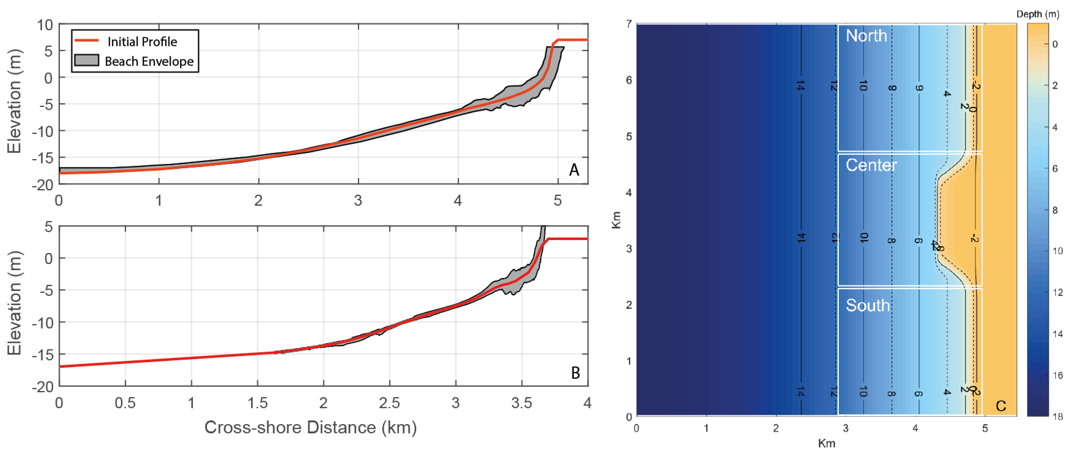
2.3.2. Initial Beach Profiles

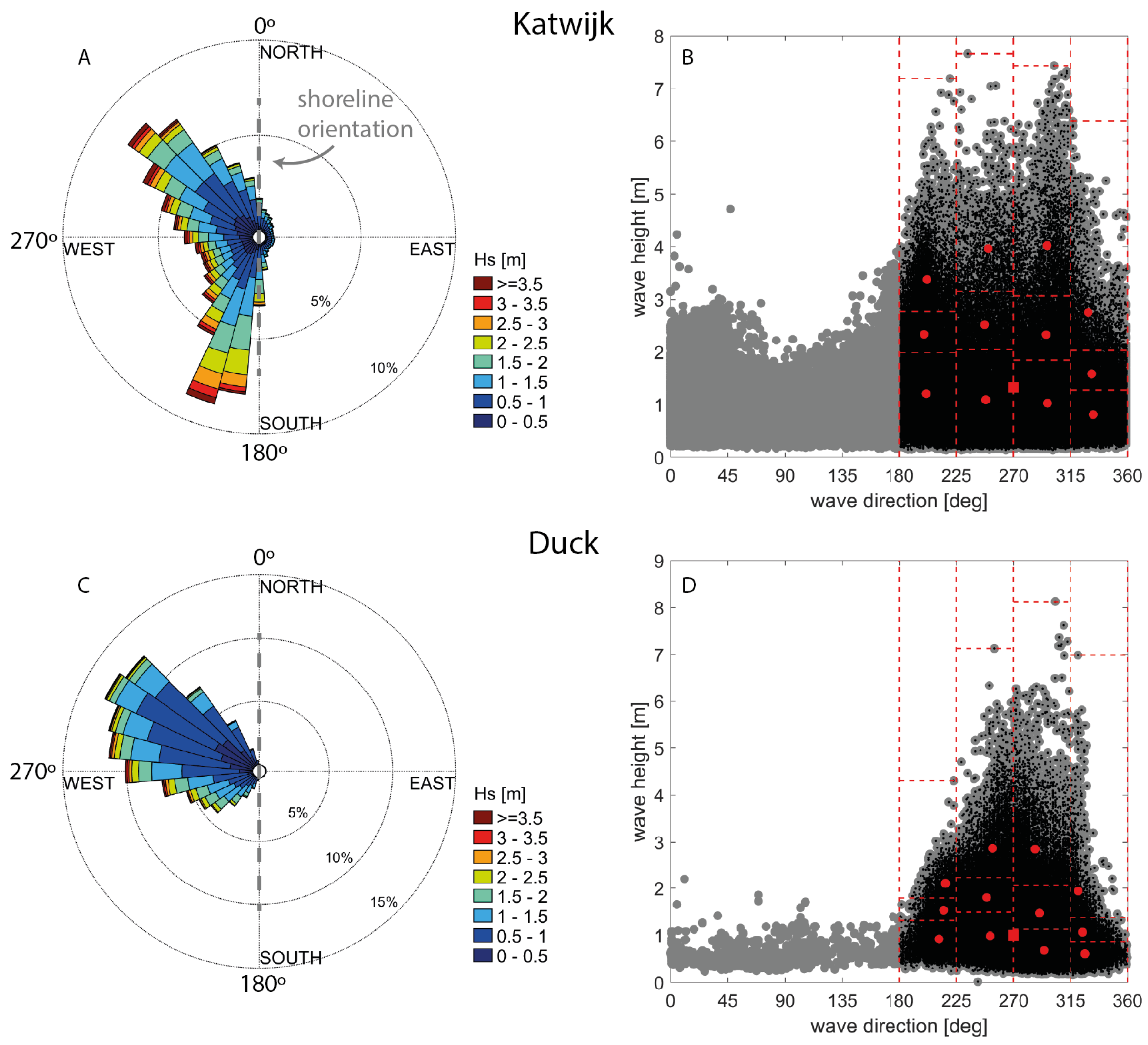
The initial bathymetry for the Dutch coast is a time-spatial averaged nearshore bed profile (Figure 1A) obtained from the Dutch JARKUS database [50] near Katwijk. The profiles were measured between 1965 and 2010 along 31 alongshore-distributed profiles covering 15 km of coastline from the dunes up to approximately 18 m depth. The average profile has a slope of 1V:185H up to 2.3 m depth, steepening to 1V:63H up to the mean water line. The sediment grain size composition varies between 200 and 350 $\mathsf{\mu }$m [5]. A comprehensive morpho-sedimentary description of the Dutch coast is presented in Wijnberg and Terwindt [51] and van Rijn [5]. Similarly, we averaged profiles from 1997 until 2008 (Figure 1B) at Duck situated north of the Field Research Facility Pier. The beach profile at Duck is steeper than at Katwijk. The average profile has a slope of 1V:120H up to 2.4 m depth, steepening to 1V:25H up to the mean water line. The sediment grain size varies between 125 and 250 $\mathsf{\mu }$m along most of the submerged profile with a second grain size mode of gravel-sized material near the shoreline [52]. An extensive site and data description for Duck is provided in Trowbridge and Young [53] and Gallagher et al. [54]. As can be seen in Figure 1B, the profile was linearly extended from 15 m depth up to the 17 m contour from where the wave data was retrieved. The cross-shore profile covers approximately 5 km at Katwijk and 3.8 km at Duck. From the measured envelopes in Figure 1, most morphological activity is constrained between the dunes and the 6 m depth contour at both sites.

The averaged profiles were extended seven kilometers in the alongshore direction creating an initial alongshore uniform bathymetry that suppresses alongshore gradients for the area 2DH models. To study effects of the wave parameterization on alongshore direction, a 3.7 Mm${}^3$ coastal hump was included in further simulations in the Katwijk model setup (Figure 1C; scenario 6). The hump resembles a beach nourishment extending from the dry beach up to approximately 5 m depth. For analysis, the nearshore area is divided into three sections: The central area corresponds to the hump and the other two are the adjacent coasts to the North and South. The computed volumes considered all areas extending from the dry beach into approximately 12 meter depth contour, enclosing the active beach profile, and therefore the majority of the sediment exchange happens via alongshore transport.

2.3.3. Wave Climate

The wave conditions for the Dutch Coast were recorded by the IJmuiden ‘Munitiestortplaats’ directional buoy in the North Sea between 1990 and 2016. The wave measurements from Duck were recorded by a wave rider buoy (station wvrdr630) from 1997 to 2018. The wave directions were rotated 30° at Katwijk and 161° at Duck, respectively, to realign the waves with our idealized coast based on the local shoreline orientation (Figure 2A,C). Therefore wave directions will be given in this new frame of reference, with 270° implying shore-normal wave incidence.

The wave climate at Katwijk consist of short period waves averaging 4.6 s with 11.7 s maximum. The maximum wave height reaches 7.6 m while the average is 1.32 m. The wave direction has two main components from SW (200°) and NW (310°) but also has a significant frequency of parallel and offshore going waves for 13% of the year. Duck has longer period waves up to 25 s and an average of 8.7 s. The maximum wave height reaches 8.12 m, averaging 0.99 m. The direction has one mode from 300° and limited offshore and parallel going waves summing 1% of the year.

For optimizing computational effort, the original time series were reduced into 13 representative waves following Walstra et al. [55] and Benedet et al. [56]. The wave reduction consisted of four directions and three heights plus an average wave condition to replace the duration of offshore and parallel directed waves. The representative wave conditions were obtained by dividing the wave climate into 12 bins of equal energy E, being $E\sim H_s^2$. Then, the average wave period, direction and the total duration were calculated within each bin. Consequently, one wave condition energetically represents a range (Figure 2B,D), consisting of significant wave height, wave period, wave direction and duration. The reduced wave climate for Katwijk and Duck is shown in Table 2, with condition number 7 being the averaged condition to replace the recorded offshore and parallel going waves.

The 13 reduced wave conditions were organized as a constant alternating time-series sequence, following the order from Table 2, changing every hydrodynamic hour until its duration was exhausted. In this approach we are constantly changing the wave energy followed by wave direction. While the ordering of wave conditions is known to affect the dynamics of surfzone bars [13,55], the present focus is on equilibrium morphology and large scale sediment transport behaviour. This alternation process ensures that no wave condition perpetuates for too long driving the morphology into an alternative equilibrium.

2.3.4. General Model Configurations

The numerical simulations are depth-averaged 2DH models with cross-shore resolution varying from 50 m offshore to 12.5 m towards the coastline and 50 m on the alongshore direction. The hydrodynamics are coupled with wave conditions computed with SWAN as online communication of bathymetry, waves, currents and water level. In combination with waves, the hydrodynamics for sediment transport are solved in Generalized Lagrangian Mean (GLM) mode to account for wave-induced processes, e.g., Stoke’s drift [43].

The propagated wave conditions were coupled with flow every 30 min in order to consider the wave–current interaction, wave-induced currents, water level fluctuations due to tides and morphological bed evolution. Based on available tidal records, the tidal water level amplitude was set to 1.0 m at Katwijk and 0.5 m for Duck, both as 12 h harmonic tides. To avoid undesired boundary effects, the alongshore domain encloses a 7 km long coastline with null gradient Neumann boundary conditions at the cross-shore boundaries.

After sensitivity analysis, not shown here, a constant morphological acceleration factor (morfac) between 10 and 20 was used to speed up the simulations performing in total 10 morphological years. The simulations 3 and 9 were performed with morfac equal to 10; the hump scenarios with morfac equal to 12; and models 4–6 and 10 with morfac equal to 20. These morfac values are similar to those used in other studies (e.g., [22,27,37]). Sediment transport was limited to depths great than 0.3 m at Katwijk and 0.4 m at Duck based on the non-dimensional wave period condition $T_p\sqrt{g/h}<40$, following Ruessink et al. [15], to exclude swash zone processes. A single sand fraction of 250 $\mathsf{\mu }$m was applied in all model runs. Other model settings are specified in the Supplementary material.

3. Results

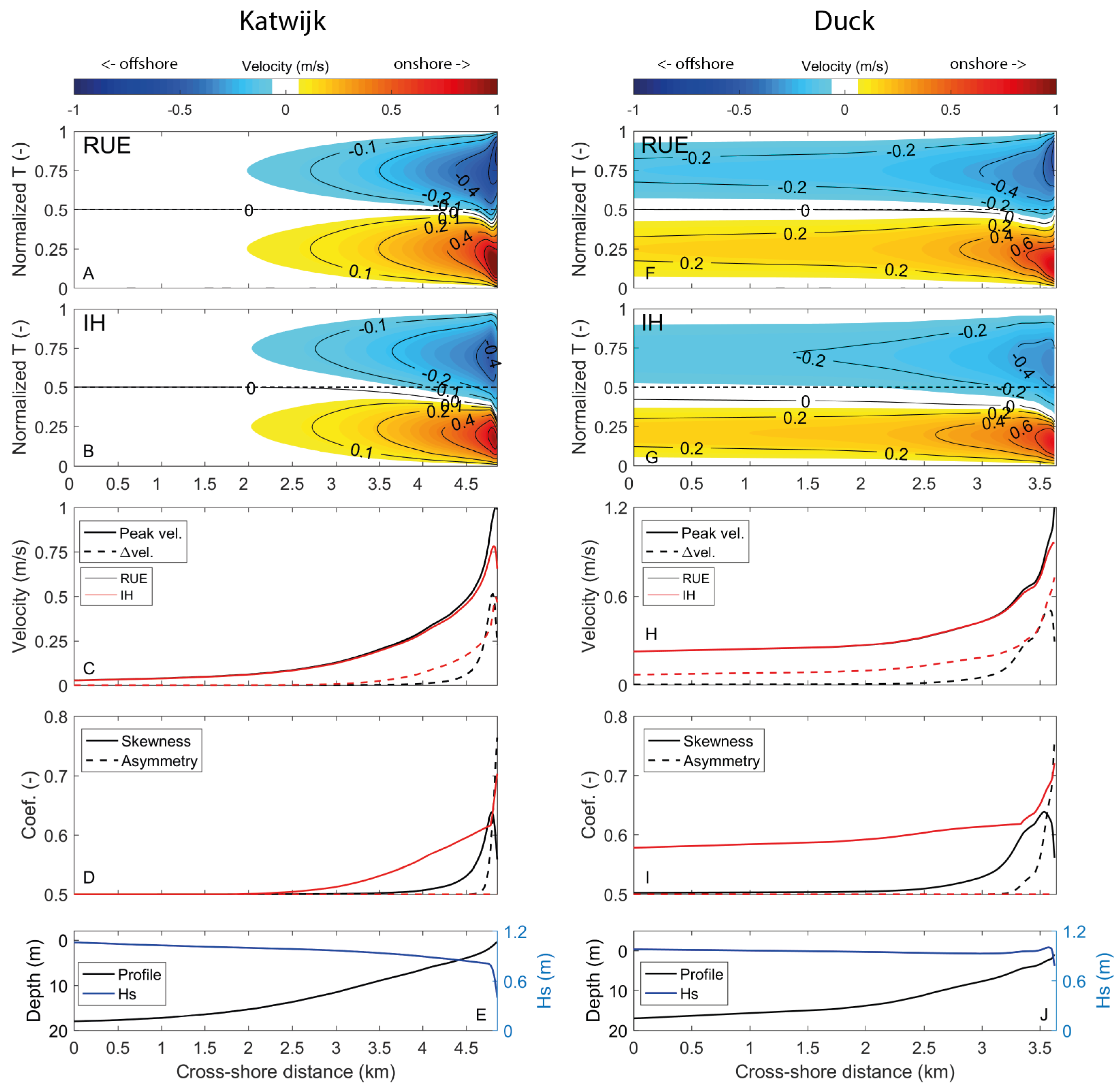
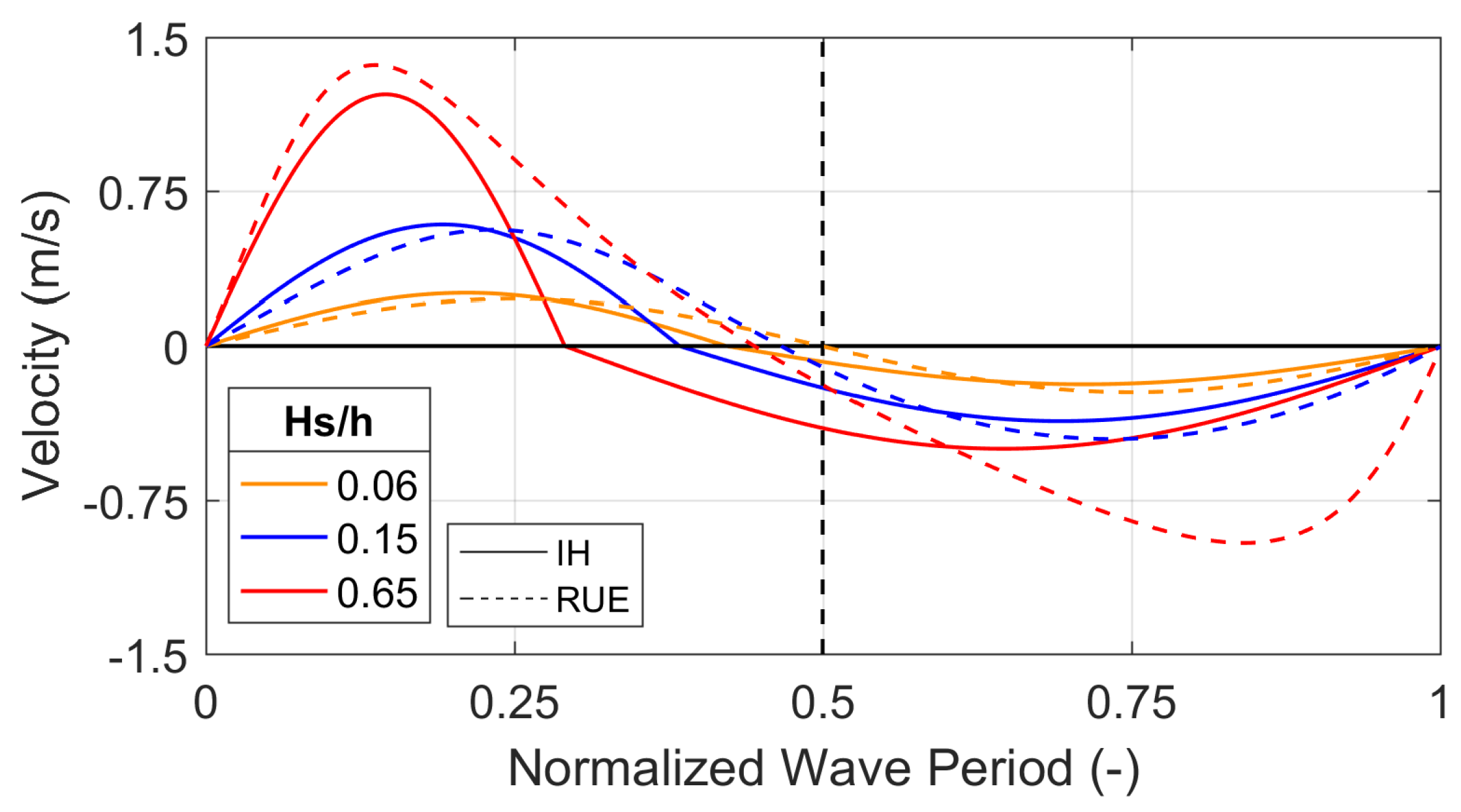
3.1. Cross-Shore Orbital Velocities

The cross-shore distribution of orbital velocities predicted with RUE and IH over the Katwijk and Duck profiles are shown in Figure 3A,B,F,G for the average wave condition (scenarios 1 and 7 in Table 1; wave 7 in Table 2). IH does not explicitly computes $Sk$ and $As$, then for direct comparison between methods we computed skewness ($R_u$) and asymmetry ($R_a$) coefficients based on velocity and acceleration, respectively (see Equation (1)). Here IH consistently predicts higher skewness than RUE, and also predicts skewness in deeper water (Figure 3D,I). For example, the skewness at Katwijk starts around 14 m depth for IH and 8 m for RUE. This effect is more pronounced at Duck where the wave period is larger. At Duck, IH is already skewed from the seaward boundary, at 17 m depth contour, while RUE shows linear behaviour up to 14.5 m depth. RUE predicts lower values of skewness seaward of the surfzone and develops asymmetry towards the surfzone, corresponding to 3 m depth at Katwijk and 6 m at Duck. The interval asymmetry exceeds skewness correspond with the zone of wave breaking at 1.5 m and 2.5 m depth at Katwijk and Duck, respectively (Figure 3E,J). On the other hand, IH has skewness-only, which increases strongly towards the waterline.

The main effects of the skewness predicted with IH into the orbital velocities and wave shape are twofold: (1) lower offshore-directed velocities in comparison with the onshore velocities and (2) the shorter crest period marked by the zero contour line deviating from half of normalized wave period. For RUE the sinusoidal linear shape persists longer towards the shoreline so that the onshore and offshore peak velocities are of similar magnitudes, deviating when skewness develops during shoaling process and again become nearly equal when asymmetry develops in the surfzone (Figure 3C,H). The peak onshore velocity is similar for both methods except in the very shallow areas where RUE predicts higher magnitudes. This means that the onshore velocities are similar for IH and RUE and the lower prediction of offshore velocities by IH is the main difference concerning the peak velocities.

These effects result from how IH translates the non-linearity into the orbital wave shape. After computing the peak onshore and offshore velocities the wave period is split artificially based on the ratio between ($u_{on}$) and ($u_{off}$). The intra-wave velocity is then computed separately for each direction with a sine expression (Equation (2)). This leads to a discontinuous wave shape for the intra-wave orbital velocity (Figure 4). As a consequence, IH produces larger skewness than RUE, especially for longer period waves as demonstrated in Figure 3 at Duck.

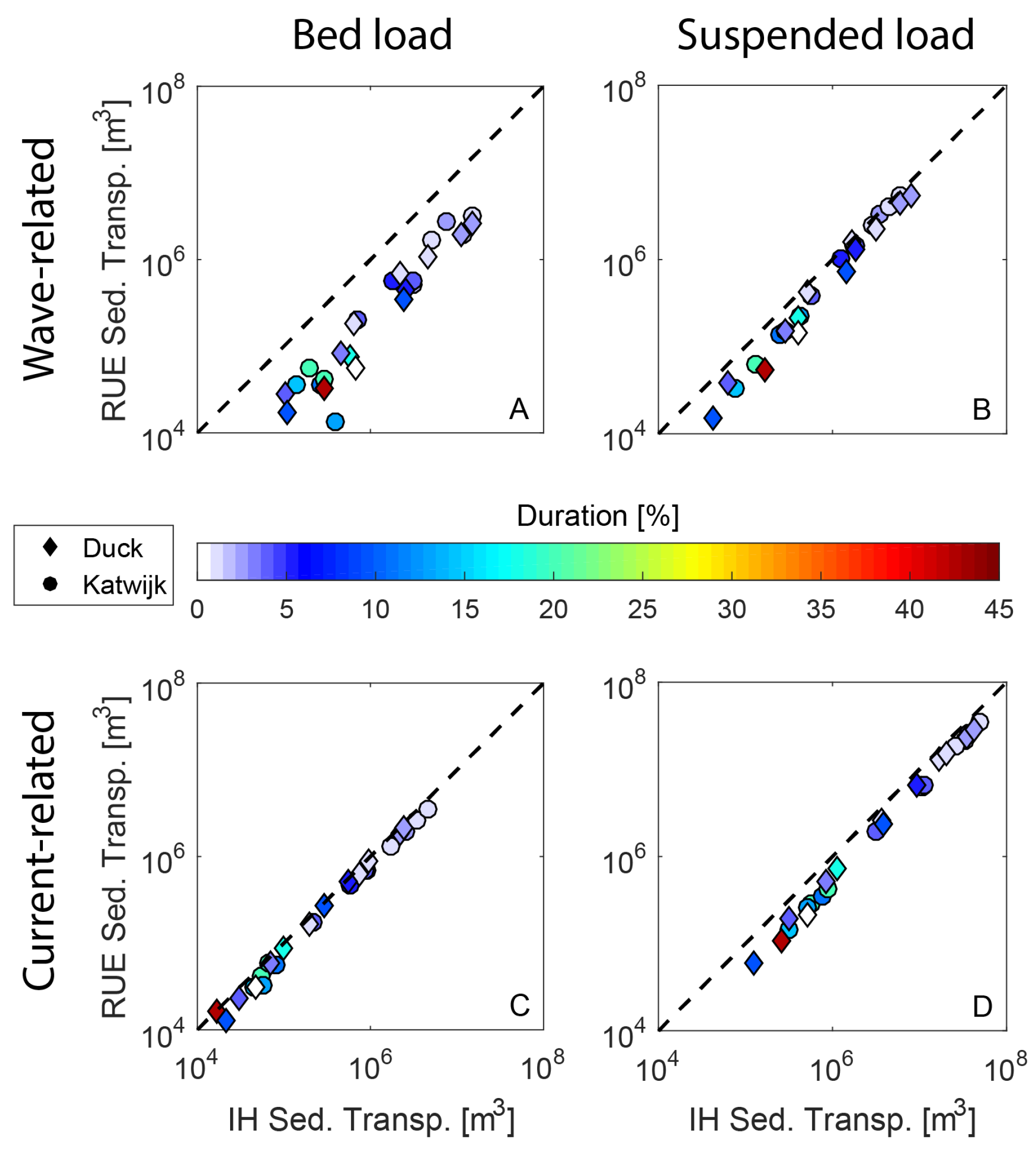
3.2. Sediment Transport on Alongshore Uniform Coasts

The orbital velocities are coupled to VR04 sediment transport via combined current and wave bed-shear stress. For the wave-related bed (Equation (4)) and suspended load (Equation (5)), the difference between onshore and offshore velocities is the main driver of cross-shore sediment transport and therefore we consider VR04 a skewness-based sediment transport predictor. For the bed load component, the critical shear stress enhances the non-linear behaviour in sediment transport near the beginning of motion due to the division of excess bed-shear stress by the critical shear stress.

Thus, the relation between flow velocity and sediment transport, in addition of critical shear stress of motion, creates a rather complex relation when adding non-linear oscillatory wave processes. To unravel this phenomena, Figure 5 compares the results of sediment transport (combined cross-shore and alongshore) between IH and RUE for each wave condition from Table 2 integrated over a tidal cycle. All IH simulations predicted more sediment transport than RUE. The sediment transport factor, defined as IH/RUE, varies from 1 to 3.1, except for the wave-related bed load transport ranging from approximately 3 to 12 with an outlier of 29. In general, the largest deviations between methods derive from small sediment transport values associated with low-energy frequent-duration wave conditions, specially for the wave-related bed load (Figure 5A). To reinforce this trend, the observed outlier corresponds to the average wave condition at Katwijk ($Hs=1.32$ m; $Tp=4.6$ s) due to a relatively large difference in transport magnitude while the absolute values were small ($1.08\times {10}^{-4}$ m${}^3$ for IH and $3.72\times {10}^{-6}$ m${}^3$ for RUE). Therefore, the largest discrepancies between methods derived from situations near the beginning of motion instead of from more energetic (stormy) wave conditions. As these low energetic conditions are predominant in the yearly wave climate, they may result in large deviations for the annual sediment budget.

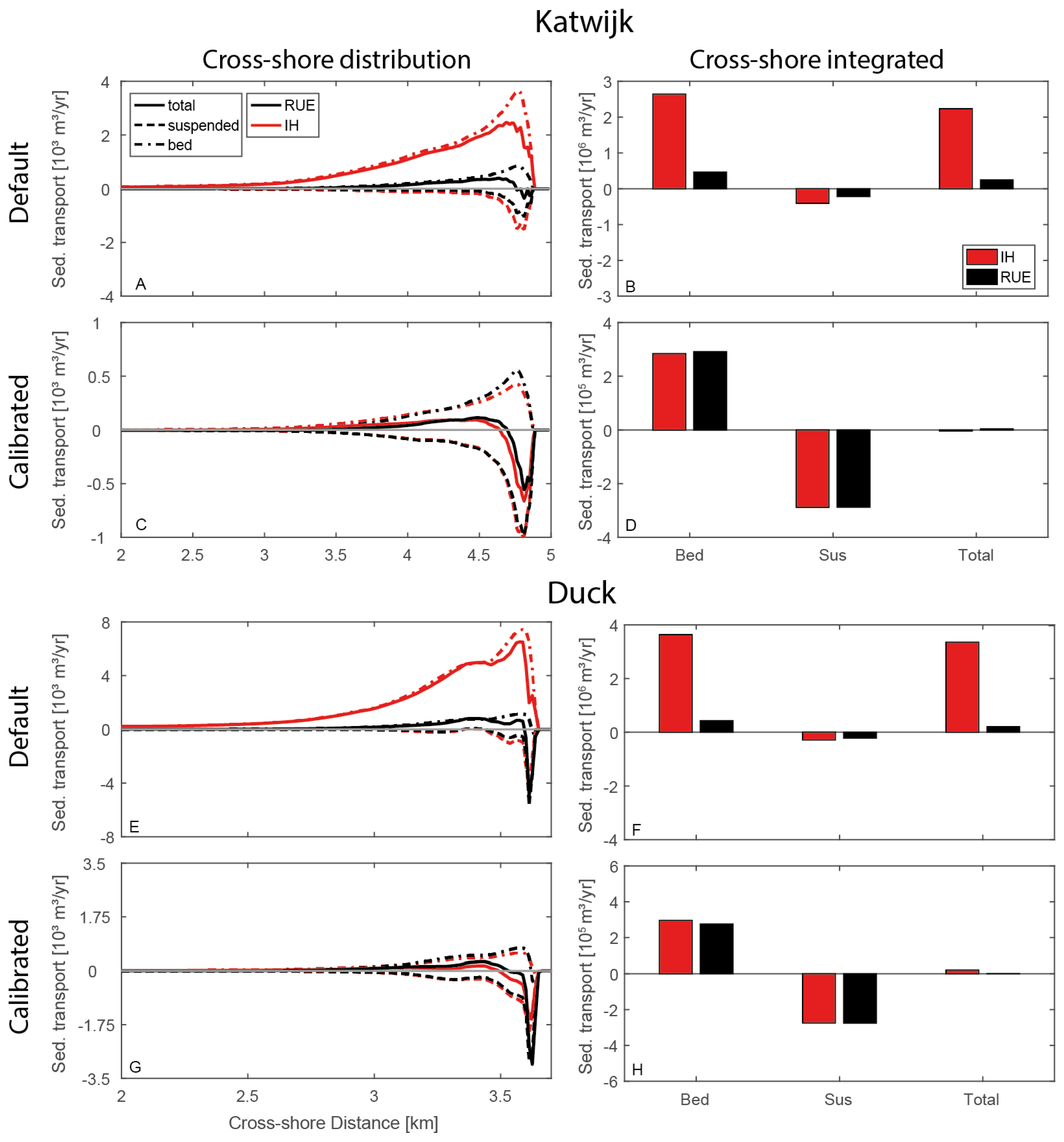
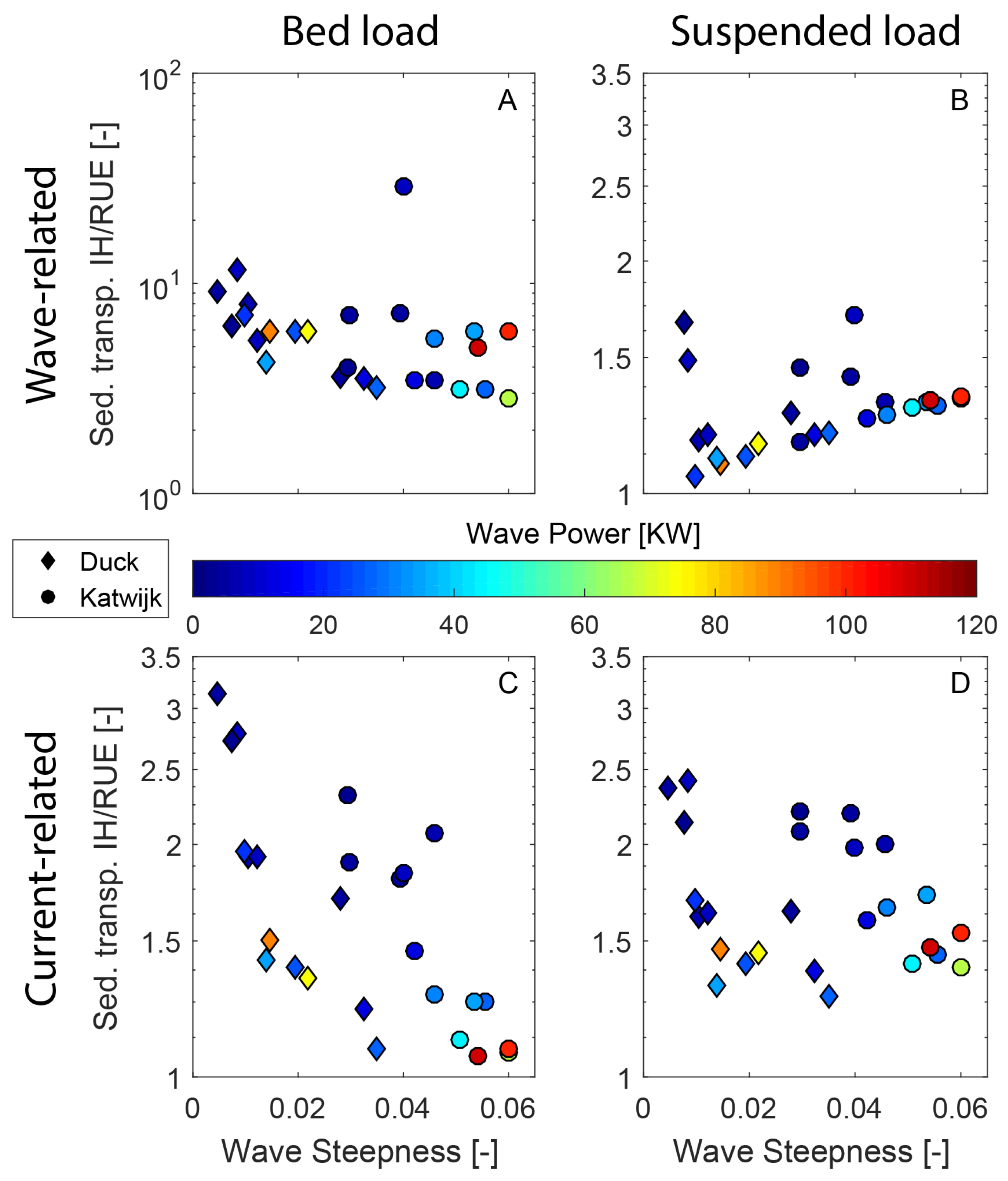
3.2.1. Cross-Shore Sediment Transport

Next we computed the annual equivalent cross-shore sediment transport (scenarios 2 and 8 in Table 1) on the alongshore uniform coast applying the reduced wave climate at Katwijk and Duck. First we computed the annual bed load, suspended load and total transport of default sediment transport factors (Figure 6A,B,E,F) and afterwards we defined calibration factors (Figure 6C,D,G,H and

Table 3. Sediment transport calibration factors for Katwijk and Duck for IH and RUE formulation. w stands for wave-related; c for current-related; b for bed load; and s for suspended load.

	Calibration Katwijk		Calibration Duck
	IH	RUE	IH	RUE
$F_{w,b}$	0.155	0.720	0.112	0.720
$F_{w,s}$	0.154	0.200	0.123	0.199
$F_{c,b}$	0.709	1.000	0.875	1.000
$F_{c,s}$	0.272	0.375	0.228	0.360

) aiming stable nearshore cross-shore profile for the morphological simulations.

At both sites, with default sediment transport settings, the net cross-shore annual bed load (combined of current and wave) is onshore-directed while the suspended load is offshore-directed. As individual components, not shown here, the wave-related bed load ($S_{w,b}$) and suspended load ($S_{w,s}$) transports are onshore-directed while the current-related bed load ($S_{c,b}$) and suspended load ($S_{c,s}$) are offshore-directed. The IH simulations shows higher magnitudes for all sediment transport components. The higher onshore-directed bed load leads to an onshore-offshore sediment budget imbalance, which in this case will result in large shoreline accretion, mainly caused by the wave-related bed load component (Figure 6B,F). The annual cross-shore-integrated wave-related bed load transport is 4.62 times higher in IH than in RUE for Katwijk and 6.37 times higher for Duck. The wave-related suspended load is a factor of 1.29 and 1.64 higher for Katwijk and Duck, respectively. The choice of orbital velocity parameterization also affects the current-related transports through the computation of sediment concentration from the combined wave–current shear stress; the current-related bed load was 1.41 times higher and the suspended load 1.37 times higher. After combining the four transport components, the total net cross-shore transport is onshore-directed by a factor of 4.8 higher in IH than RUE at Katwijk and 7.8 at Duck.

Based on the annually cross-shore-integrated sediment transport differences between IH and RUE, we performed a sediment transport calibration to be applied on the morphological models in addition of default value scenarios. Recapping, with this calibration procedure we want to achieve nearshore profile stability, with minimum shoreline translation, and equal total net cross-shore sediment transport between IH and RUE. First, we target the net total cross-shore transport to be zero for each method (i.e., IH and RUE). We started keeping the current-related bed load of RUE equal to one, as it computes the least transport magnitudes (Figure 5C), followed by correcting the wave-related bed load, wave-related suspended load and finally the current-related suspended load. This first iteration achieves the onshore-offshore balance of sediment and a second iteration was made to match the annual total transport between IH and RUE. Applying those calibration factors (see Table 3) resulted in equal annual cross-shore-integrated magnitudes of bed load and suspended load with net total load nearly zero (Figure 6D,H). Based on the necessary calibration factor to correct sediment transport, the largest differences are found in the wave-related bed load sediment transport, so that the $F_{w,b}$ was reduced to 11.2% and 15.5% of the original magnitude for IH at Duck and Katwijk, while RUE was kept at 72%. The $F_{w,s}$ was similarly reduced around 20% as the wave-related suspended load does not fully account for the intra-wave sediment transport and actually has similar behaviour in direction and magnitude as the wave-related bed load. Finally the $F_{c,s}$ was reduced between 23% and 37% to close the cross-shore sediment budget. After calibration, the cross-shore distribution of sediment transport shows similar shapes and gradients (Figure 6C,G), except in the shallowest areas where we showed deviations starting from the hydrodynamics (Figure 3). Therefore, local morphological variations are expected along the profile, especially in the surfzone and intertidal areas.

3.2.2. Alongshore Sediment Transport

The alongshore-directed sediment transport rates were analyzed for Katwijk, only, in order to provide insights on the hump evolution simulated with the same settings. Both IH and RUE methods predict net northward sediment transport at Katwijk. For default sediment transport settings IH and RUE predict 1,320,000 m³/year and 915,000 m³/year (Figure 7A,B). Thus, IH predicts 405,000 m³/year (that is 1.44 times) more net northward sediment transport compared to RUE. The bed load sediment transport factors for waves and currents are 2.0–2.1 and the suspended loads 1.0–1.3. However, after applying the cross-shore based calibration (Table 3), IH results in much lower values for the net alongshore transport, namely 73% of reduction from the default value; and 56% of reduction for RUE (Figure 7C,D). In volume, that represents a reduction of 968,200 m³/year for IH after calibration while for RUE 517,000 m³/year. This means that the sediment transport calibration aiming coastal stability forces changes in the alongshore sediment transport with more than a factor of two for IH and slightly higher for RUE. This reduction of littoral drift may affect long-term morphological development, and the timescale thereof, along non-uniform coasts.

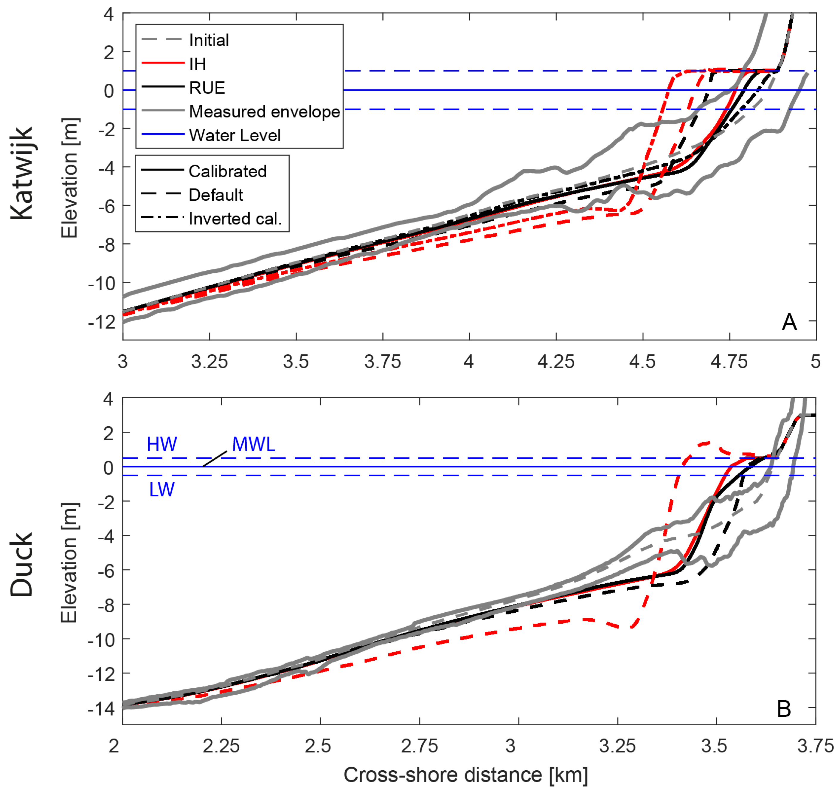
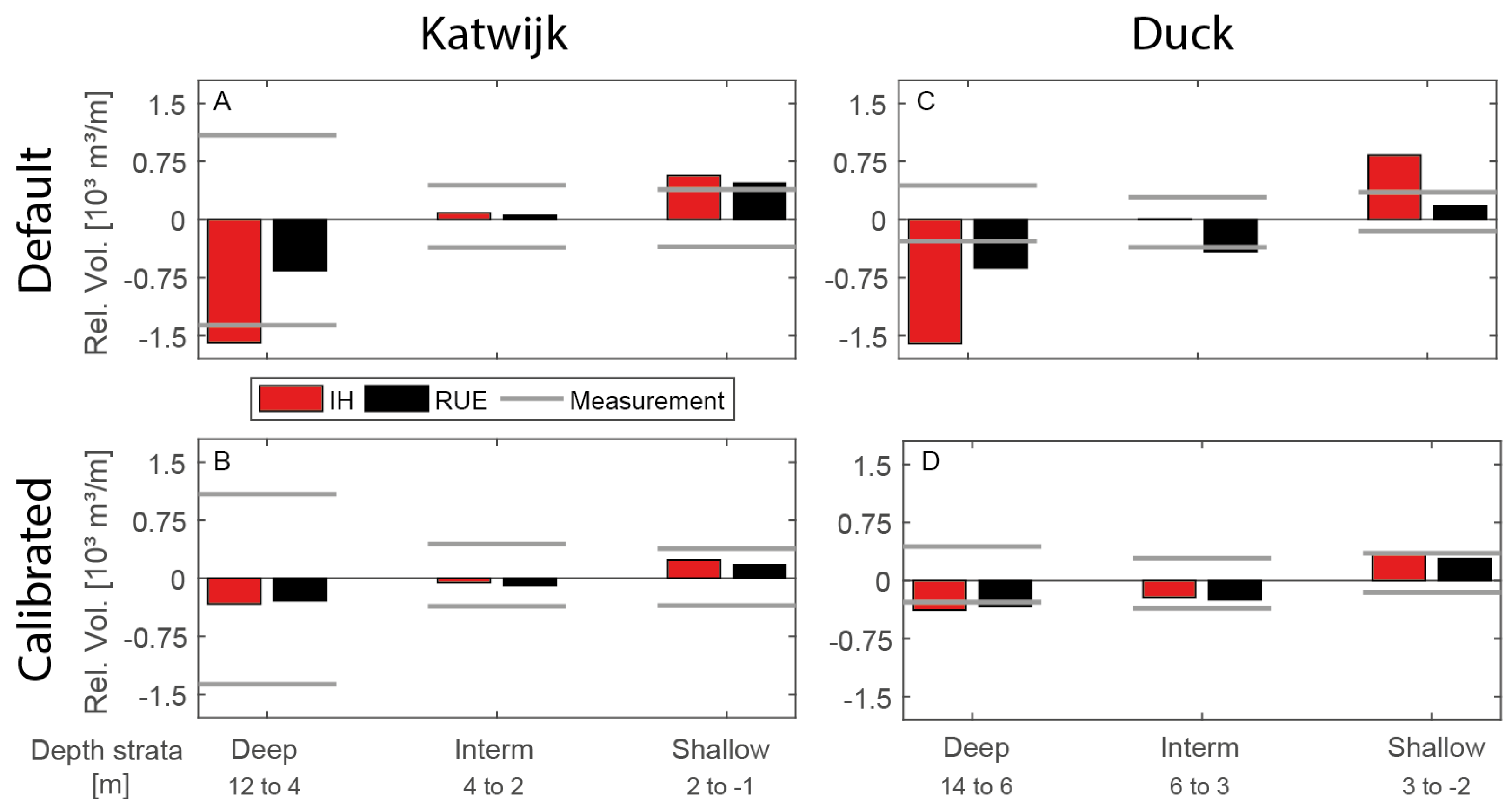
3.3. Alongshore Uniform Coastal Morphology

Ten morphological years of simulation were performed with default and calibrated transport factors (Figure 8; scenarios 3, 4, 5, 9, 10 in Table 1). For the default sediment transport simulations at Katwijk, the wave-related transport appears from approximately 12 m depth upwards. Between 12 m and 5 m IH erodes the bed creating net onshore sediment transport. As a result, the shallower areas and the shoreline became excessively obese and steep. Simulations with RUE also show net onshore transport, though less than IH, but hardly eroding deeper areas. In comparison to the measured bed profile envelope, IH prediction is outside the envelope from 9 m depth up to the shoreline while RUE deviates only around the intertidal zone. From the measured profile envelopes we expected most morphological dynamics happening from 6 m up to the shoreline, therefore, especially IH overestimated the profile changes.

Following calibration, both IH and RUE stayed within the envelope boundaries, with IH showing slightly more deposition in the intertidal shallow area. In addition, the calibration succeeded in balancing the onshore and offshore transport magnitudes towards a stable profile with minimum shoreline translation. The scenarios with RUE factors applied in IH and vice-versa (inverted calibration, scenario 6) show the largest morphological deviations. The RUE simulation with IH factors has the closest fit with the initial (equilibrium) profile which, as a first glance, suggests the best performance. However it is important to highlight that the extreme lower transport factors applied (see Table 3) for wave-related transport (around 10–15%) just shows lower morphological dynamics rather than being the best calibration. On the other hand, IH with RUE predicts the largest shoreline displacement (i.e., 290 m) and large deposition on shallow waters up to 4 m depth. This extreme case is the combination of high onshore transport rates due to wave-related bed load in addition of the reduced offshore transport caused by the smaller factor on the current-related suspended load. Similar response was observed for Duck (Figure 8B) with a total shoreline displacement of 230 m with IH in comparison with 67 m with RUE for default scenarios. After calibration there is a divergence in the intertidal and subtidal areas up to 2 m depth where IH results in a larger deposit. At Duck both methods resulted in more erosion on the lower shoaling zone and deposition on the upper shoaling zone and surfzone.

Despite the parameterization choice and calibration factor, there is a general and alike steepening of the shoreface in all simulations, excepted when the wave-related transport was drastically reduced in the scenario of RUE with IH calibration factors.

The combined interpretation of default, calibrated and inverted calibration unravels: (1) the wave-orbital motion and its parameterization highly affects the sediment transport in the nearshore and consequently the morphological development in this area; and (2) how much the (wrong) calibration factors can affect the morphological development, especially for IH that predicts larger onshore transport and therefore is more sensitive to small changes in calibration factors. The wave-related sediment transport is the main driver of nearshore sediment transport, which promotes only onshore sediment transport for the 2DH configuration. This trend ultimately results in disproportional shoreline progradation, when the offshore-directed current-related transport cannot balance this onshore component, in addition of causing shoreface steepening. In this perspective, IH with larger (in our case 4.6–7.8 times higher) onshore transport is more sensitive and prone to calibration, implying that small inaccuracies in calibration factors result in large profile and shoreline translation.

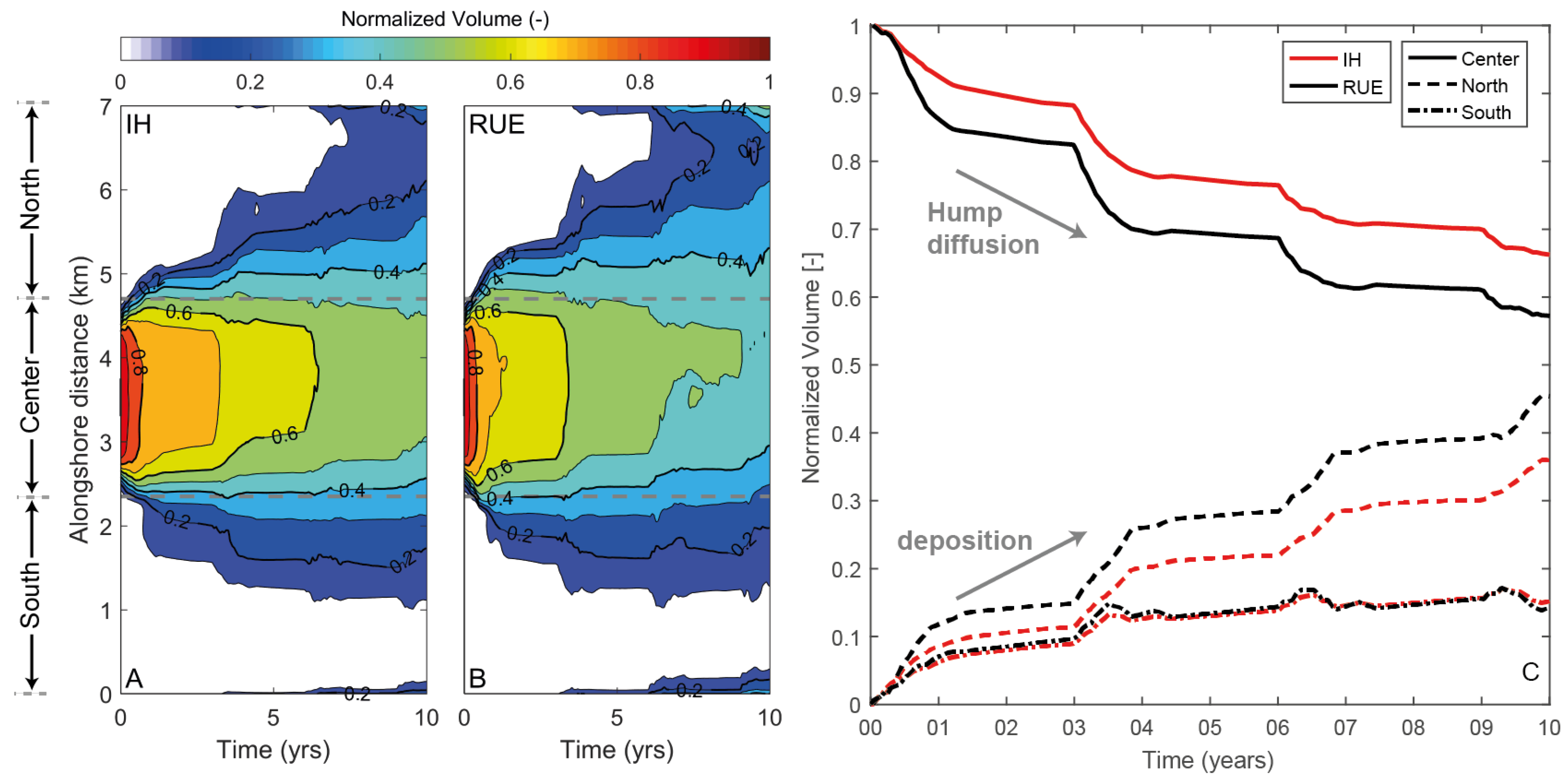
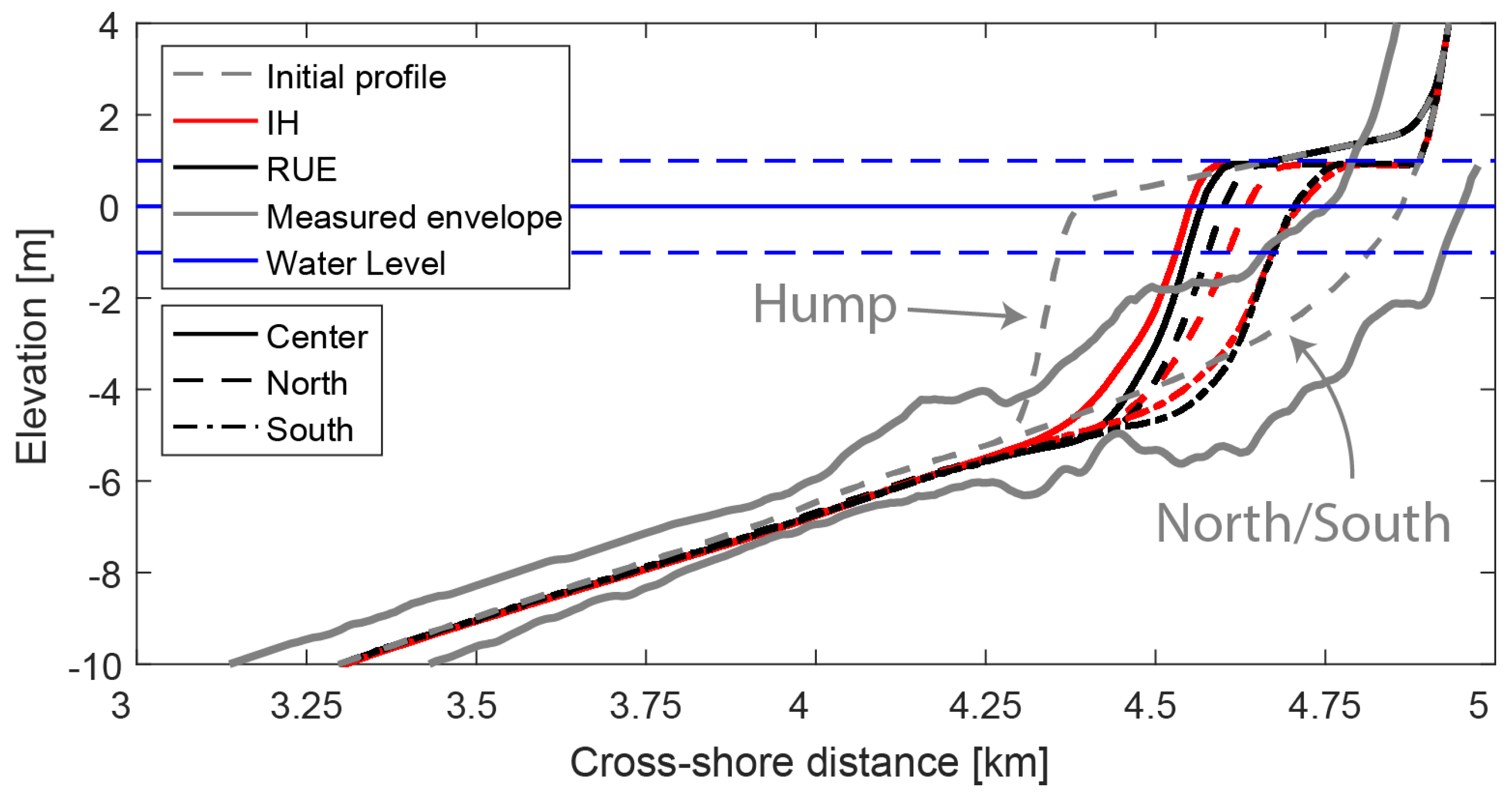
3.4. Alongshore Non-Uniform Coast Morphology—Coastal Hump

Finally, we performed morphological simulations with a ‘hump’ (scenario 6 in Table 1) using the calibrated factors (Table 3) in order to exclude, as much as possible, cross-shore effects (i.e., erosion and deposition leading to shoreline translation) that were already extensively described in the alongshore uniform coast setup. As can be seen in Figure 9, erosion and shoreline retreat is concentrated within the hump central area. Most hump sediment is transported and deposited in the North adjacent area while the South benefits less due to the northward net sediment trend (Figure 7).

The volumetric evolution follows pulses of fast diffusion when the more energetic waves occur in the time series followed by calmer period with slower decay (Figure 9). In the Center, RUE predicts faster loss of sediment in comparison with IH. After 10 years, the hump with RUE decayed to 57% from its initial volume of 3.7 Mm³ while IH decayed to 66%, representing a deviation of 336,400 m³ between the two methods.

The profile evolution after 10 years shows the retreat of the center profile, faster for RUE, while the North concomitantly responds with larger shoreline progradation when compared to the South (Figure 10). In these scenarios, RUE predicts faster diffusion of the hump itself. This means, for example, that a beach nourishment would feed the adjacent downdrift areas faster, while lasting shorter, in comparison with IH predictions. Therefore, the parameterization choice affects the timescale of alongshore morphological processes. In general, the profiles evolved towards the measured envelope in a trend to restore the alongshore uniform dynamic equilibrium when the alongshore transport gradients tend to zero. Despite the introduction of this large shoreline perturbation, the final cross-shore profile (Figure 10) did not differ in shape from the alongshore uniform case (Figure 8A), which is a further indication that the final morphology is indeed a robust equilibrium condition for the chosen wave climate, calibration and orbital velocity parameterization.

4. Discussion

The near-bed orbital velocities parameterizations differ in predicting wave shape transformation in shallow water and profoundly impact the resulting long-term sediment transport and morphological evolution. Below we discuss the main implication of parameterization choice.

4.1. Long-Term Morphodynamic Evolution

The main consequences of higher onshore-directed sediment transport by IH are twofold: (1) erosion of deeper nearshore areas where waves were not expected and observed to cause such effect (Figure 8 and Figure 11) and (2) overfeed of the shallow upper beach profile. Here, the first effect was caused by non-linearities (skewness) starting earlier (deeper) in the wave propagation path (Figure 3) resulting in a onshore-directed gradient that pushes the sediment towards the shoreline (Figure 6). This phenomena combined with incorrectly increasing skewness in the surfzone (Figure 3) results in larger shoreline progradation (Figure 8) due to excessive deposition, beyond the measured profiles and volumes, and imbalance between onshore and offshore-directed transport (Figure 6 and Figure 11). This excess of onshore sediment transport was larger for the longer period waves of Duck, reaching a factor of 7.8 when considering the annual sediment budget, which translated into unrealistic shoreline progradation and profile evolution (Figure 8B). With default settings, RUE parameterization also overestimated onshore transport, however to less extent in comparison with IH.

The main reason for unrealistic net onshore sediment transport is the combination of the wave shape parameterization and the importance of the threshold for the beginning of sediment motion in the lowest wave classes. The skewness-only IH method predicts larger skewness and sediment transport in comparison with the skewness-asymmetry RUE predictor. The higher sediment transport factors (i.e., IH/RUE), especially for the wave-related bed load component, correlates with lower steepness and low energy waves (Figure 12), including the outlier (i.e., factor of 29) represented by the average wave condition of Katwijk. In Figure 12 we defined wave power as $Power={\displaystyle \frac{\rho g^2{H}_s^2{T}_p}{32\pi }}$ in Watts and wave steepness as $Steepness=H_s/L$. The largest discrepancies between the two methods thus derive from situations near the beginning of motion for the bed load component (Equation (4)) when the sediment transport is strongly non-linear, in this case, higher than a power of 3 for VR04. These low energetic conditions have a larger duration (Figure 5) in comparison with the high-energy stormy events and are the dominant wave conditions in the wave climate (Table 2). Therefore, one can expect sediment transport deviations within a factor of 3–12 when simulating morphology with a wave climate or even higher when including an individual wave condition only, which is commonly of small–intermediate wave energy (e.g., [22,23,30,32,33,34,35,36,37]).

After applying calibration factors on the sediment transport, the overall equilibrium profiles and volume changes with IH and RUE were fairly similar (Figure 8 and Figure 11). Nonetheless there are discrepancies in deeper and especially shallower areas. The overfeeding near the shoreline was also observed for other skewness parameterizations methods in cross-shore models (e.g., [12,15,17]). Meanwhile, the shoaling zone, where skewness dominates, showed closer results. However, to achieve these conditions, the wave-related sediment transport for IH had to be reduced to 10–15% from the default values. Such reduction, although extreme, is not an exception when compared to recent studies [23,27,37], which raises serious doubts about the validity of IH to coastal environment applications in combination with general sediment transport predictors (e.g., [44,45,57]). Based on the assumption that 2DH models have to compensate for the lack of offshore-directed transport, with IH we are implicitly considering that 85–90% of transport is offshore-directed due to return currents, for example. On the other hand, with RUE, when we applied a correction of 70%, we are compensating for 30% of offshore-directed transport. The latter figure better represents an average condition between calm and storm conditions, while the 85–90% of IH represents storm conditions when undertow is dominant over short-wave non-linearity [7,12,54].

The main adverse consequence of (over)compensating the sediment transport aiming to counteract shoreline translation is the drastic reduction of alongshore transport, in the order of 73% in our case with IH. This highlights the current limitations in properly reproducing overall morphology and time-scales in one model. Reducing the net alongshore transport by a factor of 0.73 (i.e., 968,000 m³/year) represents 385% of the annual net alongshore transport computed by van Rijn [5], based on 200,000 m³/year estimation for the central Dutch Coast. This means that in applications of IH, one could either realistically simulate the alongshore process or the cross-shore process but not the combination. This limitation further hampers the hindcast and forecast of more complex environments, like tidal basins and inlets which work in strict balance and feedback between waves, tides and fluvial processes in three dimensions.

4.2. Limitations and Perspectives for Wave-Driven Sediment Transport Prediction

Yet our results derive from the Delft3D model, we believe that the RUE parameterization would also improve other morphodynamic numerical models, not restricted to 2DH applications, as it corrects a fundamental mismatch in wave hydrodynamics, which is common to other 1D-2DHV-3D morphodynamic models. Skewness-only parameterizations proved to be able to reproduce beach recovery, after storms, in specific cross-shore 1D/2DV models (see compilation in [12]). However, as demonstrated in Dubarbier et al. [17], the performance near the shoreline is the result of overcompensation of skewness-related transport, which has been used in the past to compensate for the lack of asymmetry effects in sediment transport functions. Here we observed a similar issue in the comparison of hydro-morphological results with IH versus RUE in a model-to-model approach and validation of results with measured beach-envelopes. Therefore, it is relevant to consider the origin and physical basis of each parameterization. RUE derived from nearshore field measurements, including the Central Dutch and Duck coasts [18], while IH and its further adaptations were based on scaled lab experiments [10,16] intended to reproduce wave-skewness. Therefore, we can argue that RUE provides better estimations of near-bed orbital velocities than IH, especially for our case-studies in Katwijk and Duck as shown by our hydrodynamic and morphological results. The important improvement is that these effects need no longer to be compensated by extreme calibration factors on the sediment transport, which affects alongshore transport as well, but addresses the hydrodynamics of orbital velocities. Consequently, the approach in this paper is suitable for large-scale, long-term 2DH modelling but still limited for predicting coastal beach profiles, as all scenarios predict rather steep and convex shoreface profiles (Figure 8), which we attribute to the lack of (quasi)3D-vertical processes combined with the dominant onshore-directed sediment transport driven by waves, similarly to observations from van Rijn et al. [12] and Grunnet et al. [27].

The IH predictor overestimates sediment transport mainly for the wave-related bed load component (Figure 6 and Figure 12). A consequence is that, IH also promotes morphological diffusion due to bed slope gravitational effects. The bed slope effects on sediment transport and morphological development strongly determine the results for situations with currents-only as demonstrated in Baar et al. [58,59]. With the overestimated bed load contribution of waves, we expect stronger diffusion affecting the very shallow areas represented by shoals, bars and channels. The down-slope transport acts as a natural damping mechanism of morphological perturbations, however, its overprediction leads to unnaturally flat morphology. This damping effect was also explored by Dubarbier et al. [17,60] for nearshore sandbars where increasing the downslope transport component decreased the growth of nearshore sandbars in their model.

The results generalize to many models and general sediment transport predictors that do not account for asymmetry-driven sediment transport (e.g., [43,45,61]). On the other hand, specialist, coastal-oriented sediment transport predictors such as Dubarbier et al. [17] and van Thiel de Vries [62] incorporated asymmetry-driven sediment transport, but these are strongly dependent on user-defined calibration due to the lack of a robust physical relation [63]. Moreover, such coastal-oriented formulations are poorly tested and arguably unsuitable for fluvial processes that are important in the fluvial-tidal transition that the general transport predictors can cover. Thus, further research should focus on robust incorporation of asymmetry-driven sediment transport into general and broadly applicable morphodynamic models, while the present advance opens up the possibility of long-term morphological modelling of coastal systems where cross-shore and alongshore transport are of similar importance.

5. Conclusions

The parameterization of wave-induced near-bed orbital velocities highly affects the long-term (year to decades) prediction of the nearshore morphology due to its non-linear relations with sediment transport. The comparison of the Isobe Horikawa (IH) [10] skewness-only parameterization versus the skewness and asymmetry method of Ruessink (RUE) [18] within the Van Rijn (VR04) transport equations [43] shows that a better representation of wave shape and near-bed orbital velocities leads to overall more realistic morphodynamic predictions.

The IH parameterization predicts larger skewness and onshore-directed sediment transport in comparison with the RUE method. Depending on the wave condition, the tidally integrated net transport with IH was between 3 and 12 times larger than with RUE, with an outlier of 29. The largest differences were observed for calm wave conditions, which are dominant in the wave climate, further enhancing the difference between the two methods in the yearly sediment budget. Thus, with default sediment transport settings, IH simulations led to an overfeeding of shallow areas while eroding the deeper portion of the profile. RUE simulations with default settings also overpredict onshore-directed transport in the shoaling and surfzone, however, to a lesser extent. After applying calibration factors on the sediment transport components, to ensure shoreline stability by means of equal yearly net onshore and offshore sediment transport, both IH and RUE predicted profiles within measured beach envelopes at two sites selected, i.e., Duck, NC, USA and Katwijk, NL. However, IH wave-related sediment transport needed to be reduced to 10–15%, which in turn affected the alongshore transport rates by 73%, representing 385% of the annual littoral drift of the Dutch Coast. For the same conditions, RUE simulations were reduced to 72% in order to match the beach envelopes and consequently had a lower impact on the alongshore sediment transport (56%).

Thus, by improving the parameterization of near-bed wave orbital motion there is less need to (over-)calibrate sediment transport. The skewness-asymmetry parameterization also proved to be robust, in the sense that predictions were less sensitive to variations in the user-defined calibrations factors. Therefore, RUE parameterization results in a closer coupling of cross-shore and alongshore sediment transport in the nearshore, which improves the long-term hindcast and expectations related to complex coastal and estuarine environments.

References

1. Elgar, S.; Guza, R.T. Nonlinear model predictions of bispectra of shoaling surface gravity waves. J. Fluid Mech. 1986, 167, 1–18. [Google Scholar] [CrossRef]
2. Zijlema, M.; Stelling, G.; Smit, P. SWASH: An operational public domain code for simulating wave fields and rapidly varied flows in coastal waters. Coast. Eng. 2011, 58, 992–1012. [Google Scholar] [CrossRef]
3. Malej, M.; Mith, J.M.; Salgado-Dominguez, G. Introduction to Phase-Resolving Wave Modeling with FUNWAVE; ERDC/CHL CHETN-I-87; US Army Corps of Engineers: Washington, DC, USA, 2015.
4. Van der Spek, A.J.; Beets, D.J. Mid-Holocene evolution of a tidal basin in the western Netherlands: A model for future changes in the northern Netherlands under conditions of accelerated sea-level rise? Sediment. Geol. 1992, 80, 185–197. [Google Scholar] [CrossRef]
5. Van Rijn, L. Sand Budget and Coastline Changes of the Central Coast of Holland between Den Helder and Hoek van Holland, Period 1964–2040; Deltares: Delft, The Netherlands, 1995. [Google Scholar]
6. Beets, D.J.; van der Spek, A.J.F. The Holocene evolution of the barrier and the back-barrier basins of Belgium and the Netherlands as a function of late Weichselian morphology, relative sea-level rise and sediment supply. Neth. J. Geosci. 2000, 79, 3–16. [Google Scholar] [CrossRef] [Green Version]
7. Stive, M. A model for cross-shore sediment transport. In Proceedings of the 20th International Conference on Coastal Engineering, Taipei, Taiwan, 9–14 November 1986; pp. 1550–1564. [Google Scholar]
8. Dean, R.; Perlin, M. Intercomparison of near-bottom kinematics by several wave theories and field and laboratory data. Coast. Eng. 1986, 9, 399–437. [Google Scholar] [CrossRef]
9. Rienecker, M.M.; Fenton, J.D. A Fourier approximation method for steady water waves. J. Fluid Mech. 1981, 104, 119–137. [Google Scholar] [CrossRef]
10. Isobe, M.; Horikawa, K. Study on Water Particle Velocities of Shoaling and Breaking Waves. Coast. Eng. Jpn. 1982, 25, 109–123. [Google Scholar] [CrossRef]
11. Roelvink, J.; Brøker, I. Cross-shore profile models. Coast. Eng. 1993, 21, 163–191. [Google Scholar] [CrossRef]
12. Van Rijn, L.; Walstra, D.; Grasmeijer, B.; Sutherland, J.; Pan, S.; Sierra, J. The predictability of cross-shore bed evolution of sandy beaches at the time scale of storms and seasons using process-based Profile models. Coast. Eng. 2003, 47, 295–327. [Google Scholar] [CrossRef]
13. Walstra, D.; Reniers, A.; Ranasinghe, R.; Roelvink, J.; Ruessink, B. On bar growth and decay during interannual net offshore migration. Coast. Eng. 2012, 60, 190–200. [Google Scholar] [CrossRef]
14. Roelvink, J.; Stive, M. Bar-generating cross-shore flow mechnisms on a beach. J. Geophys. Res. Oceans 1989, 94, 4785–4800. [Google Scholar] [CrossRef]
15. Ruessink, B.G.; Kuriyama, Y.; Reniers, A.J.H.M.; Roelvink, J.A.; Walstra, D.J.R. Modeling cross-shore sandbar behavior on the timescale of weeks. J. Geophys. Res. Earth Surf. 2007, 112. [Google Scholar] [CrossRef] [Green Version]
16. Grasmeijer, B. Process-Based Cross-Shore Modeling of Barred Beaches. Ph.D. Thesis, Utrecht University, Utrecht, The Netherlands, 2002. [Google Scholar]
17. Dubarbier, B.; Castelle, B.; Marieu, V.; Ruessink, G. Process-based modeling of cross-shore sandbar behavior. Coast. Eng. 2015, 95, 35–50. [Google Scholar] [CrossRef]
18. Ruessink, B.; Ramaekers, G.; van Rijn, L. On the parameterization of the free-stream non-linear wave orbital motion in nearshore morphodynamic models. Coast. Eng. 2012, 65, 56–63. [Google Scholar] [CrossRef]
19. Warner, J.C.; Sherwood, C.R.; Signell, R.P.; Harris, C.K.; Arango, H.G. Development of a three-dimensional, regional, coupled wave, current, and sediment-transport model. Comput. Geosci. 2008, 34, 1284–1306. [Google Scholar] [CrossRef]
20. Villaret, C.; Hervouet, J.M.; Kopmann, R.; Merkel, U.; Davies, A.G. Morphodynamic modeling using the Telemac finite-element system. Comput. Geosci. 2013, 53, 105–113. [Google Scholar] [CrossRef]
21. Bertin, X.; Oliveira, A.; Fortunato, A.B. Simulating morphodynamics with unstructured grids: Description and validation of a modeling system for coastal applications. Ocean Modell. 2009, 28, 75–87. [Google Scholar] [CrossRef]
22. Nardin, W.; Fagherazzi, S. The effect of wind waves on the development of river mouth bars. Geophys. Res. Lett. 2012, 39. [Google Scholar] [CrossRef]
23. Nienhuis, J.H.; Ashton, A.D. Mechanics and rates of tidal inlet migration: Modeling and application to natural examples. J. Geophys. Res. Earth Surf. 2016, 121, 2118–2139. [Google Scholar] [CrossRef]
24. Luijendijk, A.P.; Ranasinghe, R.; de Schipper, M.A.; Huisman, B.A.; Swinkels, C.M.; Walstra, D.J.; Stive, M.J. The initial morphological response of the Sand Engine: A process-based modelling study. Coast. Eng. 2017, 119, 1–14. [Google Scholar] [CrossRef] [Green Version]
25. Nardin, W.; Fagherazzi, S. The Role of Waves, Shelf Slope, and Sediment Characteristics on the Development of Erosional Chenier Plains. Geophys. Res. Lett. 2018, 45, 8435–8444. [Google Scholar] [CrossRef]
26. Tonnon, P.; Huisman, B.; Stam, G.; van Rijn, L. Numerical modelling of erosion rates, life span and maintenance volumes of mega nourishments. Coast. Eng. 2018, 131, 51–69. [Google Scholar] [CrossRef] [Green Version]
27. Grunnet, N.M.; Walstra, D.J.R.; Ruessink, B. Process-based modelling of a shoreface nourishment. Coast. Eng. 2004, 51, 581–607. [Google Scholar] [CrossRef]
28. Briere, C.; Giardino, A.; van der Werf, J. Morphological modeling of bar dynamics with DELFT3D: the quest for optimal free parameter settings using an automatic calibration technique. Coast. Eng. Proc. 2011, 1, 60. [Google Scholar] [CrossRef]
29. Storms, J.E.A.; Stive, M.J.F.; Roelvink, D.J.A.; Walstra, D.J. Initial Morphologic and Stratigraphic Delta Evolution Related to Buoyant River Plumes. In Proceedings of the Coastal Sediments ’07, New Orleans, LA, USA, 13–17 May 2007. [Google Scholar] [CrossRef]
30. Edmonds, D.A.; Slingerland, R.L. Significant effect of sediment cohesion on delta morphology. Nat. Geosci. 2010, 3, 105–109. [Google Scholar] [CrossRef]
31. Guo, L.; van der Wegen, M.; Roelvink, D.J.; Wang, Z.B.; He, Q. Long-term, process-based morphodynamic modeling of a fluvio-deltaic system, part I: The role of river discharge. Cont. Shelf Res. 2015, 109, 95–111. [Google Scholar] [CrossRef]
32. Van der Vegt, H.; Storms, J.; Walstra, D.; Howes, N. Can bed load transport drive varying depositional behaviour in river delta environments? Sediment. Geol. 2016, 345, 19–32. [Google Scholar] [CrossRef] [Green Version]
33. Braat, L.; van Kessel, T.; Leuven, J.R.F.W.; Kleinhans, M.G. Effects of mud supply on large-scale estuary morphology and development over centuries to millennia. Earth Surf. Dyn. 2017, 5, 617–652. [Google Scholar] [CrossRef] [Green Version]
34. Geleynse, N.; Storms, J.E.; Walstra, D.J.R.; Jagers, H.A.; Wang, Z.B.; Stive, M.J. Controls on river delta formation; insights from numerical modelling. Earth Planet. Sci. Lett. 2011, 302, 217–226. [Google Scholar] [CrossRef]
35. Nahon, A.; Bertin, X.; Fortunato, A.B.; Oliveira, A. Process-based 2DH morphodynamic modeling of tidal inlets: A comparison with empirical classifications and theories. Mar. Geol. 2012, 291–294, 1–11. [Google Scholar] [CrossRef]
36. Olabarrieta, M.; Geyer, W.R.; Kumar, N. The role of morphology and wave–current interaction at tidal inlets: An idealized modeling analysis. J. Geophys. Res. Oceans 2014, 119, 8818–8837. [Google Scholar] [CrossRef]
37. Nienhuis, J.H.; Ashton, A.D.; Nardin, W.; Fagherazzi, S.; Giosan, L. Alongshore sediment bypassing as a control on river mouth morphodynamics. J. Geophys. Res. Earth Surf. 2016, 121, 664–683. [Google Scholar] [CrossRef] [Green Version]
38. Deltares. Delft3D-FLOW: Simulation of multi-dimensional hydrodynamic flows and transport phenomena, including sediments. In User Manual; Deltares: Delft, The Netherlands, 2017. [Google Scholar]
39. Booij, N.; Ris, R.C.; Holthuijsen, L.H. A third-generation wave model for coastal regions: 1. Model description and validation. J. Geophys. Res. Oceans 1999, 104, 7649–7666. [Google Scholar] [CrossRef] [Green Version]
40. Ris, R.C.; Holthuijsen, L.H.; Booij, N. A third-generation wave model for coastal regions: 2. Verification. J. Geophys. Res. Oceans 1999, 104, 7667–7681. [Google Scholar] [CrossRef]
41. Deltares. SVN Repository. 2018. Available online: https://svn.oss.deltares.nl/repos/delft3d/tags/delft3d4/7545 (accessed on 18 June 2019).
42. Van Rijn, L.C. Principles of Fluid Flow and Surface Waves in Rivers, Estuaries, Seas, and Oceans, 2011st ed.; Acqua: Amsterdam, The Netherlands, 1990; ISBN 978-90-79755-02-8. [Google Scholar]
43. Van Rijn, L.C.; Walstra, D.J.R.; van Ormondt, M. Description of TRANSPOR2004 and Implementation in Delft3D-ONLINE; Final Report; Deltares (WL): Delft, The Netherlands, 2004. [Google Scholar]
44. Van Rijn, L.C. Unified View of Sediment Transport by Currents and Waves. I: Initiation of Motion, Bed Roughness, and Bed-Load Transport. J. Hydraul. Eng. 2007, 133, 649–667. [Google Scholar] [CrossRef]
45. Van Rijn, L.C. Unified View of Sediment Transport by Currents and Waves. II: Suspended Transport. J. Hydraul. Eng. 2007, 133, 668–689. [Google Scholar] [CrossRef]
46. Van Rijn, L.C.; Walstra, D.J.R.; van Ormondt, M. Unified View of Sediment Transport by Currents and Waves. IV: Application of Morphodynamic Model. J. Hydraul. Eng. 2007, 133, 776–793. [Google Scholar] [CrossRef]
47. Abreu, T.; Silva, P.A.; Sancho, F.; Temperville, A. Analytical approximate wave form for asymmetric waves. Coast. Eng. 2010, 57, 656–667. [Google Scholar] [CrossRef]
48. Soulsby, R.; Hamm, L.; Klopman, G.; Myrhaug, D.; Simons, R.; Thomas, G. Wave–current interaction within and outside the bottom boundary layer. Coast. Eng. 1993, 21, 41–69. [Google Scholar] [CrossRef]
49. Walstra, D.J.R.; van Rijn, L.C.; van Ormondt, M.; Briere, C.; Talmon, A.M. The Effects of Bed Slope and Wave Skewness on Sediment Transport and Morphology. In Proceedings of the Coastal Sediments ’07, New Orleans, LA, USA, 13–17 May 2017. [Google Scholar] [CrossRef]
50. Rijkswaterstaat. The Yearly Coastal Measurements (in Dutch: De JAarlijkse KUStmetingen or JARKUS). 2017. Available online: https://opendap.deltares.nl/thredds/catalog/opendap/rijkswaterstaat/jarkus/caralog.html (accessed on 18 June 2019).
51. Wijnberg, K.M.; Terwindt, J.H. Extracting decadal morphological behaviour from high-resolution, long-term bathymetric surveys along the Holland coast using eigenfunction analysis. Mar. Geol. 1995, 126, 301–330. [Google Scholar] [CrossRef]
52. Donald, K.; Stauble, M.A.C. Sediment dynamics and profile interactions: DUCK94. In Proceedings of the 25th International Conference on Coastal Engineering, Orlando, FL, USA, 2–6 September 1996; pp. 3921–3934. [Google Scholar]
53. Trowbridge, J.; Young, D. Sand transport by unbroken water waves under sheet flow conditions. J. Geophys. Res. Oceans 1989, 94, 10971–10991. [Google Scholar] [CrossRef]
54. Gallagher, E.L.; Elgar, S.; Guza, R.T. Observations of sand bar evolution on a natural beach. J. Geophys. Res. Oceans 1998, 103, 3203–3215. [Google Scholar] [CrossRef] [Green Version]
55. Walstra, D.; Hoekstra, R.; Tonnon, P.; Ruessink, B. Input reduction for long-term morphodynamic simulations in wave-dominated coastal settings. Coast. Eng. 2013, 77, 57–70. [Google Scholar] [CrossRef]
56. Benedet, L.; Dobrochinski, J.; Walstra, D.; Klein, A.; Ranasinghe, R. A morphological modeling study to compare different methods of wave climate schematization and evaluate strategies to reduce erosion losses from a beach nourishment project. Coast. Eng. 2016, 112, 69–86. [Google Scholar] [CrossRef]
57. Bailard, J.A. Modeling on-offshore sediment transport in the surf zone. In Proceedings of the 18th International Conference on Coastal Engineering, Cape Town, South Africa, 14–19 November 1982; pp. 1419–1438. [Google Scholar]
58. Baar, A.W.; de Smit, J.; Uijttewaal, W.S.J.; Kleinhans, M.G. Sediment Transport of Fine Sand to Fine Gravel on Transverse Bed Slopes in Rotating Annular Flume Experiments. Water Resourc. Res. 2018, 54, 19–45. [Google Scholar] [CrossRef]
59. Baar, A.; Albernaz, M.B.; van Dijk, W.; Kleinhans, M. The influence of transverse slope effects on large scale morphology in morphodynamic models. E3S Web Conf. 2018, 40, 04021. [Google Scholar] [CrossRef]
60. Dubarbier, B.; Castelle, B.; Ruessink, G.; Marieu, V. Mechanisms controlling the complete accretionary beach state sequence. Geophys. Res. Lett. 2017, 44, 5645–5654. [Google Scholar] [CrossRef]
61. Bailard, J.A. An energetics total load sediment transport model for a plane sloping beach. J. Geophys. Res. 1981, 86, 938–1095. [Google Scholar] [CrossRef]
62. Van Thiel de Vries, J. Dune Erosion During Storm Surges. Ph.D. Thesis, Delft University of Technology, Delft, The Netherlands, 2009. [Google Scholar]
63. Brinkkemper, J.A.; Aagaard, T.; de Bakker, A.T.M.; Ruessink, B.G. Shortwave Sand Transport in the Shallow Surf Zone. J. Geophys. Res. Earth Surf. 2018, 123, 1145–1159. [Google Scholar] [CrossRef]
Figure 1. Initial time-space averaged modelling bathymetries and measured beach profiles represented as the overall beach envelope. Measured minimum and maximum coastal profile depths (gray) at Katwijk, the Netherlands (A), and Duck, USA (B). The smoothed average bed levels (red) correspond with the maps of uniform bathymetry in alongshore direction and were implemented into the numerical model. (C) Implementation of an idealized coastal hump into the Katwijk Dutch coastal profile.
Jmse 07 00188 g001
Figure 2. Measured and reduced wave climate at Katwijk and Duck. (A,C) Measured wave polar histogram for significant wave height ( H s ); (B,D) and the reduction to wave bins for modelling. Data for Katwijk (A,B) recorded at the IJmuiden ‘Munitiestortplaats’ between 1990 and 2016. Directions were rotated 30° for application in the model domain. (C,D) Data for Duck collected near the FRF Pier from 1997 to 2018 after 161° rotation. (B,D) Measured wave heights (gray) were filtered to selected onshore-directed cases (black). Red lines divide each wave bin into equal energy and red dots are reduced wave conditions that represent the quadrant. The red square represents the average condition in the shore-normal propagation direction. Reduced wave conditions are presented in Table 2.
Jmse 07 00188 g002
Figure 3. Hydrodynamic comparison between RUE and IH behaviour for the average wave condition (Wave 7) along the beach profiles of Katwijk ((AE) left) and Duck ((FJ) right). Orbital velocities (positive onshore and negative offshore) within the wave period T for RUE (A,F) and IH (B,G). (C,H) Peak orbital velocity and the difference between onshore and offshore velocity amplitude Δ v e l = | u o n | | u o f f | , color-coded for RUE and IH. (D,I) Skewness and Asymmetry coefficients. (E,J) Beach profile and significant wave height.
Jmse 07 00188 g003
Figure 4. Intra-wave velocity profile (wave shape) computed at Duck with IH and RUE along different profile locations from deep (orange) to shallow (red) water represented by the ratio of wave height divided by water depth H s / h . Positive velocities are onshore-directed.
Jmse 07 00188 g004
Figure 5. Sediment transport computed with default settings for individual wave conditions integrated over the cross-shore profile and tidal cycle for IH and RUE with colors representing the duration of each wave condition in the reduced wave climate. (A) wave-related bed load; (B) wave-related suspended load; (C) current-related bed load; (D) current-related suspended load. The dashed line represents a 1:1 reference.
Jmse 07 00188 g005
Figure 6. Annual cross-shore sediment transport at Katwijk (AD) and Duck (EH). Positive values are onshore-directed. IH and RUE are color-coded with red and black. Note the difference in vertical axis scale between plots. (A,C,E,G) shows the cross-shore profile of sediment transport and (B,D,F,H) integrates the values in the cross-shore direction. Panels (A,B,E,F) shows sediment transport values for default sediment transport factors and panels (C,D,G,H) after calibration is applied (see Table 3).
Jmse 07 00188 g006
Figure 7. Annual alongshore sediment transport at Katwijk. Positive values are northward. Note different vertical axis scales. (A,C) cross-shore profile of net alongshore sediment transport. (B,D) Integrated the values in the cross-shore direction. Panels (A,B) show default sediment transport values and panels (B,D) show calibrated IH and RUE (see Table 3).
Jmse 07 00188 g007
Figure 8. Cross-shore bed profiles at (A) Katwijk and (B) Duck after 10 morphological years. Katwijk (A) contains default, calibrated and inverted-calibration scenarios while Duck (B) default and calibrated. Initial and measured envelope are shown in gray, and water levels in blue. IH and RUE are color-coded with red and black.
Jmse 07 00188 g008
Figure 9. Volumetric diffusion of the coastal hump along the coast within 10 years. (A,B) Alongshore evolution of the normalized hump volume through time. (C) Normalized volume per zone, where Center is on the hump (indicated by dashed lines in a,b and also in Figure 1C) and North and South are the adjacent areas from the hump. The temporal variability is due to the order of wave conditions.
Jmse 07 00188 g009
Figure 10. Cross-shore profiles over the hump and adjacent areas at Katwijk after 10 morphological years. Center presents the hump area while North and South are the adjacent areas from the hump (see Figure 1). Measure profile envelope (solid lines) and initial model bed levels (dashed lines) are depicted in gray.
Jmse 07 00188 g010
Figure 11. Profile volume after 10 years relative to the initial profile divided in depth zones. Positive values show deposition. Pannels (A,B) (left) are results from Katwijk and (C,D) (right) from Duck; (A,C) (top) are results for default sediment transport and (B,D) (bottom) for calibrated scenarios. The gray lines represent the minimum and maximum measured volumes as a reference.
Jmse 07 00188 g011
Figure 12. Tidally integrated sediment transport factors of IH/RUE parameterizations against wave steepness at Katwijk and Duck, with colors representing the wave power for each wave case from the climate (Table 2). (A) wave-related bed load; (B) wave-related suspended load; (C) current-related bed load; (D) current-related suspended load.
Jmse 07 00188 g012