Development of an Image Processing Module for Autonomous Underwater Vehicles through Integration of Visual Recognition with Stereoscopic Image Reconstruction

Abstract

This study investigated the development of visual recognition and stereoscopic imaging technology, applying them to the construction of an image processing system for autonomous underwater vehicles (AUVs). For the proposed visual recognition technology, a Hough transform was combined with an optical flow algorithm to detect the linear features and movement speeds of dynamic images; the proposed stereoscopic imaging technique employed a Harris corner detector to estimate the distance of the target. A physical AUV was constructed with a wide-angle lens camera and a binocular vision device mounted on the bow to provide image input. Subsequently, a simulation environment was established in Simscape Multibody and used to control the post-driver system of the stern, which contained horizontal and vertical rudder planes as well as the propeller. In static testing at National Cheng Kung University, physical targets were placed in a stability water tank; the study compared the analysis results obtained from various brightness and turbidity conditions in out-of-water and underwater environments. Finally, the dynamic testing results were combined with a fuzzy controller to output the real-time responses of the vehicle regarding the angles, rates of the rudder planes, and the propeller revolution speeds at various distances.

1. Introduction

In recent years, underwater imaging technology has been used primarily for large-scale tasks, such as seabed research, archaeology, and hull wreck searches. Autonomous underwater vehicles (AUVs) are applied to the underwater tasks featuring long-term, routine, or dangerous characteristics, including inspections and maintenance, which highlight the necessity of applying underwater imaging technology to AUVs. Therefore, the main purpose of this study is to automatize the survey of underwater structures for AUVs by feeding a fuzzy controller with the outputs of this image processing module. Each part of the image processing module includes (i) the use of Hough transform: an adaptive vision-based sensor for underwater line detection employing shape and color image segmentation; (ii) the use of Harris corner detector and optical flow; real-time monocular visual odometry for turbid and dynamic underwater environments; and (iii) the use of stereoscopic system underwater: selective visual odometry for accurate AUV localization. It has to be mentioned that each part of image processing module was tested independently in order to verify their validity in the underwater scenario, their robustness, and to find the best parameter choice for good performance. The main purpose is to test the complete framework along the fuzzy controller and the designed AUV in future work. Some of the related literatures would be introduced as follows.

Bruno et al. [1] employed two Nikon D200s by Nikon Corporation with charge-coupled device (CCD) sensors (with a size of 23.6 × 15.8 mm and a resolution of 3872 × 2592 pixels) for an experiment. The cameras and target object were positioned in a small-scale tank and the space between the two cameras was fixed. Triangulation measurement was adopted to define the space coordinates of the cameras and target object, achieving the probability of integrating binocular vision into underwater technology. Sáez and Escolano [2] employed a binocular vision system, a computer equipped with Pentium IV/2.4 GHz processor, and a wireless communication device in their research; stereoscopic images that measured 320 × 240 pixels with an average generation of 10,000 cloud points were acquired through their vision system; the cloud points were reduced to 500 points by means of constraints. Lin et al. [3] developed a three-dimensional image reconstruction method based on the laser line scan (LLS) technique to establish the binocular stereo-vision system for the obstacle detection in the laboratory. Subsequently, a 3D space environment was built and simultaneous localization and mapping (SLAM) [4,5,6] was used to map the route of a mobile robot. Sáez et al. [7] applied the SLAM algorithm to underwater vehicles through minimum entropy. The employed particular sensor was a three-vision platform that provided 3D and external environment information. The optimal route within the space was calculated through an external environment model created by matching multiple images.

Sun et al. [8] applied fuzzy control to the stereo path planning of an AUV and used sonar modules for path planning in complex underwater environments. The establishment of path planning relies on sonars in the horizontal and vertical planes. The vehicle velocity in space was calculated through a fuzzy system, enabling the vehicle to automatically avoid colliding with obstacles. To solve the path-planning problem of underwater vehicles in an unknown environment, Yu et al. [9] improved a nonlinear fuzzy controller for 3D navigation. The position error of 3D path was converted to the desired navigation speed value; a single input fuzzy control system was developed to reduce the computational complexity of the square rule in a two-input fuzzy control system, forcing the AUV to operate at a speed comparable to that of the navigation. Their design was found to have a relatively high robustness. Lin et al. [10] used a vision system combined with fuzzy control and employed single-objective particle swarm optimization to plan the dynamic path of their underwater vehicle, and compared the optimal solutions based on time and energy consumption. Other literatures regarding path planning of unmanned vehicles can be referred to [11,12,13].

Foresti et al. [14] employed an AUV to conduct underwater positioning and pipeline detection; the vision system had two phases. In the first phase, a neural network algorithm was employed to identify the foreground of the input image. Subsequently, the edges of the pipeline were defined. From the previous phase, the second phase acquired the position of the AUV through geometric reasoning and substituted edges into a pipeline edge equation. Neural network learning has currently become a major development trend of robots, and the growth systems based on “learning” are highly applicable to real-time applications in complex seabed environments. Park et al. [15] used an image vision system to locate a port and placed a circular luminaire below the port. After acquiring images captured by the front camera of the AUV, the removal of salt-and-pepper noises by binarization and the performance of image registration allowed the vehicle to arrive at the port. Wettergreen et al. [16] employed a dual-eye camera to obtain images and subjected the desired patterns and those captured by the vehicle to dynamic matching. These data were used in conjunction with a state estimator and a vehicle controller to assess position and velocity.

AUVs have been equipped with sensors based on sonar [17], magnetism [18], and imaging [19] systems, among which imaging sensors have been frequently explored in recent years. Rizzini et al. [20] integrated dual vision cameras into an AUV to identify, locate, and track underwater objects. Using a round tube as the target, researchers utilized an Alpha-beta compensator to track the edges of the pipelines for robustness and position predictions. A robotic arm was incorporated with the vision system to grip the pipelines, conducting position and image registration targeting at the designated area for pipeline placement. Balasuriya and Ura [21] defined the pipeline as region of interest (ROI), from which feature points were extracted, allowing their AUV to conduct testing along the pipeline. Negahdaripour et al. [22] applied an optical flow algorithm to dynamic images by calculating the velocity and distance between the target and the camera based on depth sensor signals combining the changes of frame per second.

In our experiment, a Hough transform technique was adopted to detect the straight lines in the image [23], denoting the pipeline features. This particular Hough transform was used to identify the linear or central features of an object. The algorithm process is presented as follows: The algorithm takes two inputs, namely an object candidate and the type of shape that is to be identified. The algorithm conducts a voting procedure in a parameter space to confirm the shape of the object, which is determined by the local maximum in an accumulator space. Subsequently, the image recognition technology was integrated with the depth information to determine the target position. During the process, the space between the dual cameras has a substantial effect on the depth information. In addition, this study defined the space between the dual cameras as the baseline. Any increase of baseline length would increase the accuracy of depth information but the calculation range would also increase, resulting in a high error rate when matching. Conversely, any decrease of baseline length would reduce the error rate when matching, but small image noises would generate substantial variation in depth, thereby reducing the accuracy.

2. Architecture of the Proposed AUV Module

“Bigeye Barracuda” is an AUV proposed by our research team; it contains navigation, communication, power, post-driver, and image processing modules. Figure 1 indicates the exterior of the AUV and the functions of its modules. The overall architecture is composed of the bow, hull, and stern. The carrier plate within the pressure hull carries various modules and experimental instruments. Bigeye Barracuda is connected with an Intel Atom^® Processor E3845 microcomputer (Intel Corporation, California, CA, USA), and its exterior design was based on the REMUS AUV [24] developed by Massachusetts Institute of Technology. The specifications of Bigeye Barracuda are listed in

Table 1. Specification of Bigeye Barracuda.

Type	Torpedo Type
Diameter	17 cm
Total length	180 cm
Weight (in the air)	35 kg
Max. operating depth (ideal)	200 m
Power source	Lithium Battery
Max. velocity (ideal)	5 Knot
Endurance	12 h at 2.5 knot
Propeller type	Four-blade propeller
Rudders control	Four independent servo control interfaces
Communication	High precision INS
Camera	3D Dual Lens Camera HD Wind-angle Camera
Processing	Inter ATOM SoC process E3845
HDD	64 GB SSD HD
SD card	32 GB

.

2.1. Image Processing Module

At present, numerous methods are available for distance measurement, with ultrasonic and laser being the frequently applied methods to measure distance. The concept of binocular vision layout that imitates human eyes was used, and the left and right lenses in the device represent the left eye and the right eye, respectively. The depth information can be acquired from matching the captured images. Regarding the single lens (i.e., wide-angle camera), an optical flow algorithm can be employed to calculate the velocity vector of the object.

The dual-lens USB camera (binocular vision device) employed in the image detection module is depicted in

Table 2. Specifications of the dual-lens USB camera.

Model	ELP-1MP2CAM001-HOV90
Sensor	OV9712
Lens Size	1/4 inch
Pixel Size	3.0 × 3.0 µm
Image Area	3888 × 2430 µm
Max. Resolution	1280 (H) × 720 (V)
Compression Format	MJPEG/YUV2
Resolution and Frame	1280 × 20 MJPEG@ 30fps YUY2@ 10fps 640 × 360MJPEG@ 60fps YUY2@ 30fps
S/N Ratio	40 dB
Dynamic Range	69 dB
Sensitivity	3.7 V/lux-sec@ 550 nm
Mini Illumination	0.1 lux
Shutter Type	Electronic rolling shutter/frame exposure
Connecting Port type	USB2.0 High Speed
Free Drive Protocol	USB Video Class (UVC)
Adjustable Parameters	Brightness, Contrast, Saturation, Hue, Sharpness, Gamma, Gain, White balance, Backlight Contrast, Exposure
Lens Parameter	HOV 90°
Power Supply	USB BUS POWER Micro USB
Power Supply	DC 5 V
Operating Voltage	130 mA~180 mA
Working Temperature	−20 °C~85 °C
Cable	Standard 1 m
Operating System Request	Win XP/Vista/Win 7/Win 8 Linux with UVC (above linux-2.6.26) MAC-OS X 10.4.8 or later Android 4.0 or above with UVC

. The resolution of the dual-lens USB is 1280 (H) × 720 (V) and the complementary metal-oxide-semiconductor (CMOS) [25] was employed as the photosensitive component. Because this component only consumes energy when the transistor switches between on and off, it saves power and generates minimal heat. Such components can fully exert their advantages when applied to underwater vehicles that perform tasks requiring a long period of time. In addition, the wide-angle camera adopted in the image processing module is introduced in

Table 3. Specifications of the wide-angle lens camera.

Model	14023MP-M12
Sensor	9P006
Lens Size	1/4 inch
Max. Resolution	2560 (H) × 1920 (V)
Compression Format	MJPEG
Connecting Port Type	USB 2.0 High Speed
Viewing Angle	180°/360°
Connectivity	IP/Network Wired
Power Supply	DC 12 V
Power Consumption	12 V/2 A
Mini Illumination	0.5 lux
Operating System Request	Win XP/Vista/Win 7/Win 8

. The maximum resolution of the wide-angle camera is 2560 (H) × 1920 (V), and the viewing angle can reach 180° or 360°. It is also very applicable to underwater image recognition because of low energy consumption and high resolution.

2.2. Design of AUV Control System

Currently, proportional integral derivative (PID) and fuzzy controllers are the most commonly adopted controllers in AUVs. PID control is a conventional control method that requires only simple mathematical equations to achieve objectives within a robust mathematical paradigm. Therefore, the system transfer function should be acquired before designing controller parameters. This control method only applies to simple models and is unsuitable for complex and accurate models. Fuzzy control is a type of intelligent control that is more similar to a human mind than a conventional bisection method is. Because a fuzzy controller is not required to establish a robust mathematical model for the controlled object, it is a relatively appropriate option for the design of a complex system. Therefore, this study employed fuzzy control for system design, which not only obviated the establishment of a precise model, but also laid the foundation for the future addition of neural network learning. Based on fuzzy inference, fuzzy IF-THEN rules and fuzzy set theory, fuzzy theory does not require precise differential equations for modeling. This advantage allows fuzzy control to process complex control problems more effectively than conventional control methods can. However, a fuzzy control method requires the integration of accumulated experience and a large amount of experimental data to accurately establish a robust fuzzy rule base. Considering that the AUV is a nonlinear coupling system, fuzzy control can reduce the complexity of system design and is applicable to nonlinear, time-varying, and imperfect model systems.

The present study applied fuzzy theory to the control of plane angles and propeller revolution speeds. Figure 2 is the block diagram of the relevant fuzzy control system [26], where the dotted line is the basic framework of fuzzy control; Plant is the controlled object, such as the rudder planes and propeller. Figure 3a,b indicate the fuzzy controllers for vertical and horizontal rudder planes, respectively. Figure 3c shows the fuzzy controller for the propeller, consisting of input, fuzzy inference, and the rule base. The design process is detailed as follows [27]:

1. Definition of input and output variables [28]:

The rudder planes and the propeller are controlled objects in this study, outputting angle and angular velocity with revolution speed, respectively. First, the rudder plane is discussed. Because the proposed vehicle is equipped with a cross rudder, the control can be subdivided to control of horizontal and vertical rudder planes. This classification allowed the vehicle to climb and dive using the pitch and to control the direction of the vehicle (i.e., left or right) by the yaw. Subsequently, this study explored the propeller, of which the revolution speed (revolutions per minute, rpm) was controlled according to the distance of the image.

2. Determination of fuzzification strategy:

After determining the input and output variables of the system, fuzzification is confirmed as the first step of fuzzy control. Fuzzification maps crisp values to a fuzzy set. This study defines the vertical and horizontal rudder plane angles, and the respective design methods are detailed as follows:

(1) Vertical rudder angle as the controlled object

The present study defines two input variables, namely the yaw angle and yaw rate as well as two output values (i.e., rudder angle and rudder angle rate). Figure 4a presents the first input variable (yaw angle), and defines five fuzzy values, namely strong left (SL), left (L), middle (M), right (R), and strong right (SR); Figure 4b indicates the second input (yaw rate), and defines three fuzzy values, namely left, neutral, and right; Figure 4c signifies the first output variable, rudder angle, of which the range is defined between −30° and +30° and the five fuzzy values are Strong left, Left, Keep, Right, and Strong right. Figure 4d presents the second output variable, rudder angle rate, of which the range is defined between −10 and +10 rad/s and the three fuzzy values are SL, M, and SR.

(2) Horizontal plane angle as the controlled object:

This study defined two input variables, namely pitch angle and pitch rate, and two output variables, which are plane angle and plane angle rate. Figure 5a indicates the first input variable—pitch angle, of which the five fuzzy values are Strong Up, Up, Middle, Down, and Strong Down; Figure 5b presents the second input variable—pitch rate, of which the three fuzzy values are Right, Neutral, Left; Figure 5c signifies the first output variable—plane angle, of which the fuzzy values are Strong Up, Up, Keep, Down, and Strong Down; Figure 5d shows the second variable—plane angle rate, of which the fuzzy variables are SR, M, and SL.

(3) Propeller as the controlled object

The input variable illustrated in Figure 6a is the estimated speed of the AUV to reach the target, of which the fuzzy values are NL, NM, NS, Z, PS, PM, and PL. Figure 6b indicates that the output variable is the revolution speed of the propeller, of which the fuzzy values are NL, NM, NO, O, PO, PM and PL.

3. Design of fuzzy control rule base:

The rules and their membership values were established by using the previous experience of AUV maneuvers. The rule base contains multiple rules composed of fuzzy statements and a series of IF, AND, OR, and THEN constructions. Based on IF-THEN, this study established a fuzzy rule-base.

Table 4. Rule base of the vertical rudder plane.

Vertical Rudder Plane		Rudder Rate
		Left	Neutral	Right
Rudder Angle	Strong Left	Left	Strong Left	Strong Left
	Left	Keep	Left	Strong Left
	Middle	Right	Keep	Left
	Right	Strong Right	Right	Keep
	Strong Right	Strong Right	Strong Right	Right

and

Table 5. Rule base of the horizontal rudder plane.

Horizontal Rudder Plane		Plane Angle Rate
		Left	Neutral	Right
Plane Angle	Strong Up	Left	Strong Left	Strong Left
	Up	Keep	Left	Strong Left
	Middle	Right	Keep	Left
	Down	Strong Right	Right	Keep
	Strong Down	Strong Right	Strong Right	Right

show the rule bases of the vertical rudder plane and horizontal rudder plane, respectively.

4. Fuzzy inference:

In the inference process, the system simulates the thinking process of human brains. The input fuzzy set undergoes fuzzy logic inference and is mapped to an output fuzzy set using the IF-THEN rules established by the rule base. T-conorm and T-norm [29] are the most common inference methods. T-conorm is a union operation, which is used between the partial premise of IF and OR operation; T-norm is an intersection operation, which is used between the partial premise of IF and AND operation.

5. Selection of defuzzification method:

Contrary to the fuzzification process, defuzzification mainly converts the fuzzification result obtained from inference, converting the fuzzy set to a crisp value. The common method is mainly derived from the weighted average formula.

$$y\left(x\right)=\sum _{i=1}^N{\alpha }_i{\mu }_i\left(y\right)/\sum _{i=1}^N{\alpha }_i$$

(1)

where Equation (1) is the weighted average formula, ${\mu }_i\left(y\right)$ is the membership function of the output set; ${\alpha }_i$ is the weight of the ith rule, and N is the total number of rules. Equations (2)~(4) are the three methods derived from the weighted average formula, namely (i) center of area, (ii) center of sums, and (iii) mean of maximum.

$$y=\frac{{\sum }_{i=1}^N{y}_i{\mu }_i\left(y_i\right)}{{\sum }_{i=1}^N{\mu }_i\left(y_i\right)}$$

(2)

$$y=\frac{{\sum }_{i=1}^N{y}_i{\sum }_{j=1}^N{y}_j{\mu }_j\left(y_i\right)}{{\sum }_{i=1}^N{\sum }_{j=1}^N{\mu }_j\left(y_i\right)}$$

(3)

$$y=\frac{1}{N}\sum _{i=1}^N\widetilde{y_i}$$

(4)

2.3. Establishment of the Rigid Body System

This study established a model system to determine whether the controlled object operates as expected during the design. Therefore, the proposed system employed a MATLAB toolbox integrated with Simmechanics, enabling the model “Bigeye Barracuda” to generate extensible markup language (XML) files from SolidWorks. Subsequently, the XML file was read by MATLAB to establish a rigid body system.

Special attention should be paid to the fact that the model (mechanisms such as internal configuration and the stern interior) must be simplified before output, simplifying the modeling operation of the system and reducing the occurrence of uncertain rigid bodies to avoid the production of unnecessary objects. Figure 7a shows an example without simplified processing in advance; the AUV exterior is incomplete and the same component has repeated coordinates. In comparison, Figure 7b is the simplified model, where the AUV type can be fully displayed without missing components; in addition, the coordinate is established on the center of gravity of the object. The post-driver system in Figure 7c is the controlled object; the rudder and the propeller each establishes a different coordinate. Each object in Simulink has its own independent coordinate to precisely describe its motion and degrees of freedom of each object.

3. Image Processing

The proposed AUV was designed for underwater inspections. If the task area is filled with pipelines to be inspected, the AUV can apply image recognition and depth measurement techniques to collect geographic information and to detect pipeline positions; this can shorten task completion time and reduce human resource requirements. To validate the feasibility of image processing, a camera was used to capture information regarding the target object underwater. A stability water tank at National Cheng Kung University was used to simulate an underwater environment. One of the selected target objects (i.e., aluminum rod) had the same characteristics as a pipeline. Because the visibility of the underwater environment may vary according to the amount of suspended particles, illumination was required to accentuate the target object. The research methods and processes shown in Figure 8 are presented in a sequential order: (1) image acquisition; (2) grayscale; (3) removal of salt-and-pepper noises; (4) binarization; (5) edge detection; (6) line detection; and (7) output results.

3.1. Point, Line, and Edge Detection

This study targets three image features, namely isolated points, lines, and edges. Edge pixel is the type of pixel where substantial changes occur sharply in the intensity of image function. Edge is a set of adjacent neighboring edge pixels. An edge detector is designed to detect edge pixels in a local image. A line can be deemed as an edge segment where the intensity of pixels in the background of both sides of the line is either significantly higher or significantly lower than that on the line.

The first and second-order derivatives can be used to identify the edges of images and detect the changes in intensity gradient.

1. Image gradient and its properties

The tool selected to obtain the edge intensity and direction of image f at the position (x, y) is a gradient, which is expressed as ∇f and defined as a vector:

$$\nabla f\equiv \mathrm{grad}\left(f\right)\equiv \left[\begin{array}{c}{f}_x\\ f_y\end{array}\right]=\left[\begin{array}{c}\frac{\partial f}{\partial x}\\ \frac{\partial f}{\partial y}\end{array}\right]$$

(5)

This vector has a significant geometric property; to be precise, the vector points in the direction of the maximum rate of change of $f$ at the coordinate $\left(x,y\right)$. The magnitude and length of vector $\nabla f$ can be presented as $M\left(x,y\right)$ and Equation (6) indicates the value of the rate of change in the direction of the gradient vector.

$$M\left(x,y\right)=\mathrm{mag}(\nabla f)=\sqrt{f_x^2+f_y^2}$$

(6)

The direction of the gradient vector is indicated in Equation (7), where the angle is measured for x.$\alpha \left(x,y\right)$ is an image of the same size as the original image that is generated via dividing image $g_y$ by the array of image $g_x$. The direction at the edge of a random point $\left(x,y\right)$ is perpendicular to the direction $\alpha \left(x,y\right)$ of the gradient vector at that point.

$$\alpha \left(x,y\right)={\tan }^{-1}\frac{f_y}{f_x}$$

(7)

Figure 9 shows that edge direction and intensity of a point are determined by the gradient. Each square in the figure denotes a pixel and its pixel edge is perpendicular to gradient direction.

2. Gradient operator

Partial derivatives (i.e., $\partial f/\partial x$ and $\partial f/\partial y$) of each pixel position in the image must be calculated to determine image gradient. The image processing digital quantity should approximate a digit of the partial derivative at the adjacent neighboring region of a single point. A two-dimensional (2D) mask is required when detecting the direction of an oblique edge. Figure 10 indicates common masks of gradient operators, namely Roberts cross operator [30], Prewitt operator [31], and Sobel operator [32].

3.2. Hough Transform

Because edge pixels detected by the edge detection method are extremely sparse, the obtained edge image may be several independent points instead of straight or curved lines. These pixels must be connected together to set boundaries between regions, which might take great amount of time and is highly inefficient, particularly in such condition with numerous edge pixels. Hough transform is an approach to determine the lines between regions [33].

A probabilistic Hough transform (PHT) is an improvement over a standard Hough transform [34]. Figure 11 indicates the flow chart of the PHT. The input end is a binary image that has undergone edge detection processing to accentuate the feature points in the image. In addition, there are three parameters, namely the voting threshold parameter (m), cluster parameter (k), and threshold parameter (w). The voting threshold parameter (m) is adopted when each edge point votes for the parameter pairs of all straight lines on which it can lie. The function of cluster parameter (k) is to group the parameter from voting threshold parameter (m), and threshold parameter (w) is defined as the “winning” lines corresponding to the largest collinear subsets of edge points in the image.

In PHT, the cluster (k) and linear parameter vectors are initialized, after which the feature points are added to the parameter space and the number of votes are recorded. If the votes of parameter vectors exceed the voting threshold (m), then the vector parameters are grouped for further analysis. The analysis method is performed by re-parameterizing the possible linear parameter vectors for another round of voting. Finally, the results of linear parameters can be output after confirming that all feature points in the recorded parameter space are satisfied.

3.3. Optical Flow

In computer vision, object movement in an image plane would induce the movement of each pixel in the image, known as optical flow. From the time series image data captured by a single camera, the vectors of a an image pixel at a certain moment is calculated to constitute a velocity field, and the program for calculating the optical flow is collectively known as image motion analysis/processing. The motion field is the actual 3D space where the object moves. For optical flow estimation, this study adopts the iterative method proposed by Horn and Schunck [35].

4. Image Matching for Stereoscopic Vision

Stereoscopic vision is a technique for calculating a three-dimensional spatial structure based on two images taken from different perspectives. The different positions of two eyes cause a parallax effect, and a stereoscopic effect is created by the human brain through the convergence of the two images. In terms of computer vision technology, a twin lens camera (or two cameras on two sides) can simulate human eyes, allowing researchers to acquire data associated with three-dimensional depth and distance through planes. In order to ensure high accuracy of stereoscopic vision, camera calibration in the out-of-water and underwater environments has been conducted via the calibration process [3] and Bouguet’s camera calibration toolbox [36,37].

4.1. Stereo Vision Theory

Matching for two different images serves to find the pixel coordinates corresponding to the same point in real space. The relationship between the two cameras and the actual object can be inferred from epipolar geometry, as illustrated in Figure 12, where O_L and O_R denote the center positions of left and right cameras, respectively. The baseline B is formed by connecting two points of the camera; P denotes the target object, whereas P_L and P_R are the projections of P on the left and right image, respectively. The epipolar plane is constituted by O_L, O_R, and P; the epipolar line is formed by the intersection of epipolar plane and image planes of both sides. If P_L and P_R appear on the same epipolar line, they are aligned in parallel to the optical axis, and the distance between the cameras and the object can be obtained through triangulation, namely Equations (8)–(10).

$$\frac{X}{Z}=\frac{x}{f},\hspace{1em}\frac{Y}{Z}=\frac{y}{f}$$

(8)

$$\frac{X_L}{f}=\frac{X}{Z}, \frac{X_R}{f}=\frac{X-B}{Z}$$

(9)

$$Z=\frac{B\times f}{X_L-X_R}=\frac{B\times f}{d}$$

(10)

where (X, Y, Z) denotes the spatial coordinate of target object P; X_L and X_R are the center distances of P_L and P_R projected onto the image plane; B is the horizontal distance between the two lenses; and d denotes disparity.

4.2. Feature Matching of Images

Images taken from various perspectives are susceptible to conditions such as deformation, similarity, photometric variation, or shading, which lead to difficulty in matching. Corner points of interest in the image can be detected by a corner detector for testing; this study employed a commonly applied algorithm (i.e., a Harris corner detector).

The Harris corner detector [38] is a classic signal corner detection algorithm that performs feature matching in computer vision and is often applied to object tracking, object detection, and three-dimensional modeling. The core concept is to design a local detection window in the image. When the window makes minimal movements in each direction, the average energy in the window would change. If the variation value of the energy exceeds the designated threshold, the pixel center of the window (w) is the corner point.

4.3. Histogram Equalization

A histogram is the basis of numerous spatial domain processing techniques. Histogram processing can be effectively applied to image enhancement, where the distances between grayscales are widened or evenly distributed in the corrected image, thereby increasing the contrast and unveiling image details.

Considering the continuous intensity value, variable r is set as intensity of the image to be processed, of which the value is assumed to be within the range of (0, 1). Black is denoted by r = 0 and r = L − 1 represents white. The form conversion of r that satisfies the aforementioned conditions is given in Equation (11):

$$s=T\left(r\right) 0\le r\le L-1$$

(11)

The intensity level of an image can be regarded as a random variable in the interval of [0, L − 1]. The simple descriptor of a random variable refers to its probability density function (PDF). The PDFs of random variables r and s are denoted by $p_r\left(r\right)$ and $p_s\left(s\right)$, respectively. If $p_r\left(r\right)$ and $T\left(r\right)$ are known and $T\left(r\right)$ is continuous and differentiable within the range of values of interest, then the PDF of the converted variable (s) can be derived from a simple formula as follows:

$$p_s\left(s\right)=p_r\left(r\right)\left|\frac{dr}{ds}\right|$$

(12)

Therefore, the PDF of the output intensity variable (s) can be derived from the PDF of input intensity and the employed transfer function. In terms of image processing, one particularly significant transfer function equation is as follows:

$$s=T\left(r\right)=\left(L-1\right){{\displaystyle \int }}_0^r{p}_r\left(w\right)dw$$

(13)

where $w$ denotes the dummy variable of integration. The right side of Equation (13) is deemed as the cumulative distribution function (CDF) of the random variable ($r$).

To determine the $p_s\left(s\right)$ corresponding to the aforementioned conversion, Equations (12) and (13) are organized by the fundamental theorem of calculus as follows:

$$\frac{ds}{dr}=\frac{dT\left(r\right)}{dr}=\left(L-1\right)\frac{d}{dr}\left[{{\displaystyle \int }}_0^r{p}_r\left(w\right)dw\right]=\left(L-1\right)p_r\left(r\right)$$

(14)

This result is substituted into $dr/ds$ of Equation (12) and all probabilities must be positive, resulting in the following equation:

$$p_s\left(s\right)=p_r\left(r\right)\left|\frac{dr}{ds}\right|=p_r\left(r\right)\left|\frac{1}{\left(L-1\right)p_r\left(r\right)}\right|=\frac{1}{L-1} 0\le s\le L-1$$

(15)

In this equation, $p_s\left(s\right)$ is a uniform PDF. Regarding discrete values, the probability (the value of the histogram) and the sum are discussed instead of PDF and integral. The probability of occurrence of the intensity level ($r_k$) in a digital image can be approximated as follows:

$$p_r\left(r_k\right)=\frac{n_k}{MN} k=0, 1, 2,\cdots ,L-1$$

(16)

where $MN$ is the total number of pixels in the image; $n_k$ denotes the number of pixels with an intensity of $r_k$; $L$ is the total number of possible intensity levels in the image (e.g., for an eight-bit image, $L=256$); and the figure of $p_r\left(r_k\right)$ to $r_k$ is often referred to as a histogram. The discrete form of the transformation of Equation (13) is as follows:

$$s_k=T\left(r_k\right)=\left(L-1\right)\sum _{j=0}^k{n}_j k=0, 1, 2,\cdots ,L-1$$

(17)

Finally, each pixel of $r_k$ intensity level in the input image is mapped to the corresponding pixel of $s_k$ level in the output image through Equation (17) to obtain a processed image. The transformation (i.e., mapping) $T\left(r_k\right)$ in this equation is called histogram equalization or histogram linearization transformation.

5. Results and Discussion

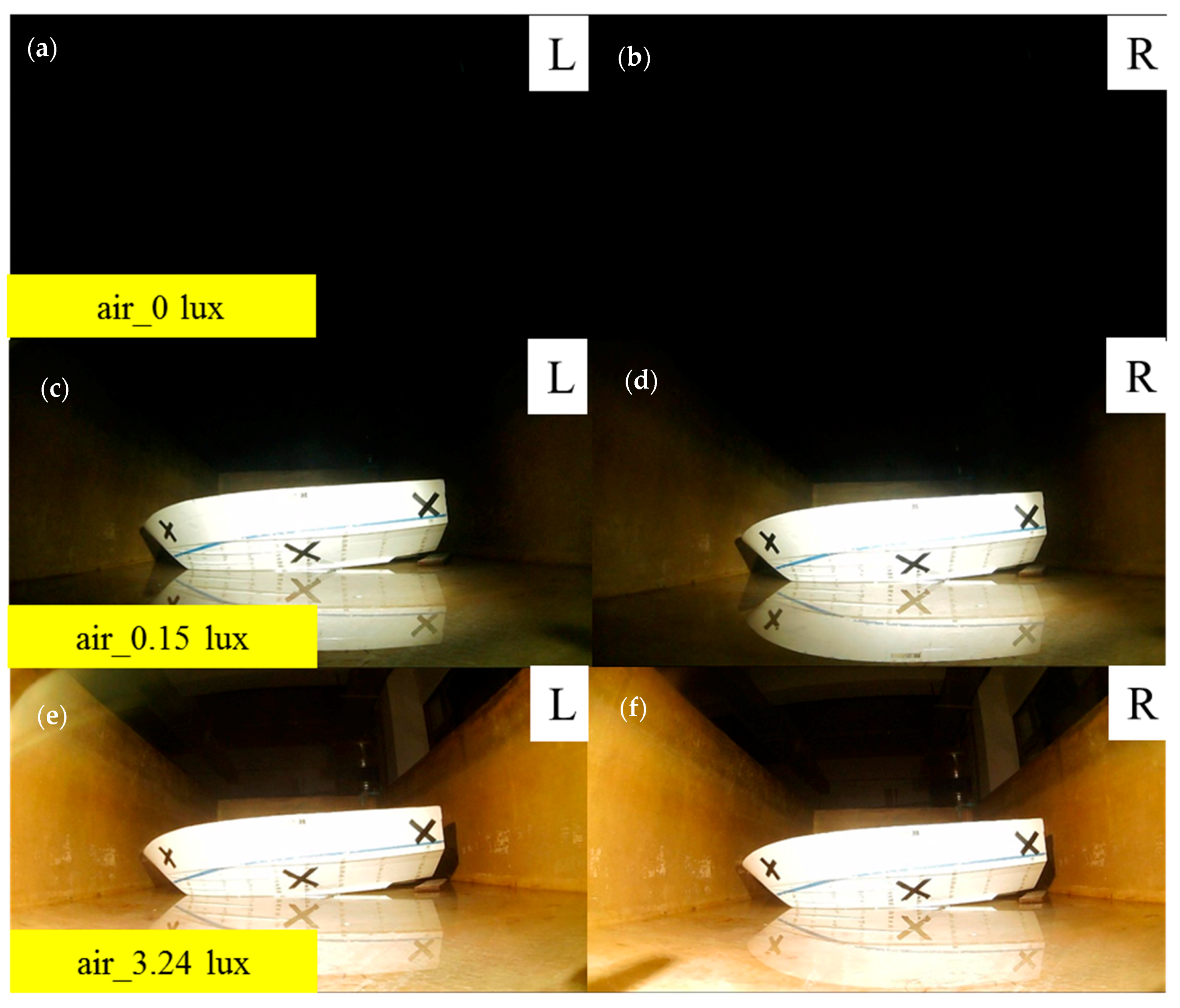
5.1. Laboratory Equipment and Instruments

In order to verify the capability of the image processing module and integrate the post-driver system of the AUV, numerous experiments in the out-of-water and the underwater environments were conducted in the stability water tank (2.8 × 1.15 × 0.75 m), as shown in Figure 13 at Department of Systems and Naval Mechatronic Engineering, National Cheng Kung University (NCKU). The wide-angle camera was used for image recognition, and the dual-lens camera was adopted for distance measurement under various conditions of brightness and turbidity. Subsequently, the captured images from the moving sphere were integrated by the system to acquire the moving speed and the distance for further analysis. In this study, MATLAB 2016a and Visual C++ were integrated with Open Source Computer Vision Library (OpenCV), version 2.4.10. Initiated and developed by Intel Corporation, OpenCV is a free cross-platform computer vision library for the development of real-time image processing and computer vision [39].

This study adopted a wide-angle camera, a dual-lens camera, underwater composite cables (

Table 6. Specification table for underwater composite cables.

Length	20 m
Coax 75 ohm	1 each
Conductor	5/0.25 mm2
Shielded twisted Quad	7/0.2 mm2
Outer jacket	Polyurethane
Diameter	11 ± 0.30 mm
Min. breaking strength	500 kg

), an underwater stabilizer, a power control box, underwater luminaires (

Table 7. Specification table for underwater LED light source.

Pressure Testing	200 bar
Light Power Consumption	200 Watt/Each
Housing	Hard Anodized 6061-T6 Aluminum Alloy
Camera Power Supply	DC 10 V–30 V
Subsea Waterproof Wet Connector	Bulk Head
Operating Temperature (Water)	0~45 °C

), portable lux meter (

Table 8. Specification table for portable lux meter HI97500.

Range	0.001 Klux to 1.999 Klux 0.01 Klux to 19.99 Klux 0.1 Klux to 199.9 Klux
Resolution	0.001 Klux 0.01 Klux 0.1 Klux
Accuracy	±6% of reading ±2% digits
Calibration	Factory calibrated
Light Sensor	Human-eye-response silicon photodiode with 1.5 m coaxial cable

), portable turbidity meter (

Table 9. Specification table for portable turbidity meter HI98703. NTU: Nephelometric Turbidity Units.

Range	0.00 NTU to 9.99 NTU 10.0 NTU to 99.9 NTU 100 NTU to 1000 NTU
Resolution	0.01 NTU from 0.00 NTU to 9.99 NTU 0.1 NTU from 10.0 NTU to 9.99 NTU 1 Klux from 100 NTU to 1000 NTU
Accuracy	±2% of reading plus 0.02 NTU
Repeatability	±1% of reading or 0.02 NTU
Stray Light	<0.02 NTU
Typical EMC Deviation	±0.05 NTU
Light Source	Tungsten filament lamp
Method	Ratio Nephelometric signal scatter light ratio transmitted light Adaptation of the USEPA Method 108.1 and Standard Method 2130B

), and target objects (i.e., an aluminum rod or a ship model). Underwater composite cables are used for connecting the underwater luminaire to the power control box. Underwater stabilizer is made of stainless steel SUS316&PP, this stabilizer has a measurement of 480 × 350 × 195.17 mm. As a fixed amount for luminaires, the stabilizer allows the fixed luminaires to illuminate the underwater environment. Power control box is equipped with multifunctional tools and can provide electricity for the luminaires. The underwater luminaires are the equipment of the underwater light-emitting diode (LED), which is used for simulation of underwater light sources. In order to measure brightness values of the experimental environments, the HI97500-type portable lux meter is implemented. The HI98703-type portable turbidity meter was conducted for the measurement of turbidity in underwater environments. Before the experiment, kaolinite, a type of aluminum-containing silicate mineral that resembles flour with fine particles that do not precipitate easily, was evenly sprinkled into the water to simulate a turbid underwater environment.

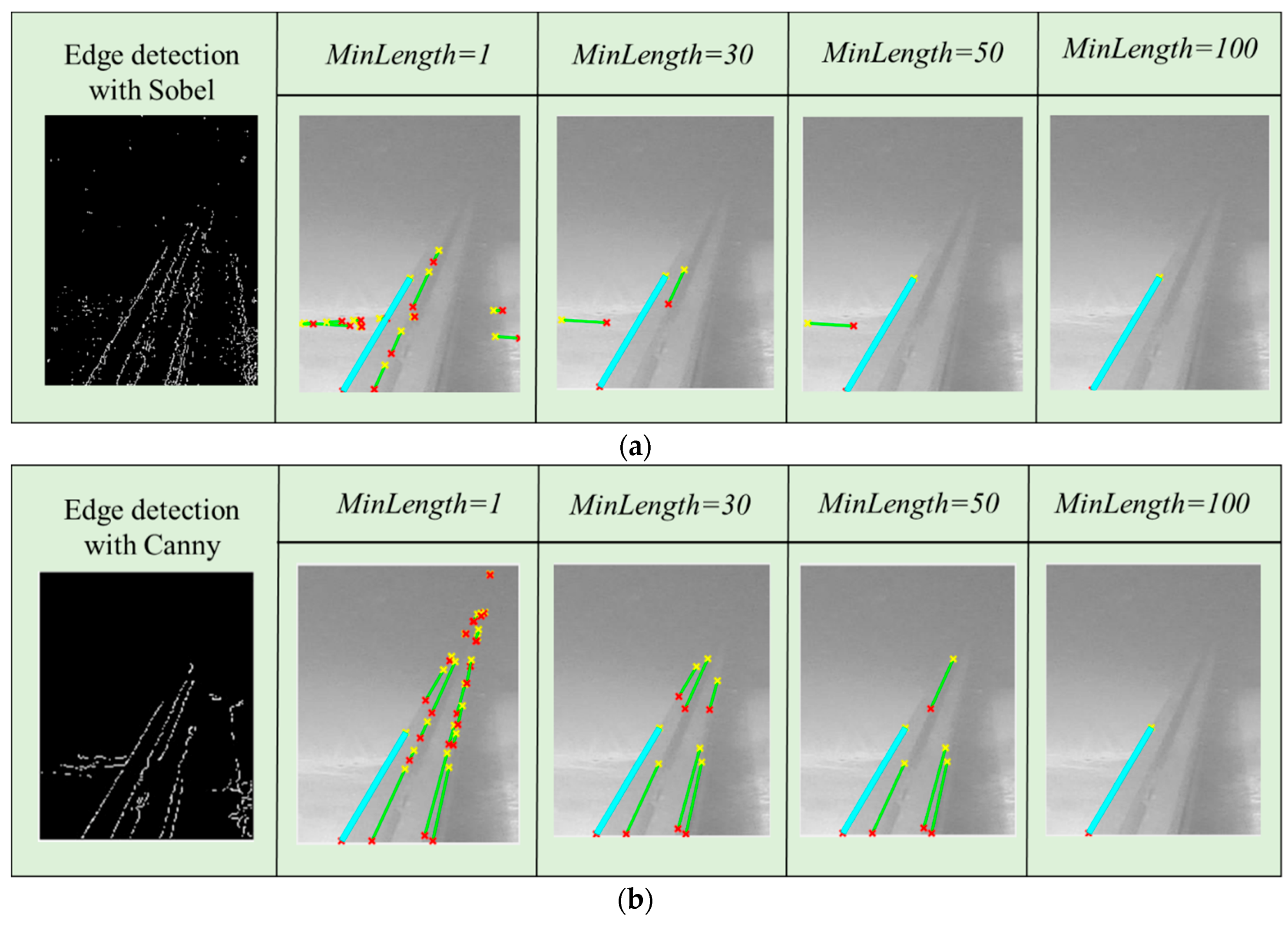
5.2. Hough Transform

An aluminum rod was employed as the main type of target objects in this study because its features resemble the linear features of a pipeline. Images of the aluminum rod were captured by a wide-angle, single-lens camera. Experiments were conducted on the target objects in the out-of-water and the underwater environments as indicated in Figure 14a,b, respectively. The underwater turbidity was 3.31 Nephelometric Turbidity Units (NTU), whereas the illuminance in both environments was 3.24 lux. To improve computing speed, the manually selected ROI was employed to select the target object to focus the computing on the target object while avoiding the extraneous areas (e.g., background) of the image. Such method is particularly efficient in computing high-resolution images. Figure 14c,d show the selected results of the ROI application, which was set to center the target at the center of the image.

For the analysis of line detection, the syntax of the proposed Hough transform is suggested as lines = houghlines(BW, θ, ρ, houghpeaks, FillGap, MinLength), in which consists of a binary image (BW), line rotation angle in radians (θ), distance from the coordinate origin (ρ), the maximum value of the Hough transform space (houghpeaks), distance between two line segments (FillGap), and the minimum length for line illustration (MinLength). Subsequently, the analyzed results acquired from the adjustment of three adjustable parameters, namely houghpeaks, FillGap, and MinLength, would be introduced by comparing Canny edge detector with Sobel edge detector in the out-of-water and underwater environments.

1. Houghpeaks

This parameter identifies the peak value (i.e., number of lines) in Hough transform, which is related to the θ and ρ of polar coordinates for the establishment of Hough Space. Figure 15a,b indicate the analyzed results of the Hough space for the target object (the aluminum rod) in the out-of-water and underwater environments, respectively. The horizontal axis (θ) and the vertical axis (ρ) are presented in the form of polar coordinates, and the number of red squares signifies the number of straight lines detected.

2. FillGap

The parameter FillGap affects the accuracy of the straight-line detection by the proposed Hough transform. A comparison among various FillGap values for the target object measured in the out-of-water environment is presented in Figure 16a. It is evident that when FillGap is 30 or higher, Hough transform algorithm is able to detect both features of the target object and non-features, such as the background. The algorithm can adequately satisfy the purpose of object detection when FillGap is 10 or 20.

Figure 16b shows that multiple straight lines from top left to bottom right are detected when FillGap = 20, 30, 40, 50, and 60. Such results were caused by the irregular size of suspended particles, with short interparticle distance yielding evident features in the image. Furthermore, concentration of suspended particles in the underwater environment has an influence on the detection effect.

In summary, an increase in the FillGap value reduces the accuracy of the line detection algorithm. Parameter adjustment can effectively omit the straight lines that do not belong to the target object, substantially improving the detection accuracy of the proposed Hough transform.

3. MinLength

The parameter MinLength defines the threshold value of line illustration. Any straight line with a parameter that is lower than the threshold value would be omitted during the operation of Hough transform. MinLength can effectively improve line detection accuracy as FillGap does. The following figures are comparison of commonly adopted methods (i.e., Canny and Sobel edge detectors) with various MinLength values. The tests for MinLength were performed with a given value for the parameter FillGap = 10 from the previous experiment.

Figure 17a is a comparison of different MinLength values for a Canny edge detector integrated with Hough transform in the out-of-water environment. The number of lines detected is found to decrease with an increase in MinLength value; this may have been caused by the lack of suspended particles in the out-of-water environment. The detection results basically conform to features of the target object and have no misdetection.

A comparison of different MinLength values for a Sobel edge detector integrated with a Hough transform in the out-of-water environment is illustrated in Figure 17b, in which the detected lines similarly decrease with an increase in MinLength. Without lucid features on the right side of the target object during the operation of the Sobel edge detector, no feature lines were detected in the same region during the calculation of this Hough transform.

Figure 18a presents a comparison of different MinLength values for a Canny edge detector integrated with a Hough transform in the underwater environment. It is revealed that a decrease in lucid lines is accompanied with an increase in MinLength. Since the suspended particles in the water partially cover the edge features of the target object, intermittent lines can be; therefore, observed. Furthermore, the figure on the right side of the target object exhibits the highest number of intermittent lines, which implies that the intensity of suspended particles on the right side was higher than that of the object features.

A comparison of different MinLength values for a Sobel edge detector integrated with a Hough transform in the underwater environment is illustrated in Figure 18b. The analyzed results reveal that intermittent lines are induced by suspended particles in the underwater environment. In addition, the application of this Sobel edge detector scarcely generates any evident features on the right-hand side of the target object.

The results for the two common edge detectors with different MinLength values in the out-of-water and the underwater environments indicate that this integration of a Hough transform and a Canny edge detector has a relatively favorable performance regardless of environment. Since the quality of edge detection determines the accuracy of line detection, this study selected the Canny edge detector as the foundation for a Hough transform for subsequent operations of image recognition.

5.3. Assessment of Stereoscopic Vision

In order to test the capability of stereoscopic vision for the dual-lens camera, a ship model was taken as a target object (Figure 19). In Figure 19, the regions of bow (A), midship (B), and stern (C) of the ship model were defined by different colors. In addition, each region was marked with a black cross sign, which served as a reference for analysis of distance measurement. In this study, the baseline B was set to be 10 cm. Since this study aims to explore the assessment of stereoscopic vision of the ship model in the out-of-water and underwater environments, the ship model was placed at distance d = 1, 1.5, 2, and 2.5 m away from the camera lenses. Subsequently, the left and right CCD cameras each captured an image, after which the distance calculated by the computer was compared with the actual distance to analyze the error rate. Furthermore, this study explored the operation of Harris corner detection before implementing stereoscopic vision matching.

Figure 20a,b shows images captured by left and right lenses under 3.24 lux illuminance and the out-of-water environment, whereas Figure 21a,b presents images captured under 1.1 NTU turbidity and 3.24 lux illuminance in the underwater environment.

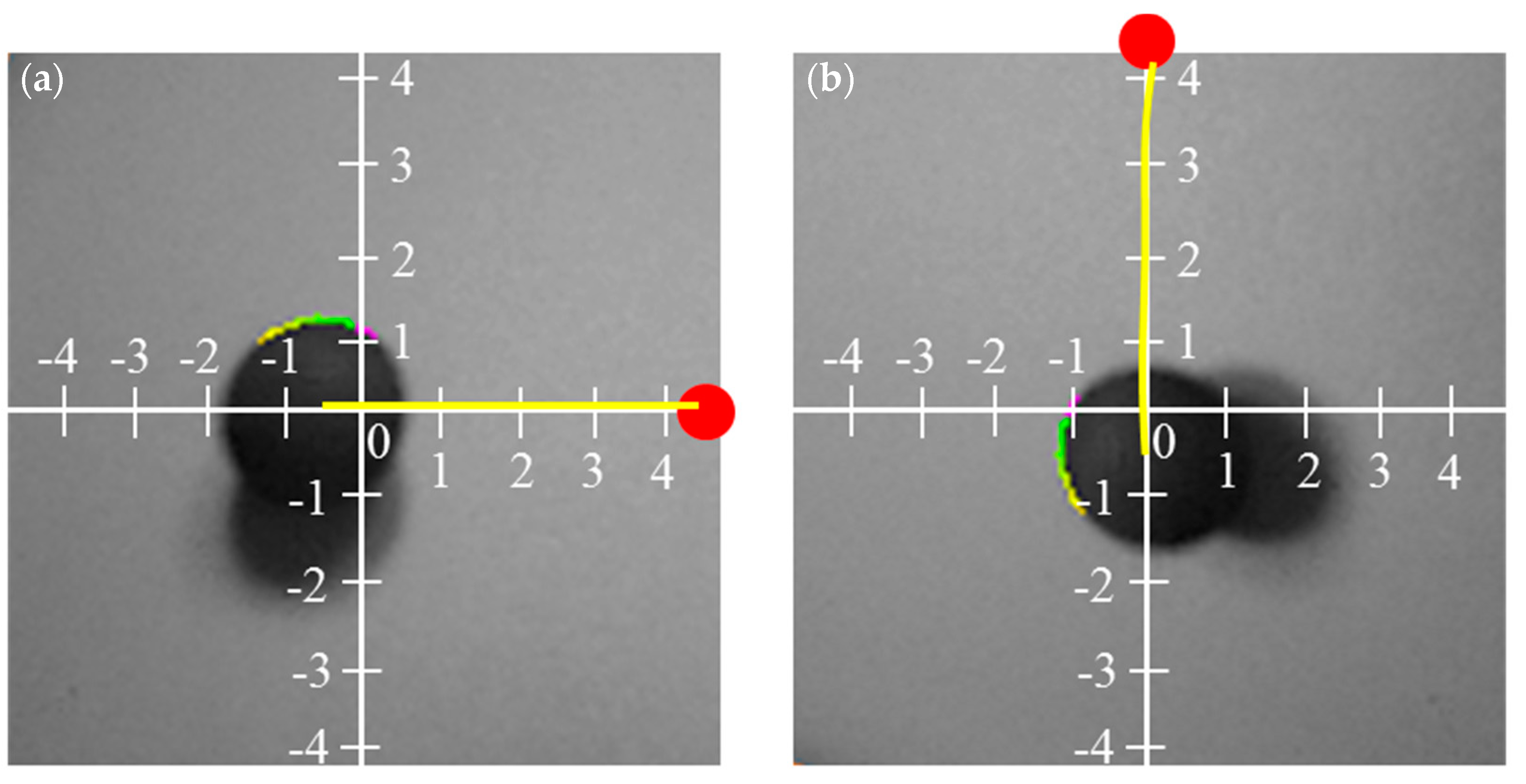
5.3.1. Harris Corner Detector

A Harris corner detector often calculates the corner strength of each pixel in an image, as illustrated in Figure 22a,b. When applied to the ship model in the out-of-water environment, it was exhibited that the Harris corner detector superimposed squares on the image to acquire a corner strength image. Figure 22c,d show partial enlargement of the ship model, in which the detected corners in both images are located at the same feature points on the ship model. Non-local maximum values were used for suppression; the system only retained values higher than the values of neighboring pixels, and then a threshold value was used to filter out corners that exceeded a particular intensity or the value of the fraction of the strongest corner. Another option was to select the strongest top N points.

The results of Harris corner detection in the out-of-water environment are listed in

Table 10. Results of Harris corner detection on target object in the out-of-water environment.

Parameter	Left Image	Right Image
Number of detected corners	7508	7685
Proportion to the total pixels	0.8%	0.8%
Number of selected corners	200	200

. The number of detected corners was the local maximum value in the corner strength image, and occupied approximately 0.8% of the total pixels in the image. The images of partial enlargement indicate that corners were clearly identified for the bow, midship, and stern. In addition, the corners clustered in regions of high contrast and evident patterns; such a phenomenon would result in distortion in practical applications. To achieve even distribution of corners, this study increased the local maximum value through the minimum distance between designated corners.

Harris corner strength after a designated minimum distance in the out-of-water environment is indicated in Figure 23a, where u denotes pixels in the x-direction and v denotes the pixels in the y-direction. According to the corner strength function, the values of feature corners (white) are positive and those of line features (black) are negative. Figure 23b is the Cumulative Distribution Function (CDF) plot for the positive corner strength, where the x-axis represents the corner strength and the y-axis indicates the cumulative probability of feature points. Meanwhile, CDF is a function of corner strength of the image to be processed, of which the value is assumed to be within the range of [0, 1]. CDF can be used for the transformation, which is called histogram equalization or histogram linearization transformation.

On the other hand, Figure 24a,b depicts the corner strength image obtained by applying Harris corner detector to the ship model underwater and superimposing the squares on the image; the corresponding partial enlargement image is illustrated in Figure 24c,d.

Table 11. Results of Harris corner detection performed on target object in the underwater environment.

Parameter	Left Image	Right Image
Number of detected corners	8717	8710
Proportion to the total pixels	0.9%	0.9%
Number of selected corners	200	200

shows the results of Harris corner detection performed on the target object in the underwater environment, in which the number of detected corners was the local maximum value in the corner strength image and accounted for 0.9% of total pixels in the image.

Harris corner strength after a designated minimum distance in the underwater environment is indicated in Figure 25a, where u denotes pixels of the x-direction and v indicates pixels of the y-direction. Because the underwater environment had a relatively low level of contrast, the obtained result was scarce. Figure 25b is the CDF plot for positive Harris corner strength, where the x-axis represents the corner strength and the y-axis indicates the cumulative number of feature points.

Since Harris corner detection is based on the calculation of image gradient, the algorithm is robust to the degree of contrast and feature corners are invariant to rotation. In addition, the detector changes with the scale; if the image is magnified, the gradient in the adjacent corner decreases, which further reduces the strength of surrounding pixels.

5.3.2. Distance Measurement

The target object in Figure 19 was divided into three parts, namely regions A (bow), B (midship), and C (stern). Such evident feature points centered at crosses were selected to calculate the mean values of all obtained distances for regions A, B, and C. According to the actual measurement, the reference values of distances between the camera and regions A, B, and C were 1.1, 1.01, and 1 m, respectively.

Figure 26 shows the images of the target object captured from both sides in the out-of-water environment (labelled as Case 1) with the illuminance parameters of 0, 0.15, and 3.24 lux. Figure 27 illustrates the images of the target object captured from both sides in the underwater environment (labelled as Case 2) with a turbidity of 1.1 NTU and an illuminance parameter of 0, 0.15, and 3.24 lux, respectively.

Table 12. Analysis results obtained from stereoscopic measurement in the underwater environment with turbidity 1.1 NTU (error rate (%) = (|original distance − obtained distance|)/(original distance) × 100%).

Case Type	Region	Original Distance (m)	Measured Distance (m)	Error Rate (%)
Case1_0.15 lux	A	1.10	0.80	27.70
	B	1.01	0.90	10.89
	C	1.00	1.30	30.00
Case1_3.24 lux	A	1.10	1.00	9.09
	B	1.01	0.95	5.94
	C	1.00	1.30	30.00
Case2_0.15 lux	A	1.10	-	-
	B	1.01	-	-
	C	1.00	-	-
Case2_3.24 lux	A	1.10	0.90	18.80
	B	1.01	1.00	0.99
	C	1.00	0.80	20.00

shows the analysis results obtained from stereoscopic image matching, indicating that high turbidity tends to hinder feature matching between images. The empirical results reveal that feature matching fails in instances with an illuminance parameter of 0 lux. In the Case 2 condition with a turbidity of 1.1 NTU and an illuminance of 0.15 lux, the features of target object were obscured by suspended particles, resulting in a matching failure.

In addition, Table 12 indicates that the results obtained from region A (bow) and C (stern) exhibited considerable errors, even demonstrating negative values in two instances (i.e., the measured distance was greater than the original one). Although the configured physical conditions could not be adjusted, it is able to improve calculation accuracy through image processing.

5.3.3. Comparison of Results after Increasing the Contrast

Figure 28a–d present the results of adjusting the contrast in images of the ship model measured in the out-of-water and the underwater environments, respectively. In this study, the contrast of images can be adjusted by using the Harris corner detector that performs feature matching in stereoscopic vision. The core concept of the Harris corner detector is to design a local detection window in the image. When the window makes minimal movements in each direction, the average energy in the window would change. If the variation value of the energy exceeds the designated threshold, the pixel center of the window is the corner point. Special emphasis should be placed on the fact that Case 2 with an illuminance of 0.15 lux in the underwater environment (Figure 28c) was brighter than the image in Figure 27c, accentuating features of the hull.

Table 13. Measured results after the contrast had been increased (error rate (%) = (|original distance − obtained distance|)/(original distance) × 100%).

Case	Region	Original Distance (m)	Obtained Distance (m)	Error Rate (%)
Case1_0.15 lux	A	1.10	1.00	9.09
	B	1.01	1.00	0.99
	C	1.00	0.99	1.00
Case1_3.24 lux	A	1.10	1.00	9.09
	B	1.01	0.96	4.95
	C	1.00	0.95	5.00
Case2_0.15 lux	A	1.10	-	-
	B	1.01	1.01	0.99
	C	1.00	-	-
Case2_3.24 lux	A	1.10	1.09	0.90
	B	1.01	1.00	0.99
	C	1.00	0.92	8.00

shows the measured result after increasing the contrast, whereas

Table 14. Improvement in error rate after the contrast had been increased.

Case	Region	Original Error Rate (%)	Error Rate after Increasing Contrast (%)	Improvement Rate (%)
Case1_0.15 lux	A	27.70	9.09	67.18
	B	10.89	0.99	90.90
	C	30.00	1.00	96.66
Case1_3.24 lux	A	9.09	9.09	0.00
	B	5.94	4.95	16.60
	C	−30.00	5.00	83.33
Case2_0.15 lux	A	-	-	-
	B	-	0.99	-
	C	-	-	-
Case2_3.24 lux	A	18.80	0.90	95.21
	B	0.99	0.99	0.00
	C	20.00	8.00	60.00

indicates the improvement rate between the originally acquired results and those with a relatively high contrast. The results indicate that the error rate is substantially improved after the contrast is increased. Because the characteristics of bow, midship, and stern of the ship model are lucid, the matching effect could be greatly improved to facilitate distance measurement. By increasing the contrast, data in Case 2 under an illuminance of 0.15 lux were perceptible; the obtained data were mainly assembled from the hull section, at which light sources were concentrated. However, features of the target object tend to disappear under any excessive level of contrast.

5.3.4. Computation of Error Rate at Different Distances

The dual-lens camera was conducted at four different distances, namely 1, 1.5, 2, and 2.5 m, to calculate the error rate between the actual distance and the distance obtained from triangulation algorithm. Figure 29a,b present the error rates of the algorithm at different distances in pure water (i.e., 0 NTU) with different luminance levels (i.e., 0.15 and 3.24 lux). The increase in distance caused the target object to occupy less pixels, resulting in a relatively high error rate. The error rate of the camera at different distances in turbid water (i.e., 1.1 NTU) with luminance levels of 0.15 lux and 3.24 lux is illustrated in Figure 29c,d. The results reveal that error rates are affected by both distance and suspended particles.

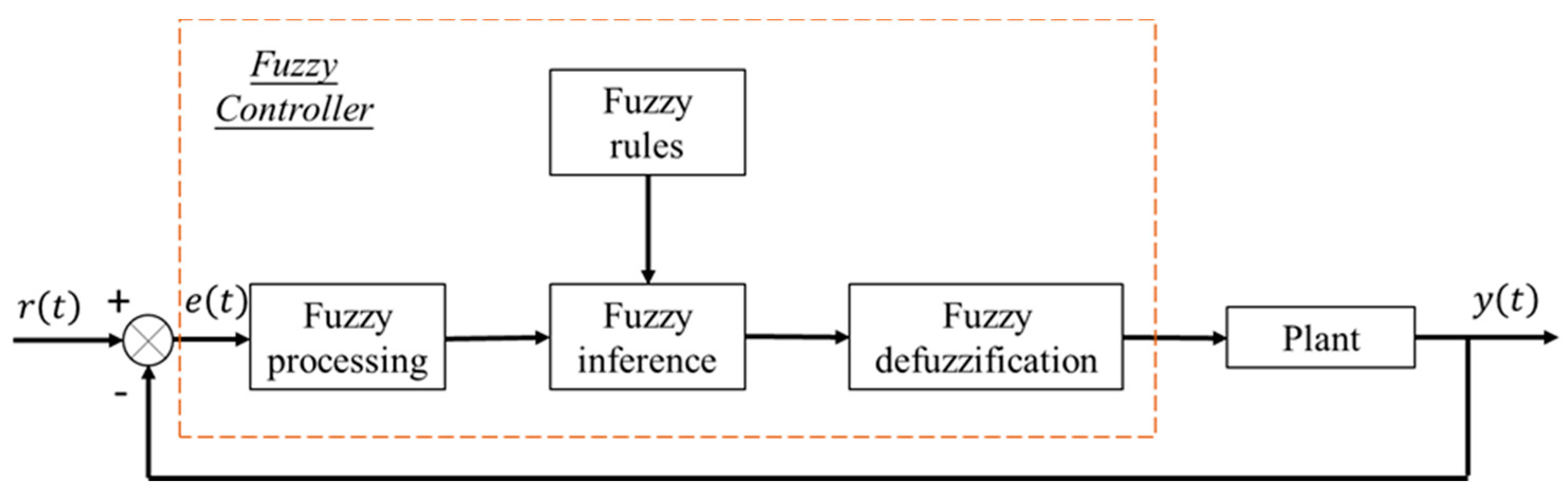
5.4. Integration of Image with Fuzzy Control System

To test the simulation control program, dynamic images of a moving sphere were captured by using the optical flow method (i.e., the movements of the moving sphere from right to left, top to bottom). The sphere is first detected and then tracked through the optical flow method. It is found that the sphere moves from the start point to the end point and its position is divided by a reticle as shown in Figure 30a,b, respectively. Each interval is designated to represent 31 pixel values for convenient and clear marking, which indicates that the sphere occupies 9.09% of the pixels in the entire picture.

Table 15. Condition setting for rudder plane control.

Case	Time (s)	Distance (Pixel)	Speed (Pixel/s)
Case 1	5	155	31
Case 2	10	155	15.5
Case 3	50	155	3.1

indicates the condition settings of three different cases, including the parameters of time, distance, and speed. It is noted that time, distance, and speed describe the movement of the sphere in terms of pixels. More specifically, each case contained vertical and horizontal movements of the sphere and had 1 m of distance from the wide-angle camera.

Figure 31a–f show position-time diagrams on the X–Y plane under different conditions, where the y-axis represents position and the x-axis indicates time. The estimated rotation of vertical and horizontal rudder planes is illustrated in Figure 32a,b, in which the direction ranges from 0° to 180°. In addition, Figure 32c is a schematic diagram of the rotational direction of the propeller.

Since the movement of the sphere is the input condition, parameter settings in Table 15 would be related to the output results of the rudder planes and propeller. For instance, Figure 33a–d indicate the output yaw angle and the corresponding yaw rate of the vertical rudder planes, as well as the output pitch angle and the corresponding pitch rate of the horizontal rudder planes in Case 1. The results of these three cases reveal that the yaw angle of the rudder plane increased with the movement of the sphere; the movement direction of the yaw was also similar to that of the sphere in the image (i.e., right to left and up to down). Therefore, the yaw angle of the rudder plane matched the definition of the rotation direction.

Figure 34a indicates the output of propeller revolution speed based on the distance between the lens and target object, indicating that the revolution speed increased with the distance. The labels in the figure signify the state of occurrence. Figure 34b–d present diagrams at three corresponding states. In state one, the lens starts moving away from the object and the revolution speed starts increasing from 0 rpm; meanwhile, the sphere occupies 86.6% of the total pixels in the image. In state two, the lens continues to stay away from the object and the revolution speed continues to rise; during this state, the sphere occupies 9.52% of the total pixels in the image. In states three, the lens maintains a certain distance away from the object and the revolution speed is gradually reduced to avoid directly reaching 1500 rpm. Meanwhile, the sphere occupies 6.89% of the total pixels in the image.

6. Conclusions

The image processing module (composed of image recognition and stereoscopic matching technology) was integrated with the rudder and propeller of the post-driver system output by a fuzzy controller. This study presents the following conclusions:

• A simulation environment was established for the controlled object (i.e., the steering gear and propeller), and a fuzzy control system was designed particularly for the proposed AUV. With image input, the rotation angle, angular velocity of the rudder plane, and propeller revolution speed can be controlled. In addition, design of the fuzzy attribution function and definition of fuzzy rules can be amended instantly from the simulation interface to reduce system instability and operational uncertainties.
• A Hough transform based on Canny detection was applied to line detection of underwater objects, and the difference in the detection results in the out-of-water and underwater environments was compared. The obtained results indicated that the Hough transform in this study produced notable detection results in both conditions. The adjustment of built-in parameters allowed users to precisely identify the linear features of the object.
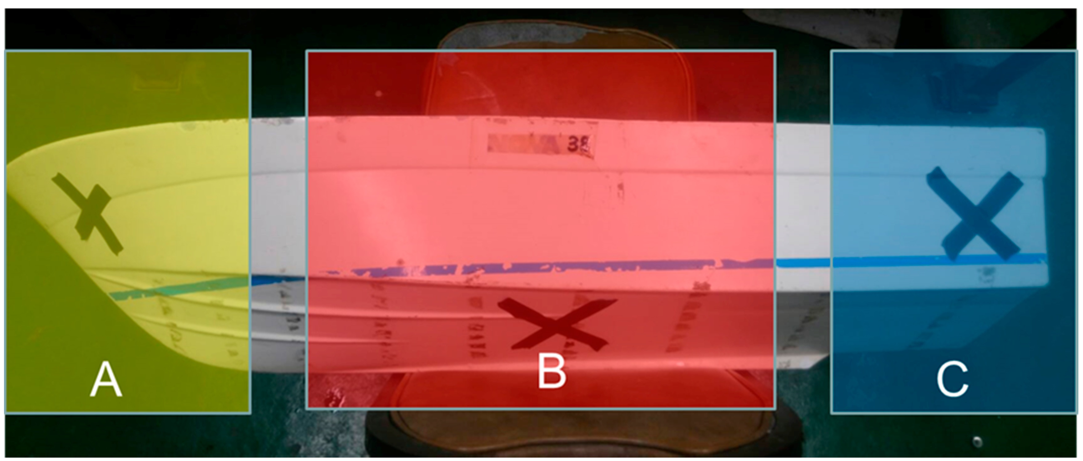
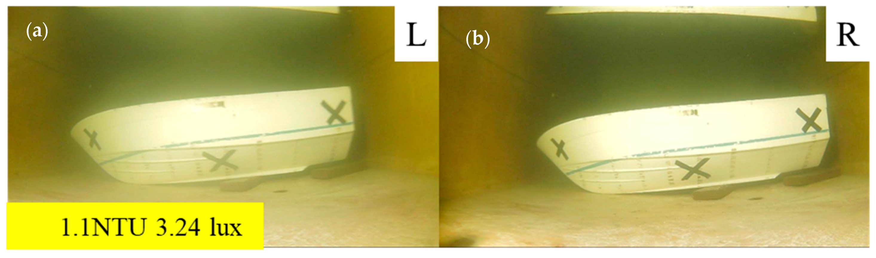
• In terms of distance measurement through stereoscopic vision, it is indicated that graphical features appear distorted unless the contrast is increased in the underwater environment with turbidity. The high contrast ratio results in a substantial increase in the improvement rate, reaching a maximum of 96%, indicating that this image processing method can indeed deliver superior measurement results.
• In future study, the image processing module combined with the fuzzy controller would be applied to the inspection of underwater structures or object tracking of moving objects.

References

1. Bruno, F.; Bianco, G.; Muzzupappa, M.; Barone, S.; Razionale, A. Experimentation of structured light and stereo vision for underwater 3D reconstruction. ISPRS J. Photogramm. Remote Sens. 2011, 66, 508–518. [Google Scholar] [CrossRef]
2. Sáez, J.M.; Escolano, F. Entropy minimization SLAM using stereo vision. In Proceedings of the 2005 IEEE International Conference on Robotics and Automation (ICRA), Barcelona, Spain, 18–22 April 2005; pp. 36–43. [Google Scholar]
3. Lin, Y.-H.; Shou, K.-P.; Huang, L.-J. The initial study of LLS-based binocular stereo-vision system on underwater 3D image reconstruction in the laboratory. J. Mar. Sci. Technol. 2017, 22, 513–532. [Google Scholar] [CrossRef]
4. Cho, Y.; Kim, A. Channel invariant online visibility enhancement for visual SLAM in a turbid environment. J. Field Robot. 2018, 35, 1080–1100. [Google Scholar] [CrossRef]
5. Suresh, S.; Westman, E.; Kaess, M. Through-Water Stereo SLAM With Refraction Correction for AUV Localization. IEEE Robot. Autom. Lett. 2019, 4, 692–699. [Google Scholar] [CrossRef]
6. Teixeira, P.V.; Hover, F.S.; Leonard, J.J.; Kaess, M. Multibeam Data Processing for Underwater Mapping. In Proceedings of the 2018 IEEE/RSJ International Conference on Intelligent Robots and Systems (IROS), Madrid, Spain, 1–5 October 2018; pp. 1877–1884. [Google Scholar]
7. Sáez, J.M.; Hogue, A.; Escolano, F.; Jenkin, M. Underwater 3D SLAM through entropy minimization. In Proceedings of the 2006 IEEE International Conference on Robotics and Automation (ICRA), Orlando, FL, USA, 15–19 May 2006; pp. 3562–3567. [Google Scholar]
8. Sun, B.; Zhu, D.Q.; Yang, S.X. An Optimized Fuzzy Control Algorithm for Three-Dimensional AUV Path Planning. Int. J. Fuzzy Syst. 2018, 20, 597–610. [Google Scholar] [CrossRef]
9. Yu, C.Y.; Xiang, X.B.; Lapierre, L.; Zhang, Q. Nonlinear guidance and fuzzy control for three-dimensional path following of an underactuated autonomous underwater vehicle. Ocean Eng. 2017, 146, 457–467. [Google Scholar] [CrossRef]
10. Lin, Y.H.; Wang, S.M.; Huang, L.C.; Fang, M.C. Applying the stereo-vision detection technique to the development of underwater inspection task with PSO-based dynamic routing algorithm for autonomous underwater vehicles. Ocean Eng. 2017, 139, 127–139. [Google Scholar] [CrossRef]
11. Kularatne, D.; Bhattacharya, S.; Hsieh, M.A. Optimal path planning in time-varying flows using adaptive discretization. IEEE Robot. Autom. Lett. 2018, 3, 458–465. [Google Scholar] [CrossRef]
12. Hermand, E.; Nguyen, T.W.; Hosseinzadeh, M.; Garone, E. Constrained Control of UAVs in Geofencing Applications. In Proceedings of the 2018 26th Mediterranean Conference on Control and Automation (MED), Zadar, Croatia, 19–22 June 2018; pp. 217–222. [Google Scholar]
13. Yao, P.; Zhao, S. Three-Dimensional Path Planning for AUV Based on Interfered Fluid Dynamical System Under Ocean Current (June 2018). IEEE Access 2018, 6, 42904–42916. [Google Scholar] [CrossRef]
14. Foresti, G.L.; Gentili, S.; Zampato, M. Autonomous underwater vehicle guidance by integrating neural networks and geometric reasoning. Int. J. Imaging Syst. Technol. 1999, 10, 385–396. [Google Scholar] [CrossRef]
15. Park, J.-Y.; Jun, B.-h.; Lee, P.-m.; Oh, J. Experiments on vision guided docking of an autonomous underwater vehicle using one camera. Ocean Eng. 2009, 36, 48–61. [Google Scholar] [CrossRef]
16. Wettergreen, D.; Gaskett, C.; Zelinsky, A. Development of a visually-guided autonomous underwater vehicle. In Proceedings of the OCEANS’98 Conference Proceedings, Nice, France, 28 September–1 October 1998; pp. 1200–1204. [Google Scholar]
17. Zhang, T.D.; Wan, L.; Zeng, W.J.; Xu, Y.R. Object detection and tracking method of AUV based on acoustic vision. China Ocean Eng. 2012, 26, 623–636. [Google Scholar] [CrossRef]
18. Armstrong, B.; Wolbrecht, E.; Edwards, D. AUV navigation in the presence of a magnetic disturbance with an extended Kalman filter. In Proceedings of the OCEANS 2010 IEEE-Sydney, Sydney, NSW, Australia, 24–27 May 2010; pp. 1–6. [Google Scholar]
19. Balasuriya, B.; Takai, M.; Lam, W.; Ura, T.; Kuroda, Y. Vision based autonomous underwater vehicle navigation: underwater cable tracking. In Proceedings of the OCEANS’97. MTS/IEEE Conference Proceedings, Halifax, NS, Canada, 6–9 October 1997; pp. 1418–1424. [Google Scholar]
20. Rizzini, D.L.; Kallasi, F.; Aleotti, J.; Oleari, F.; Caselli, S. Integration of a stereo vision system into an autonomous underwater vehicle for pipe manipulation tasks. Comput. Electr. Eng. 2017, 58, 560–571. [Google Scholar] [CrossRef]
21. Balasuriya, A.; Ura, T. Vision-based underwater cable detection and following using AUVs. In Proceedings of the OCEANS’02 MTS/IEEE, Biloxi, MI, USA, 29–31 October 2002; pp. 1582–1587. [Google Scholar]
22. Negahdaripour, S.; Xu, X.; Jin, L. Direct estimation of motion from sea floor images for automatic station-keeping of submersible platforms. IEEE J. Ocean. Eng. 1999, 24, 370–382. [Google Scholar] [CrossRef]
23. Ballard, D.H. Generalizing the Hough transform to detect arbitrary shapes. In Readings in Computer Vision; Elsevier: Amsterdam, The Netherlands, 1987; pp. 714–725. [Google Scholar]
24. Prestero, T.T.J. Verification of a Six-Degree of Freedom Simulation Model for the REMUS Autonomous Underwater Vehicle; Massachusetts Institute of Technology: Cambridge, UK, 2001. [Google Scholar]
25. Litwiller, D. Ccd vs. cmos. Photonics Spectra 2001, 35, 154–158. [Google Scholar]
26. Yamakawa, T. Electronic circuits dedicated to fuzzy logic controller. Sci. Iran. 2011, 18, 528–538. [Google Scholar] [CrossRef] [Green Version]
27. Hu, B.; Tian, H.; Qian, J.; Xie, G.; Mo, L.; Zhang, S. A fuzzy-PID method to improve the depth control of AUV. In Proceedings of the 2013 IEEE International Conference on Mechatronics and Automation (ICMA), Takamatsu, Japan, 4–7 August 2013; pp. 1528–1533. [Google Scholar]
28. Stelzer, R.; Proll, T.; John, R.I. Fuzzy logic control system for autonomous sailboats. In Proceedings of the 2007 IEEE International Fuzzy Systems Conference, London, UK, 23–26 July 2007; pp. 1–6. [Google Scholar]
29. Weber, S. A general concept of fuzzy connectives, negations and implications based on t-norms and t-conorms. Fuzzy Set Syst. 1983, 11, 115–134. [Google Scholar] [CrossRef]
30. Dony, R.; Wesolkowski, S. Edge detection on color images using RGB vector angles. In Proceedings of the 1999 IEEE Canadian Conference on Electrical and Computer Engineering, Edmonton, AB, Canada, 9–12 May 1999; pp. 687–692. [Google Scholar]
31. Gao, W.; Yang, L.; Zhang, X.; Zhou, B.; Ma, C. Based on soft-threshold wavelet de-noising combining with Prewitt operator edge detection algorithm. In Proceedings of the 2010 2nd International Conference on Education Technology and Computer (ICETC), Shanghai, China, 22–24 June 2010; pp. V5-155–V5-162. [Google Scholar]
32. Kanopoulos, N.; Vasanthavada, N.; Baker, R.L. Design of an image edge detection filter using the Sobel operator. IEEE J. Solid-State Circuits 1988, 23, 358–367. [Google Scholar] [CrossRef]
33. Illingworth, J.; Kittler, J. A survey of the Hough transform. Comput. Vis. Graph. Image Process. 1988, 44, 87–116. [Google Scholar] [CrossRef]
34. Kiryati, N.; Eldar, Y.; Bruckstein, A.M. A probabilistic Hough transform. Pattern Recognit. 1991, 24, 303–316. [Google Scholar] [CrossRef]
35. Horn, B.K.; Schunck, B.G. Determining optical flow. Artif. Intell. 1981, 17, 185–203. [Google Scholar] [CrossRef] [Green Version]
36. Bouguet, J.-Y. Camera Calibration Toolbox for Matlab. MRL-Intel Corp. Available online: http://www.vision.caltech.edu/bouguetj/calib_doc/ (accessed on 18 April 2019).
37. Zhang, Z.Y. A flexible new technique for camera calibration. IEEE Trans. Pattern Anal. Mach. Intell. 2000, 22, 1330–1334. [Google Scholar] [CrossRef] [Green Version]
38. Li, J.P.; Yang, Z.W.; Huo, H.; Fang, T. Camera calibration method with checkerboard pattern under complicated illumination. J. Electron. Imaging 2018, 27, 043038. [Google Scholar] [CrossRef]
39. Bradski, G.; Kaehler, A. Learning OpenCV: Computer Vision with the OpenCV Library; O’Reilly Media, Inc.: Sebastopol, CA, USA, 2008. [Google Scholar]
Figure 1. Architecture of the autonomous underwater vehicles (AUV) “Bigeye Barracuda”.
Jmse 07 00107 g001
Figure 2. Block diagram of the fuzzy control theory.
Jmse 07 00107 g002
Figure 3. Fuzzy controller for (a) the vertical rudder plane; (b) the horizontal rudder plane; and (c) the propeller, respectively.
Jmse 07 00107 g003
Figure 4. (a) Input variable 1—membership of yaw angle; (b) input variable 2—membership of yaw rate; (c) output variable 1—membership of the vertical rudder angle; and (d) output variable 2—membership of the vertical rudder angle rate.
Jmse 07 00107 g004
Figure 5. (a) Input variable 1—membership of the pitch angle; (b) input variable 2—membership of the pitch rate; (c) output variable 1—membership of the horizontal plane angle; and (d) output variable 2—membership of the horizontal plane angle rate.
Jmse 07 00107 g005
Figure 6. (a) Input variable—membership of the estimated speed of AUV to reach the target object; (b) output variable—membership of the propeller revolution speed.
Jmse 07 00107 g006
Figure 7. Diagrams of (a) incomplete modeling generated by excessive components; (b) simplified model and coordinate system; and (c) enlargement of post-driver system.
Jmse 07 00107 g007
Figure 8. Flow chart of image processing.
Jmse 07 00107 g008
Figure 9. Edge direction and intensity of a point determined by the gradient.
Jmse 07 00107 g009
Figure 10. Masks of Roberts cross operator (2 × 2), Prewitt operator (3 × 3), and Sobel operator (3 × 3) for horizontal edge detection and vertical edge detection, respectively.
Jmse 07 00107 g010
Figure 11. Flow chart of the probabilistic Hough transform (PHT). (m—each edge point votes for the parameter pairs of all straight lines on which it can lie; k—group the parameter from m; w—the “winning” lines correspond to the largest collinear subsets of edge points in the image).
Jmse 07 00107 g011
Figure 12. Determination of the distance between the cameras and the object in a space through epipolar geometry.
Jmse 07 00107 g012
Figure 13. The experimental set-up and facilities in the stability water tank at Department of Systems and Naval Mechatronic Engineering, NCKU.
Jmse 07 00107 g013
Figure 14. Target object in (a) the out-of-water environment (illuminance of 3.24 lux); and (b) the underwater environment (turbidity of 3.31 NTU and illuminance of 3.24 lux); and images of ROI in (c) the out-of-water environment; and (d) the underwater environment.
Jmse 07 00107 g014
Figure 15. Hough space of the target object in (a) the out-of-water; and (b) the underwater environment, respectively.
Jmse 07 00107 g015
Figure 16. Comparison of various FillGap values of the target object measured in the (a) out-of-water environment; and (b) underwater environment, respectively.
Jmse 07 00107 g016
Figure 17. (a) Canny edge detector; and (b) Sobel edge detector in the out-of-water environment with different MinLength values.
Jmse 07 00107 g017
Figure 18. (a) Canny edge detector; and (b) Sobel edge detector in the underwater environment with different MinLength values.
Jmse 07 00107 g018
Figure 19. Regions of the proposed ship model.
Jmse 07 00107 g019
Figure 20. Images captured by (a) left and (b) right lenses under 3.24 lux illuminance and the out-of-water environment (d = 1 m).
Jmse 07 00107 g020
Figure 21. Images captured by (a) left and (b) right lenses under 1.1 NTU (Nephelometric Turbidity Units) turbidity and 3.24 lux illuminance in the underwater environment (d = 1 m).
Jmse 07 00107 g021
Figure 22. Results of (a) left and (b) right images; and partial enlargement of (c) left and (d) right images from Harris corner detection on the ship model in the out-of-water environment.
Jmse 07 00107 g022
Figure 23. (a) Harris corner strength of the target object; and (b) CDF plot for the positive Harris corner strength in the out-of-water environment (white indicates positive values, whereas black signifies negative values).
Jmse 07 00107 g023
Figure 24. Results of (a) left and (b) right images; and partial enlargement of (c) left and (d) right images from Harris corner detection on the ship model in the underwater environment.
Jmse 07 00107 g024
Figure 25. (a) Harris corner strength of the target object; and (b) CDF plot for the positive Harris corner strength in the underwater environment (white indicates positive values, whereas black signifies negative values).
Jmse 07 00107 g025
Figure 26. Case 1: Images captured from left and right cameras in the out-of-water environment with an illuminance of 0 lux (a,b); 0.15 lux (c,d); and 3.24 lux (e,f).
Jmse 07 00107 g026
Figure 27. Case 2: Images captured from left and right in the underwater environment with a turbidity of 1.1 NTU and an illuminance parameter of 0 lux (a,b); 0.15 lux (c,d); and 3.24 lux (e,f).
Jmse 07 00107 g027
Figure 28. Results of increasing contrast in images of the ship model measured in the out-of-water environment with illuminance of (a) 0.15 lux and (b) 3.24 lux; and in the underwater environment of 1.1 NTU turbidity with illuminance of (c) 0.15 lux and (d) 3.24 lux, respectively.
Jmse 07 00107 g028
Figure 29. Comparison of error rates of (A) bow, (B) midship, and (C) stern measured at four different distances in the condition of (a) 0 NTU and 0.15 lux; (b) 0 NTU and 3.24 lux; (c) 1.1 NTU and 0.15 lux; and (d) 1.1 NTU and 3.24 lux, respectively.
Jmse 07 00107 g029
Figure 30. Markings indicating the movement of the sphere to the end point by (a) horizontal movement and (b) vertical movement by means of the optical flow method.
Jmse 07 00107 g030
Figure 31. Position–time diagrams of X–Y plane: (a) x-axis and (b) y-axis in Case 1; (c) x-axis and (d) y-axis in Case 2; and (e) x-axis and (f) y-axis in Case 3.
Jmse 07 00107 g031
Figure 32. Schematic diagrams of rotation of (a) the vertical rudder plane; (b) the horizontal rudder plane; and (c) the propeller.
Jmse 07 00107 g032
Figure 33. Case 1: (a) Yaw angle and (b) yaw rate of the vertical rudder plane; (c) pitch angle and (d) pitch rate of the horizontal rudder plane.
Jmse 07 00107 g033
Figure 34. Diagrams of (a) output revolution speeds of propeller (rpm); and the corresponding three states: (b) AUV starts moving away from the object at state 1, (c) AUV continues to stay away from the object at state 2; and (d) AUV maintains a certain distance from the object and gradually reduce speed to avoid directly reaching 1500 rpm at state 3 by means of the optical flow method.
Jmse 07 00107 g034