Article

HAMS: A Frequency-Domain Preprocessor for Wave-Structure Interactions—Theory, Development, and Application

Research Institute for Applied Mechanics, Kyushu University, Fukuoka 816-0811, Japan
J. Mar. Sci. Eng. 2019, 7(3), 81; https://doi.org/10.3390/jmse7030081
Submission received: 14 February 2019 / Revised: 10 March 2019 / Accepted: 16 March 2019 / Published: 26 March 2019
(This article belongs to the Special Issue Dynamics of Offshore Structures)

Abstract

:
This paper presents the theoretical background, the numerical implementation, and the applications of a new software that has been developed in recent years for the analysis of wave-structure interactions. The software is developed in the frequency domain, as a preprocessor of computing the wave excitation force, the added mass, and the wave radiation damping, for the input to a time-domain solver via the Fourier cosine and sine transforms. In addition, it can also predict the motion responses of a marine structure with sufficient accuracy, with or without the presence of a mooring system. Unlike other frequency-domain software, such as WAMIT® and Hydrostar®, the present software currently employs the least squares method in association with a partially extended boundary integral equation method to remove the so-called “irregular frequencies”. Calculation of the free-surface Green’s function employs a combination of fast-convergent series expansions in different parametric sub-regions. The solution of the resultant linear algebraic system employs the lower-upper (LU) decomposition method. Symmetry properties can be exploited, and the open multi-processing (OpenMP) parallelization technique can be applied to reduce the computation burden. The accuracy and the efficiency of the developed software are finally confirmed by numerical validations on three benchmark cases of a floating ellipsoid, a truncated circular cylinder and the OC4 DeepCwind semisubmersible floating wind turbine. A free executable version of the software is available to the research communities with a hope of facilitating the advancements in the researches that are relevant to ocean engineering and marine renewable energies.

1. Introduction

Safety and performance are always considered as the first priorities for a marine structure when it is in operation. The sea circumstances can be varied depending on the site location, weather condition, and many other factors. It is preferable for assessments with sufficient reliability to be done before the operation or even before the construction of the marine structure is taken into action. To this end, laboratory experiments are usually performed in advance for model calibrations, wave/load measurements, and system evaluations, etc. However, due to the expensive cost, instead of carrying out the model test for all sea conditions, a reliable numerical tool to assist the assessment in association with a model test in some critical sea conditions are normally employed, which can therefore reduce the overall cost.
So far, to evaluate the overall performance of large marine structures, the boundary integral equation method (BIEM) based on the potential flow theory may still be the first choice over other computational fluid dynamics (CFD) methods based on the N-S equations [1]. This is due to the fact that the viscous term in the N-S equations is not dominant for such a large marine structure when its cross-section diameter D far exceeds 0.15L (in which L is the wavelength) [2]. It should be noted that applying a CFD method is, of course, the best choice for consideration of the accuracy, but the tiny improvement of the accuracy in computation of such a marine structure can hardly compensate the time-consuming computational cost. This problem is especially magnified when the integral performance of the marine structure needs to be quickly evaluated with respect to a batch of input environmental conditions and parameters. In such cases, the computation time of applying a CFD method is incredibly excessive and still not acceptable on up-to-date modern computers.
The BIEM is fundamentally based on the Green’s theorem, by using a free-surface Green’s function that satisfies boundary conditions on the free surface, the seabed, and the far field, the unknowns are reduced to those merely on the immersed body boundary such that the computational burden can be reduced significantly. The remaining computational cost involves two aspects, i.e., the calculation of the free-surface Green’s function and the solution of the resultant linear algebraic system. There are several existing numerical algorithms for fast evaluation of the free-surface Green’s function, e.g., Newman [3,4], Telste and Noblesse [5], and Wu et al. [6] for the deep water, and Newman [3,4], Chen [7,8], and Liu et al. [9,10] for the finite-depth water. Worth noting is that Telste and Noblesse [5] and Liu et al. [10] also released their open-source codes respectively for the deep water and the finite depth water. In respect to the solution of linear equations, there are basically two branches of approaches to choose, i.e., the direct solution methods and the indirect iterative methods. The direct methods, such as the Gauss elimination method, requires a computational effort of 𝒪(N3) operations where N is the dimension of the linear systems. The iterative methods, such as the generalized minimum residual (GMRES) method [11], can reduce the effort to 𝒪(N2) operations but may have a problem of ill preconditions. Meanwhile, taking into consideration the fact that, normally, the radiation-diffraction problem needs to be solved with multiple wave headings for each single wave frequency, the computation effort of using such an iterative method is still high because it needs to successively solve the linear equations for every wave heading.
In addition, another computational issue that should be given attention is the suppression of the so-called “irregular frequencies”. The discrete boundary integral equation is ill-conditioned and not uniquely solvable at these frequencies. The occurrence of such phenomena was firstly discovered by Ref. [12] and later studied by several scholars. There are basically two branches of numerical methods to remove these irregular frequencies: modification of the integral operator or modification of the domain of the integral operator [13,14], and extension of the boundary conditions in Dirichlet or Neumann type [15,16,17]. Although the first branch of methods can theoretically find the unique solutions at all frequencies, they have a critical numerical drawback in calculating the double derivatives of free-surface Green’s function. The second branch of methods requires the solution of a set of completely extended boundary integral equations for which an additional computational effort of evaluating the logarithmic singularity on the free surface is necessary.
This paper presents a new software that solves the above challenging issues. It has been developed for years and tested repeatedly via a series of research and industrial projects. The calculation of free-surface Green’s function employs a combination of series expansions in different parametric subregions with the aid of the epsilon acceleration algorithm, while compromising the accuracy and efficiency of calculations. The solution of the resultant linear algebraic system adopts the lower-upper (LU) decomposition method, which needs to be evaluated only once for the left-hand side matrix over a distribution of wave headings. Removal of the irregular frequencies uses a partially extended boundary integral equation method in association with the least squares method, which reduces the computational effort and avoids evaluation of the logarithmic singularity on the free surface. In addition, symmetry properties are exploited wherever possible for bodies with 1~2 symmetry planes, and the open multi-processing (OpenMP) parallelization technique is applied to the codes in order to reduce the computation time on multi-core machines. The software is therefore named HAMS (Hydrodynamic Analysis of Marine Structures). In the subsequent computations, the computer codes are compiled by Intel® Fortran Compiler 18.0 (Intel® Parallel Studio XE 2018) and Microsoft® Visual Studio 2015.
The remaining part is organized into the following sections: The background theory and the mathematical algorithms of wave-structure interactions are introduced in Section 2. The special techniques of numerical implementation are introduced as separate topics in Section 3. Validation of the software for a simple analytical geometry is given in Section 4.1. Application of the software to marine hydrodynamics of a complex floating structure is carried out in Section 4.2. The conclusions are given in Section 5.

2. Theory and Algorithm

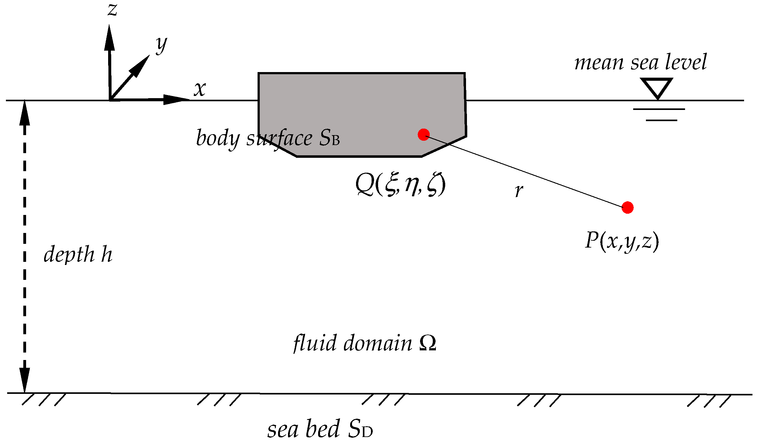
2.1. Governing Equation and Boundary Conditions

The flow is assumed to be inviscid, free of separation or lifting effects, irrorational, and incompressible. In this potential flow framework, the flow can be described by a velocity potential ϕ ( x , y , z ) which can be further decomposed into three parts: the incident wave potential ϕ i ( x , y , z ) , the diffracted wave potential ϕ d ( x , y , z ) , and the radiated wave potential ϕ r ( x , y , z ) :
ϕ = ϕ i + ϕ d + ϕ r .
Mathematically, the above velocity potentials satisfy the Laplace equation in the entire fluid domain
( 2 x 2 + 2 y 2 + 2 z 2 ) ϕ ( x , y , z ) = 0 ,
subjecting to boundary conditions respectively at the free surface, on the body surface, at the sea bottom, and in the far field, as shown in Figure 1, which can be expressed as
ϕ z | z = 0 = v ϕ ϕ n | S B = V n ϕ z | z = h = 0   o r   lim z ( ϕ z ) = 0 lim R [ v R ( ϕ R i v ϕ ) ] = 0 } ,
where v = ω2/g is the wave number in deep water, g is the acceleration of gravity, Vn denotes the normal velocity at a point on the immersed body boundary SB, h is the water depth in case of finite depth water, and R denotes the horizontal distance from the body.
The last boundary condition in Equation (3), also referred to as the Sommerfeld radiation condition, shows that the velocity potential gradually decays with the horizontal distance and eventually vanishes in the far field. It should be noted that the Sommerfeld radiation condition applies only to the scattered potential (including diffracted and radiated wave potentials).
If further using subscripts from 0 to 7 to denote the incident wave potential, the six components of the radiated wave potential, and the diffracted wave potential, then the total velocity potential is expressed as
ϕ = ϕ 0 + ϕ 7 i ω k = 1 6 ξ k ϕ k ,
where the constant ξ k (k = 1,2,…,6) denotes the complex amplitudes of the body oscillation motion in its six rigid-body degrees of freedom, and ϕ k   ( k = 1 , 2 , , 6 ) denotes the corresponding unit-amplitude radiation potentials. In the framework of the Airy wave theory, the incident wave potential ϕ 0 is defined by
ϕ 0 = i g A ω e v z e i v ( x c o s β + y s i n β )
for infinite depth water and
ϕ 0 = i g A ω cosh k ( z + h ) cosh k h e i k ( x c o s β + y s i n β )
for finite depth water, where β is the angle between the direction of propagation of the incident wave and the positive x-axis, and k is the real positive root of the water wave dispersion equation.

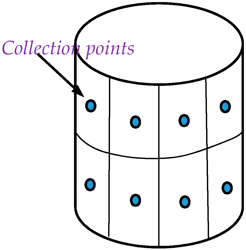
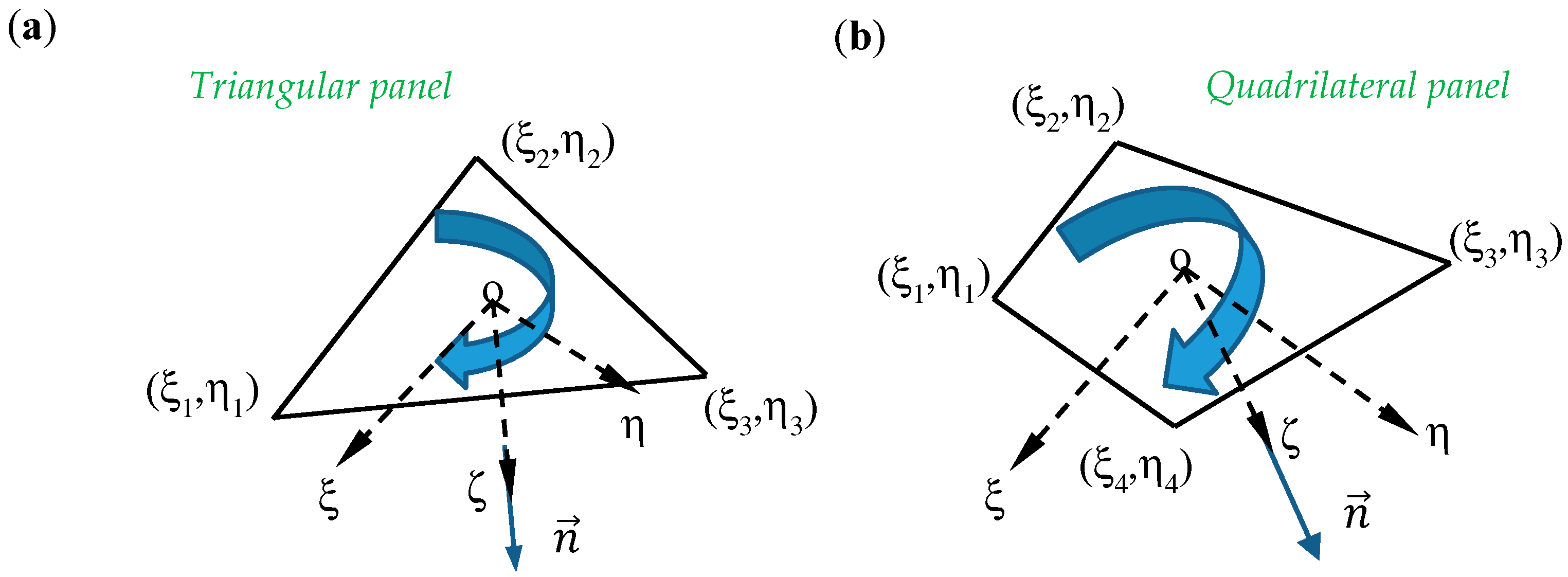
2.2. Mixed Source/Dipole Formulation and Discretization of the Integral Equations

By applying Green’s theorem, the radiated and diffracted wave velocity potentials on the immersed body surface SB are solved by the mixed source/dipole boundary integral equations. The integral equation satisfied by the radiation velocity potential on the body boundary takes the form of
2 π ϕ k ( x ) + S B ϕ k ( x ) G ( ξ ; x ) n ξ d S ξ = S B V n , k ( ξ ) G ( ξ ; x ) d S ξ ,   ( k = 1 , 2 , , 7 ) ,
where ξ denotes the source point, x denotes the field point, and V n , k denotes the kth component of the body surface boundary condition.
The boundary surfaces are discretized into a set of quadrilateral or triangular plane panels to approximate the exact geometry. The vertices of each panel are numbered in the counter-clockwise direction when the panel is viewed from the fluid domain. The radiation and diffraction velocity potentials are also represented by piecewise constant functions over each panel. By applying such a “collection method”, as shown in Figure 2, the boundary integral equations (Equation (7)) are discretized into
2 π ϕ k ( x i ) + j = 1 N p D i j ϕ k ( x j ) = j = 1 N p S i j V n , k ( x j ) ,   ( i = 1 , 2 , , N p ;   k = 1 , 2 , , 7 ) ,
where N p is the number of panels. The integrations of sources and dipoles over each panel are represented by
S i j = S B , j G ( ξ ; x i ) d S ξ ,
D i j = S B , j G ( ξ ; x i ) n ξ d S ξ ,
where S B , j denotes the jth panel surface.

2.3. Evaluation of Green’s Function and Self-Influences

In the boundary integral equations (Equation (7)), numerical evaluation of free-surface Green’s function G(x; ξ) becomes the most essential task due to its highly complex nature. It is not trivial, because of the three sticking points that need to be overcome: the singularity in the denominator of the integrand, the oscillation nature of the Bessel function, and the integration range from 0 to infinity. The Green function G(x; ξ), or source potential, is usually defined as the velocity potential at the field point (x, y, z) due to a point source of strength (−4π) located at the source point (ξ, η, ζ). The Green function is defined by
G = 1 r + 1 r 1 + 2 v π 0 e μ ( z + ζ ) μ v J 0 ( μ R ) d μ
for infinite water depth and
G = 1 r + 1 r 2 + 2 0 ( μ + v ) cos h μ ( z + h ) cos h μ ( ζ + h ) μ sin h μ h v cos h μ h e μ h J 0 ( μ R ) d μ
for finite water depth, where the path of the contour integral passes below the pole at μ = v in Equation (11) and at μ = k in Equation (12). J0(x) is the Bessel function of zero order. r is the distance between the source point and the field point, r 1 denotes the distance between the field point and the image of the source point with respect to the mean free-surface, and r 2 denotes the distance between the field point and the image of source point with respect to the sea bottom:
r = { R 2 + ( z ζ ) 2 } 1 / 2 ,
r 1 = { R 2 + ( z + ζ ) 2 } 1 / 2 ,
r 2 = { R 2 + ( z + ζ + 2 h ) 2 } 1 / 2 .
Currently, the algorithm in Ref. [18] has been applied to evaluate Equation (11), and a newly developed special algorithm [10] has been applied to evaluate Equation (12).
Due to the strong singularity of the Rankine source r−1, the integration of it over each panel is evaluated separately using an analytical algorithm [19]. To this end, as shown in Figure 3, a local coordinate system, o ξ η ζ , needs to be established for each panel by taking the ξ o η plane at the panel surface and the ζ axis along its normal direction. Assuming the field point in the new local system to be ( x , y , z ) , and the coordinates of vertices of each panel in a counter-clockwise direction to be ( ξ n , η n , ζ n ) , where n = 1 , 2 , , N v , N v is the number of vertices on each panel, the formulation for calculating the Rankine part integration can be derived as follows:
i j = S B , j n ξ ( 1 r ) d S ξ = n = 1 N v [ a r c t a n ( c n , n + 1 Q n P n z R n ) a r c t a n ( c n , n + 1 Q n + 1 P n + 1 z R n + 1 ) ]
K i j = S B , j 1 r d S ξ = n = 1 N v [ ( x ξ n ) ( η n + 1 η n ) ( y η n ) ( ξ n + 1 ξ n ) L n , n + 1 ] l o g ( R n + R n + 1 + L n , n + 1 R n + R n + 1 L n , n + 1 ) z i j
where
P n = ( x ξ n ) ( y η n ) ,
Q n = { ( x ξ n ) 2 + z 2 } 1 / 2 ,
R n = { ( y η n ) 2 + Q n 2 } 1 / 2 ,
c n , n + 1 = ( η n + 1 η n ) / ( ξ n + 1 ξ n ) ,
L n , n + 1 = { ( ξ n + 1 ξ n ) 2 + ( η n + 1 η n ) 2 } 1 / 2 .
By taking advantage of the above formulation, the singularities encountered in the boundary integral equations can be evaluated successfully without difficulties.

2.4. Solution of the Linear Algebraic System

In order to solve the linear algebraic system Equation (8), a direct solver such as Gauss elimination will commonly be adopted. These direct solvers are generally robust but require O ( N 3 ) computations (N denotes matrix size). For a large-scale computation of complex three-dimensional offshore structures, a direct inversion or inefficient iteration of such a large, dense system of linear equations with O ( N 4 ) unknowns for a set of wave frequencies seems prohibitively time consuming even with modern computers. On the other hand, although some iterative methods, such as the GMRES method [11], can reduce the effort to O ( N 2 ) operations; however, these kinds of iterative methods can easily have a problem of ill preconditions. In addition, considering the usual cases when the radiation-diffraction problem needs to be solved with multiple wave headings for each single wave frequency, the computation effort of using either a direct method or an iterative method is still not acceptable because it needs to successively solve the linear equations for every wave heading. For this reason, the LU decomposition is adopted in the solver, since it only needs to decompose the left-hand side matrix once for each wave frequency. This decomposition can be applied to calculate the wave forces for a distribution of wave headings via a forward and backward substitution for triangular matrices (L and U), which can be solved directly without using the Gaussian elimination process.

3. Numerical Techniques in Specialized Topics

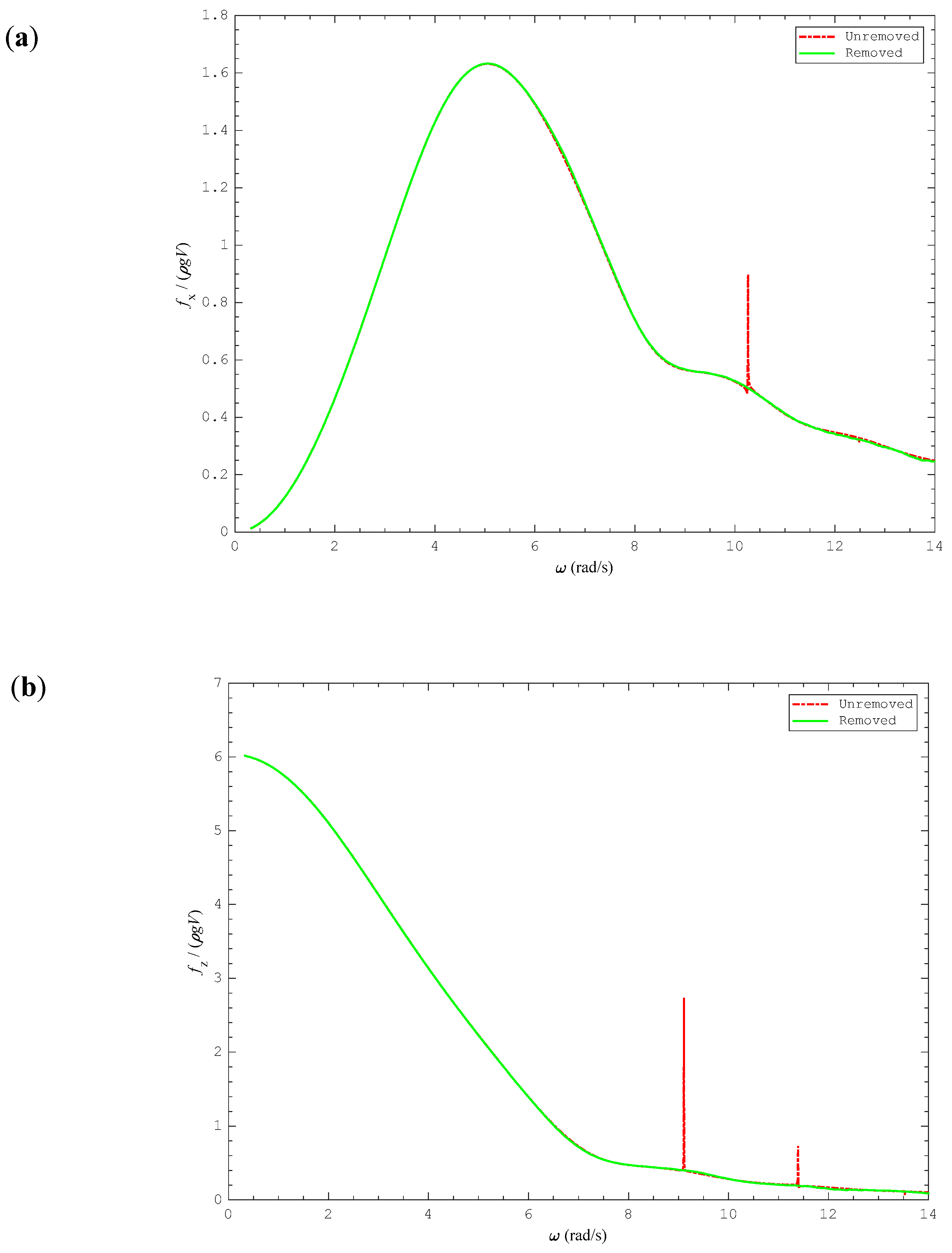
3.1. Removal of Irregular Frequencies

Numerical solutions of Equation (7) possess substantial errors in the neighborhood of the so-called “irregular frequencies”. This phenomenon is caused by the water-plane section of the members of floating bodies that intersects the free water surface. The irregular frequencies actually coincide with the eigenfrequencies of the corresponding sloshing modes of the interior tank (assuming flow filling inside the tank).
In order to suppress these frequencies, a kind of partially extended boundary integral equation can be developed, which assumes that the potentials on the interior water plane are zero. This method originates from Ref. [20]. Therefore, by applying Green’s theorem in the interior domain of the floating body, an additional boundary integral equation is introduced in a combined application with Equation (7):
S B ϕ k ( x ) G ( ξ ; x ) n ξ d S ξ = S B V n , k ( ξ ) G ( ξ ; x ) d S ξ ,   ( k = 1 , 2 , , 7 , x S WP , ξ S B ) ,
where S WP denotes the interior water-plane area. By discretizing S WP into M elements, a set of over-determined linear algebraic equations can be obtained as follows:
[ A ] ( M + N ) × N { ϕ } N = { B } ( M + N ) × N .
Equation (24) can be solved by the least squares method. Defining the square error function as
E = m = 1 M + N [ n = 1 N A m n ϕ k ( x n ) B k ( x m ) ] 2 ,
and optimizing Equation (25) to be of minimum square error
E ϕ k ( x n ) = 0 ,   ( n = 1 , 2 , , N ) ,
a new set of equations which are free of irregular frequencies can be developed instead of Equation (8):
n = 1 N { m = 1 M + N A m n A m p } ϕ k ( x n ) = m = 1 M + N A m p B k ( x m ) ,   ( p = 1 , 2 , , N ) ,
which is not over-determined and thus can be solved directly.
The present method for removing irregular frequencies avoids evaluation of the logarithmic singularity [21] of free-surface Green’s function occurring in the limiting case when that panel is on the free surface. This can be viewed as an advantage which makes the programming simpler. Besides, since the size of the left-hand side matrix in Equation (27) is N × N, which is less than that of (M + N) × (M + N) in Lee’s method [21], the additional numerical work on resolving a larger linear algebraic system can be avoided.

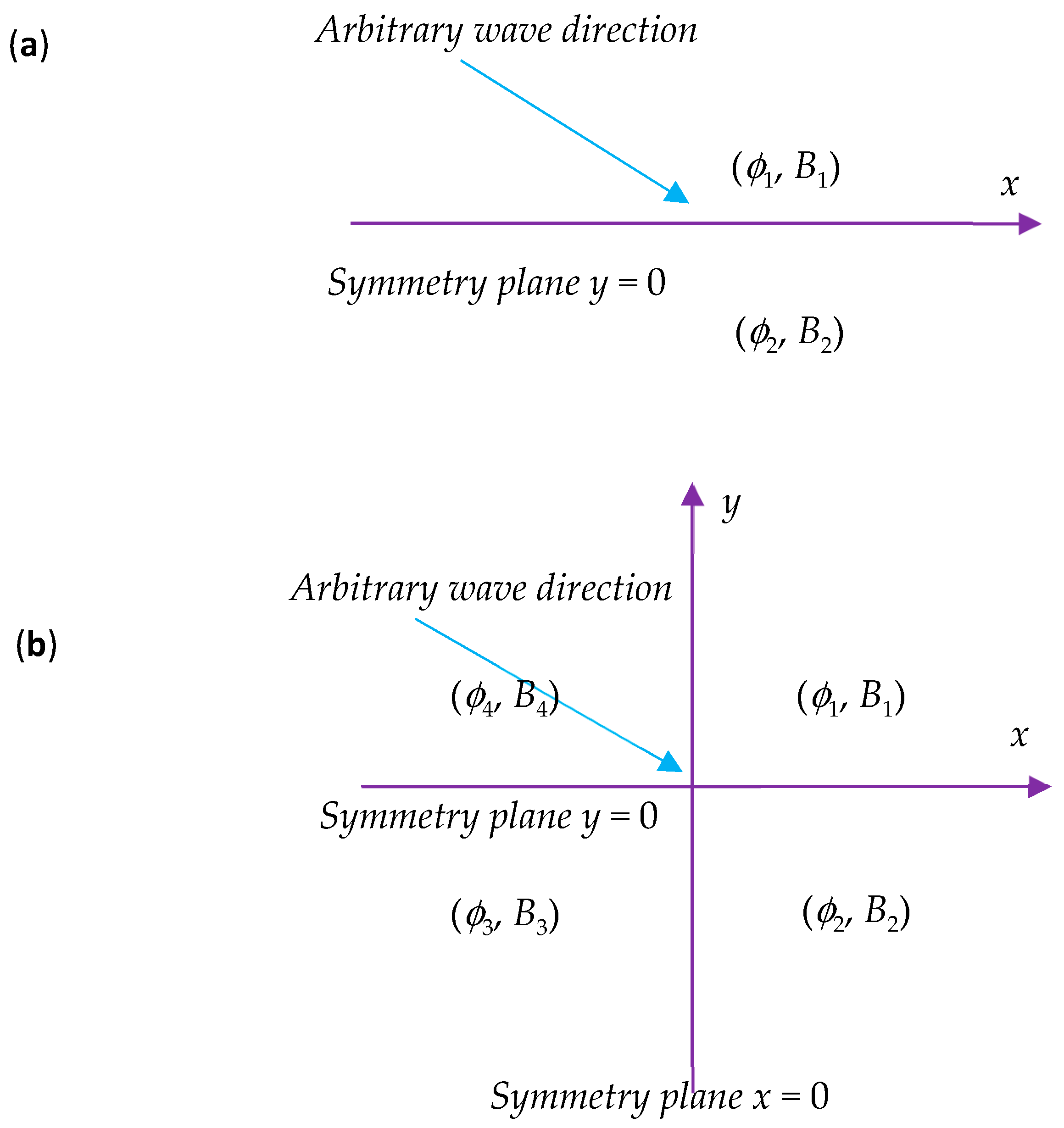
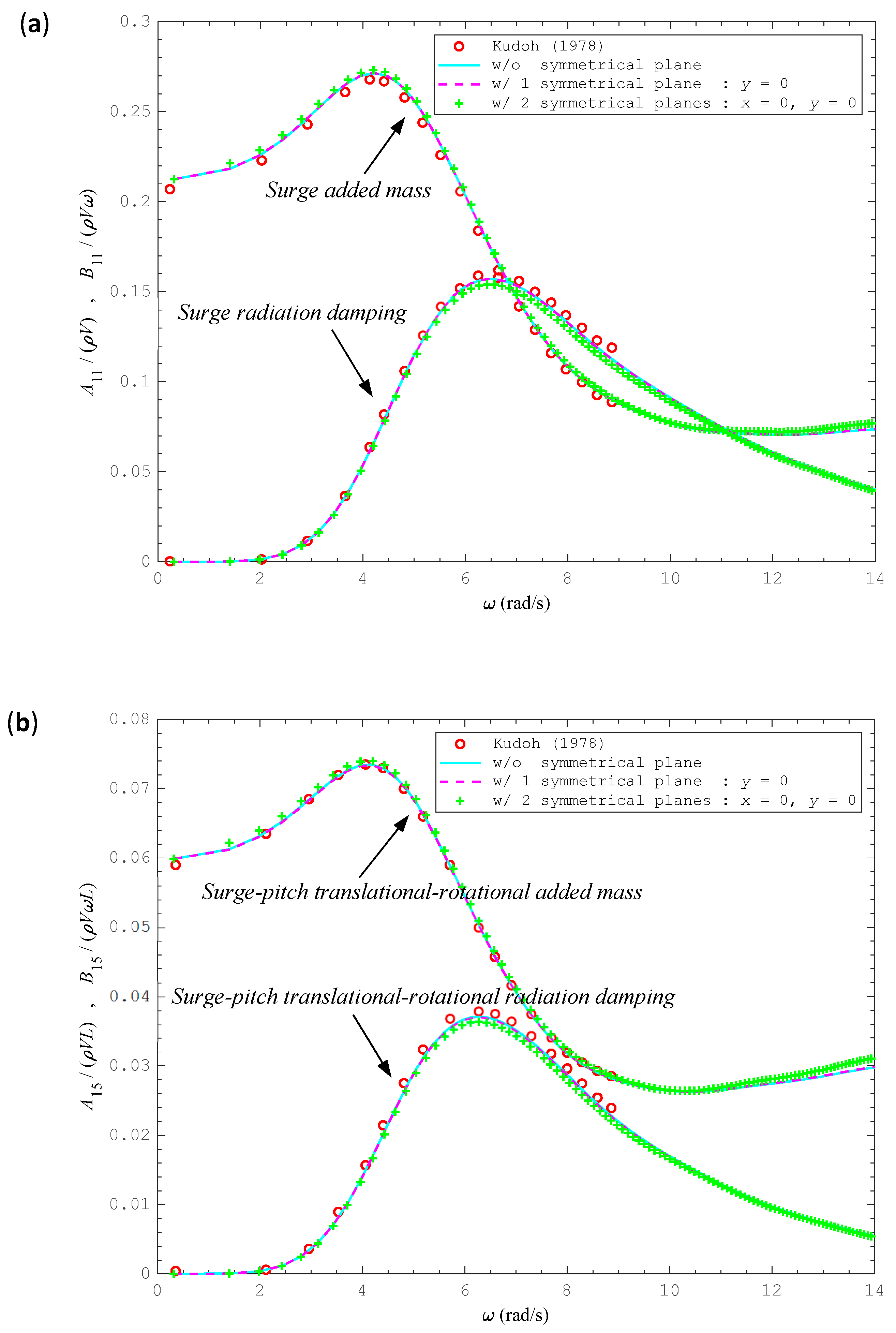
3.2. Exploitation of Symmetrical Properties

The efficiency of the solution method for the boundary integral equations may dramatically increase for bodies having one or two planes of symmetry, because the computation time and storage are saved. In the analysis below, symmetry is therefore exploited wherever possible [22,23].
The discretized form of the boundary integral equation, i.e., Equation (8) or Equation (27), can be expressed in the following matrix form:
[ A ] { ϕ } = { B } .
It is possible to partition the matrix A, the vector ϕ , and B according to the number of symmetry planes. For the body having two planes of symmetry, the following partitions can be found
[ A ] = [ A 11 A 12 A 13 A 14 A 21 A 22 A 23 A 24 A 31 A 32 A 33 A 34 A 41 A 42 A 43 A 44 ] ,
{ ϕ } = { ϕ 1 ϕ 2 ϕ 3 ϕ 4 } T ,
{ B } = { B 1 B 2 B 3 B 4 } T ,
where A 11 is the submatrix of coefficients associated with the discretization of boundary region 1, while A 12 , A 13 , and A 14 are corresponding submatrices arising from the coupling between the boundaries 1 and 2, 3, and 4, respectively. ϕ 1 , ϕ 2 , ϕ 3 , and ϕ 4 are the vectors of components of the velocity potential corresponding to elements in boundaries 1, 2, 3 and 4 respectively. Similarly, B 1 , B 2 , B 3 , and B 4 are the right-hand side vectors associated with boundaries 1, 2, 3, and 4 respectively. Additionally, the following relations are necessary to be employed in the calculation:
A 11 = A 12 = A 13 = A 14 A 21 = A 22 = A 23 = A 24 A 31 = A 32 = A 33 = A 34 A 41 = A 42 = A 43 = A 44 } .
An orthogonal transformation matrix [ R ] can be introduced to reduce the size of the linear system such that
[ A ^ ] = 1 N s [ R ] [ A ] [ R ] ,
{ ϕ ^ } = [ R ] { ϕ } ,
{ B ^ } = [ R ] { B } ,
where N s denotes the number of symmetry planes. This transformation enables the linear system resulting into a simplified diagonal form:
[ A ^ ( 1 ) 0 0 0 0 A ^ ( 2 ) 0 0 0 0 A ^ ( 3 ) 0 0 0 0 A ^ ( 4 ) ] { ϕ ^ ( 1 ) ϕ ^ ( 2 ) ϕ ^ ( 3 ) ϕ ^ ( 4 ) } = { B ^ ( 1 ) B ^ ( 2 ) B ^ ( 3 ) B ^ ( 4 ) } ,
which leads to
{ ϕ ^ ( k ) } = [ A ^ ( k ) ] 1 { B ^ ( k ) } , where   k = 1 , 2 , , N s
Combining Equation (37) with Equations (33)–(35), the solution of { ϕ } can be finally obtained with sufficient accuracy. The partition process is also illustrated in Figure 4.

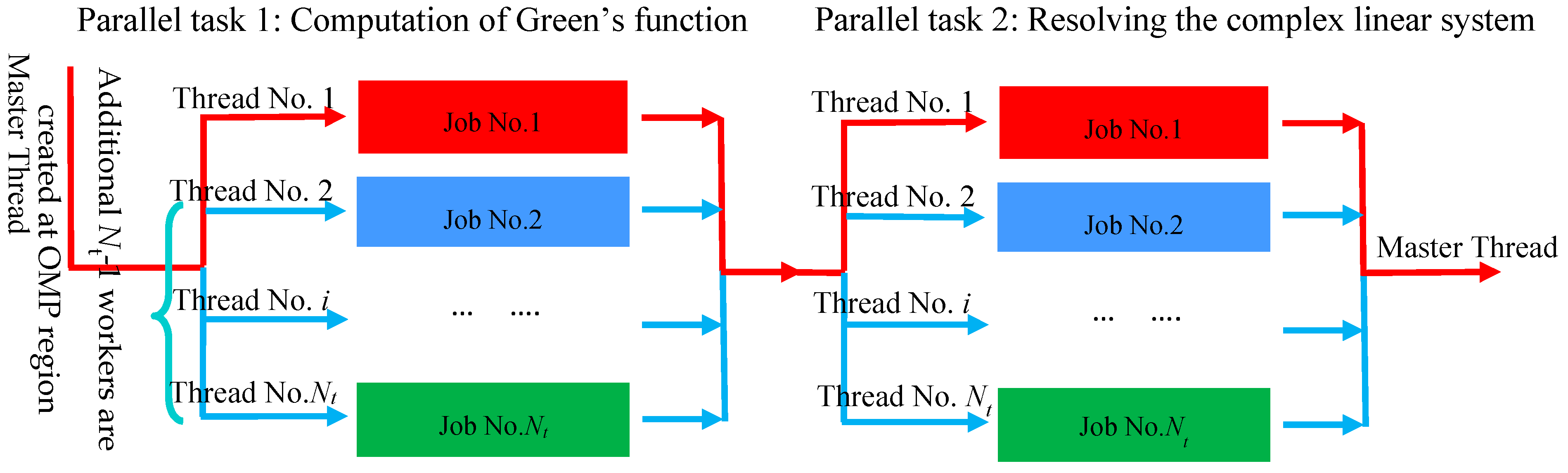
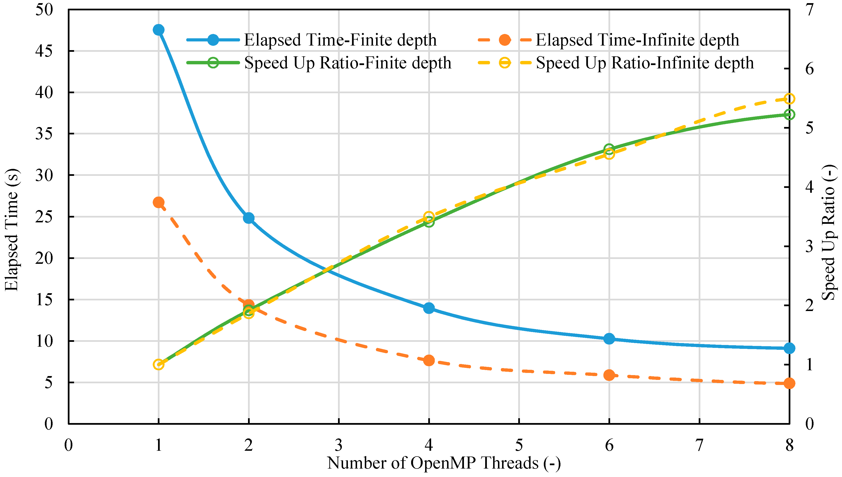
3.3. OpenMP Parallelization on Multi-core Machines

The problems to be solved are often of a very large size such that resolving the resultant linear systems requires huge computational resources. Nowadays, with the facility of a fast multi-core computer, it is natural to maximize the advantages of the current hardware technology in our computations. A large portion of programs that people write and run daily are serial programs, especially in the marine hydrodynamic field as far as the author knows. The serial program runs on a single computer, typically on a single processor, which might be considered as a waste of computational resources. For this reason, it is better to code the program in parallel mode, which will enable the program to run simultaneously on multiple processors. Taking into consideration that in a typical case, the number of panels involved in the hydrodynamic computation is usually below 10~30 thousand, and that off-the-shelf computation machines contain multiple processors, the OpenMP technique is evidently the most suitable for the work in the present study.
The OpenMP standard for Fortran was first released in 1997. It is a standard application programming interface (API) for writing shared memory parallel applications in C, C++, and Fortran. OpenMP has the advantage of being very easy to implement on currently existing serial codes and allowing incremental parallelization [24]. It also has the advantage of being widely used, highly portable, and ideally suited to multi-core architectures, which are becoming increasingly popular in up-to-date desktop computers.
As shown in Figure 5, an OpenMP program usually begins with a single process called the master thread. The master thread executes sequentially until a parallel region is encountered. At this point, the master thread “forks” into a number of parallel worker threads, each of which shares a portion of the computation task. The instructions in the parallel region are then executed by the team of worker threads. At the end of the parallel region, the threads synchronize and join to become the single master thread again [24].
Based on the Amdahl’s Law, if we suppose p (0 < p < 1) part of the program can be run in parallel, on an Nt-thread computational platform, the speed-up ratio R s can be expressed as
R s = 1 ( 1 p ) + p N t .
This means that the maximum speed-up ratio will be Nt by letting p approach unity. However, since the sequential part of work in typical cases is not always zero, this maximum speed-up ratio will generally not be easily reached. Nevertheless, enhancing the serial code to minimize the sequential work is quite necessary to improve the computational speed.

4. Applications to Waves–Structure Interactions

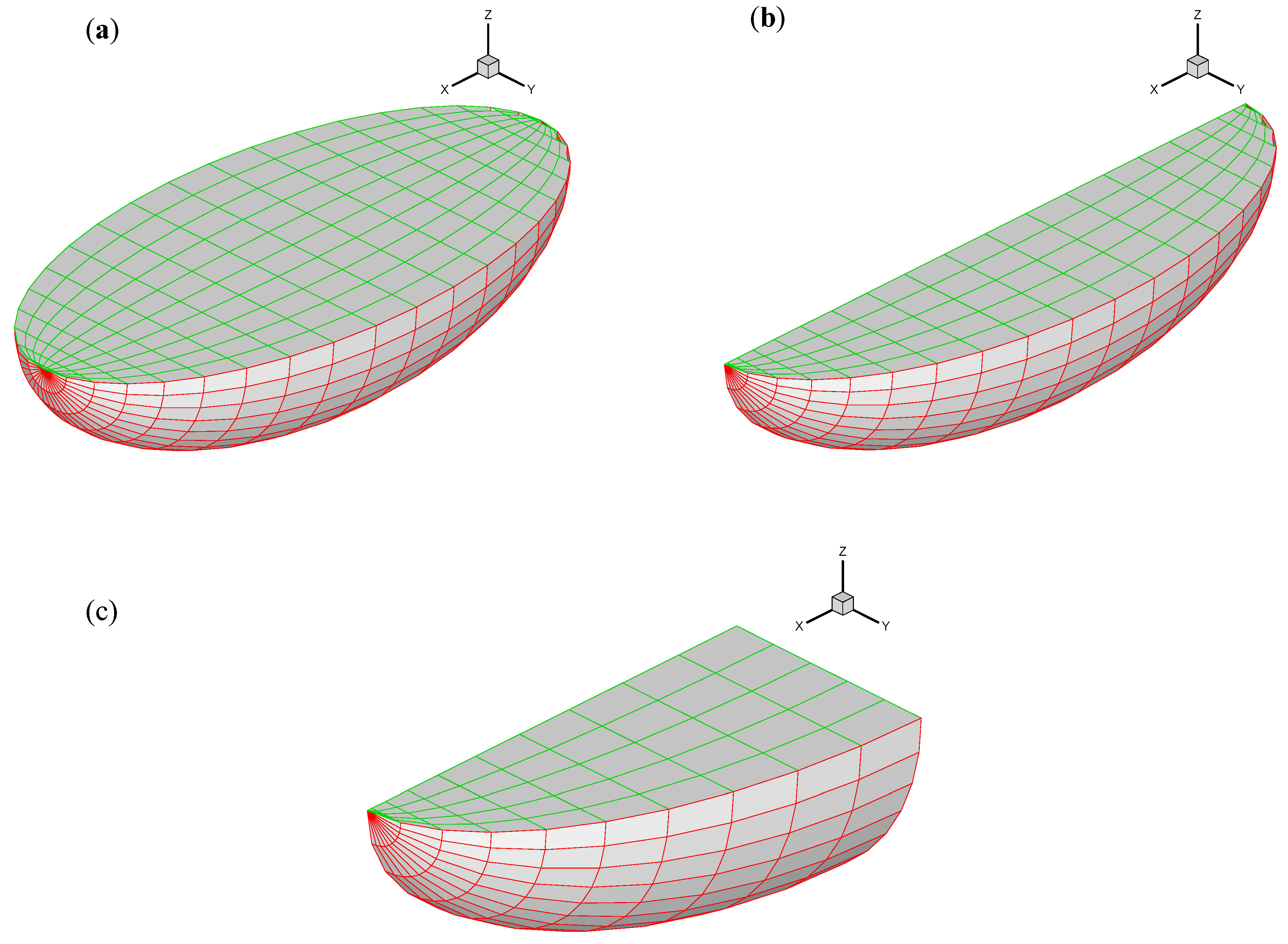
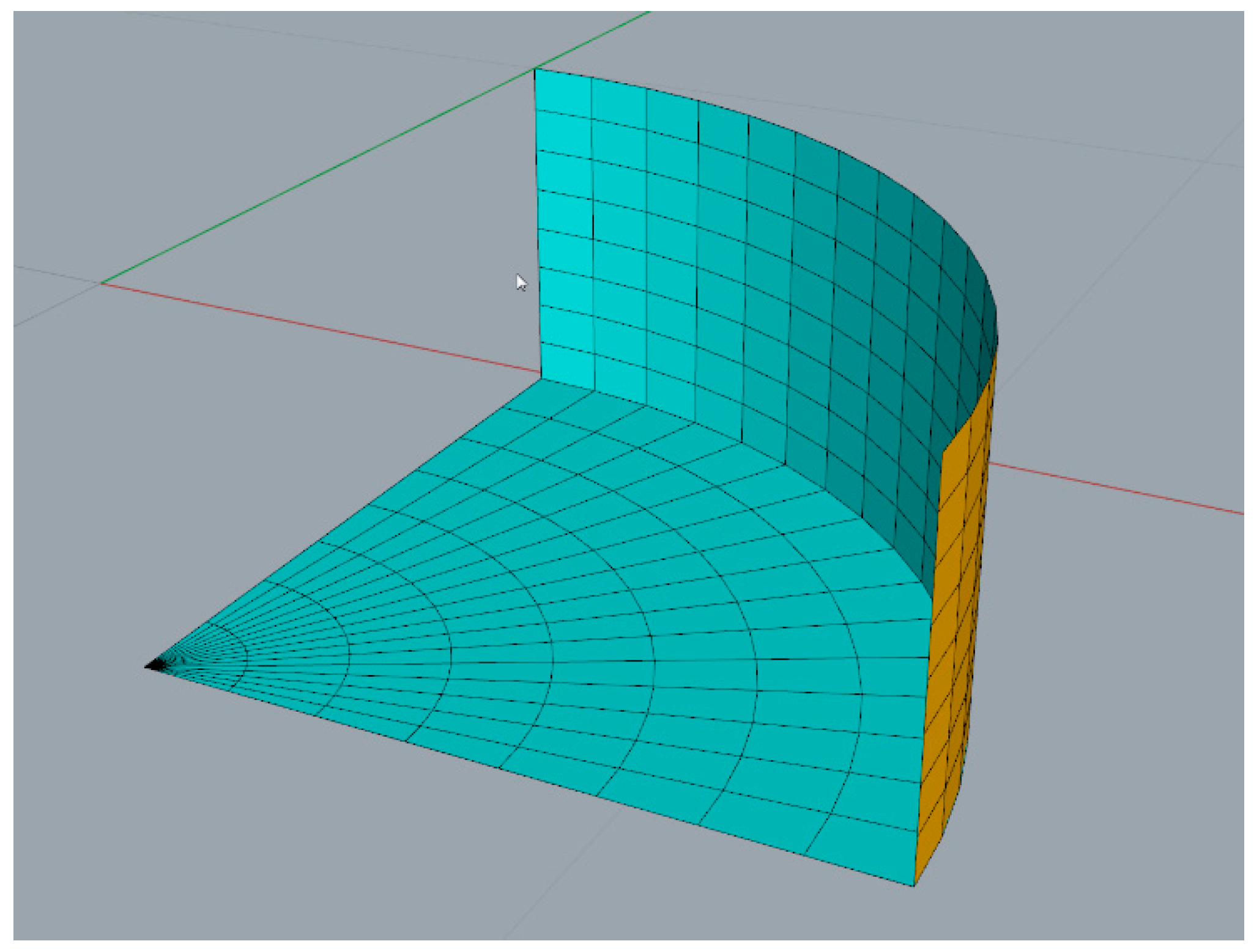
4.1. Computation of an Analytical Geometry for Verification

A numerical benchmark case is performed on a floating ellipsoid (since the geometry of which can be precisely expressed) to demonstrate the validity of the developed solver. The geometry is firstly meshed by 20 × 20 panels (20 in longitude and 20 in latitude directions) on the immersed body surface, and additional 10 × 20 panels (10 in longitude and 20 in latitude directions) at the interior waterplane to suppress the so-called “irregular frequencies”. To check its symmetrical property, the other two meshes that have one symmetry plane and two symmetry planes are also employed for comparison in altogether 300 panels and 150 panels, respectively. All the meshes are shown in Figure 6, where lengths of the major axis and the minor axis of the ellipsoid are L/A = 1.0 and B/A = 0.5, respectively, and normalized by the unit amplitude of a regular incident wave coming towards the positive x-direction.
Figure 7 shows the effect of the irregular frequencies. In the vicinity of the irregular frequencies, un-removal of them results in sharp leaps and declines within small intervals, leading to substantial numerical errors. In contrast, the “Removed” method based on the modified boundary integral equation obtains smooth results in the entire neighborhood. It is interesting to see that the irregular frequencies are different in the horizontal and the vertical exciting forces since they correspond to solutions of the interior sloshing problem in different modes.
A comparison of the hydrodynamic coefficients against the normalized length v L is given in Figure 8. The rotation center of the torque is defined at the origin. The present numerical results show good coincidence with the analytical results obtained by Kudoh (1978) [25], in both the translational mode and rotational mode. Meanwhile, the comparison also shows that although utilization of the symmetrical properties decreases the computation burden, it does not affect the accuracy of results.

4.2. Computation of a Truncated Circular Cylinder

Circular cylinder is another common element in the offshore structures. In this test, a truncated circular cylinder with a radius of 1.0 m and a draft of 0.5 m is chosen as a basic example, as displayed in Figure 9. Thanks to its two symmetry planes, a quarter of the cylinder is discretized into 16 × 8 × 8 constant panels (16 in circumferential, 8 in radial, and 8 in vertical directions) of a quadrilateral or triangular element shape. To remove the irregular frequencies, the water-plane area is discretized into 16 × 8 constant panels (16 in circumferential, and 8 in radial directions). Computations are performed using the HAMS solver as well as the commercial software WAMIT®, and Hydrostar®, for comparison.
Hydrodynamic quantities involving added mass and wave damping are compared between the computation results derived from the three software. Dimensional results are shown against the wave angular frequency ω in Table 1 and Table 2. In Table 1, the computations are carried out in the deep water, while in Table 2, the water is shallow with a depth of h = 1.0 m. The tables illustrate that no matter if the water depth is infinite or finite, the results from HAMS and WAMIT® are much closer between each other against the wave frequency, while those from Hydrostar® are a bit shifted away. It may possibly be due to Hydrostar® being based on the source distribution method while the other two are based on the mixed source/dipole method in calculating the wave potentials.

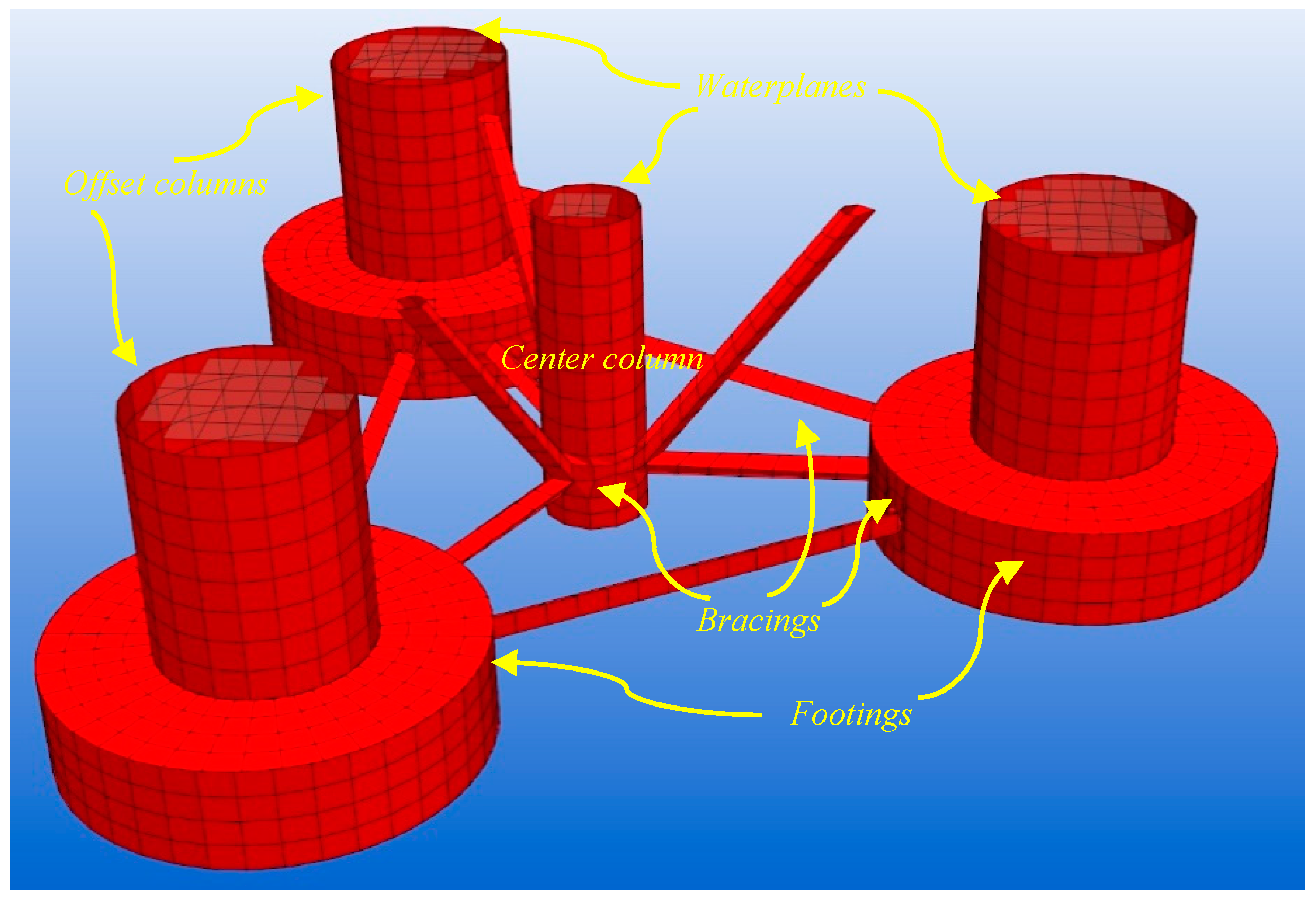
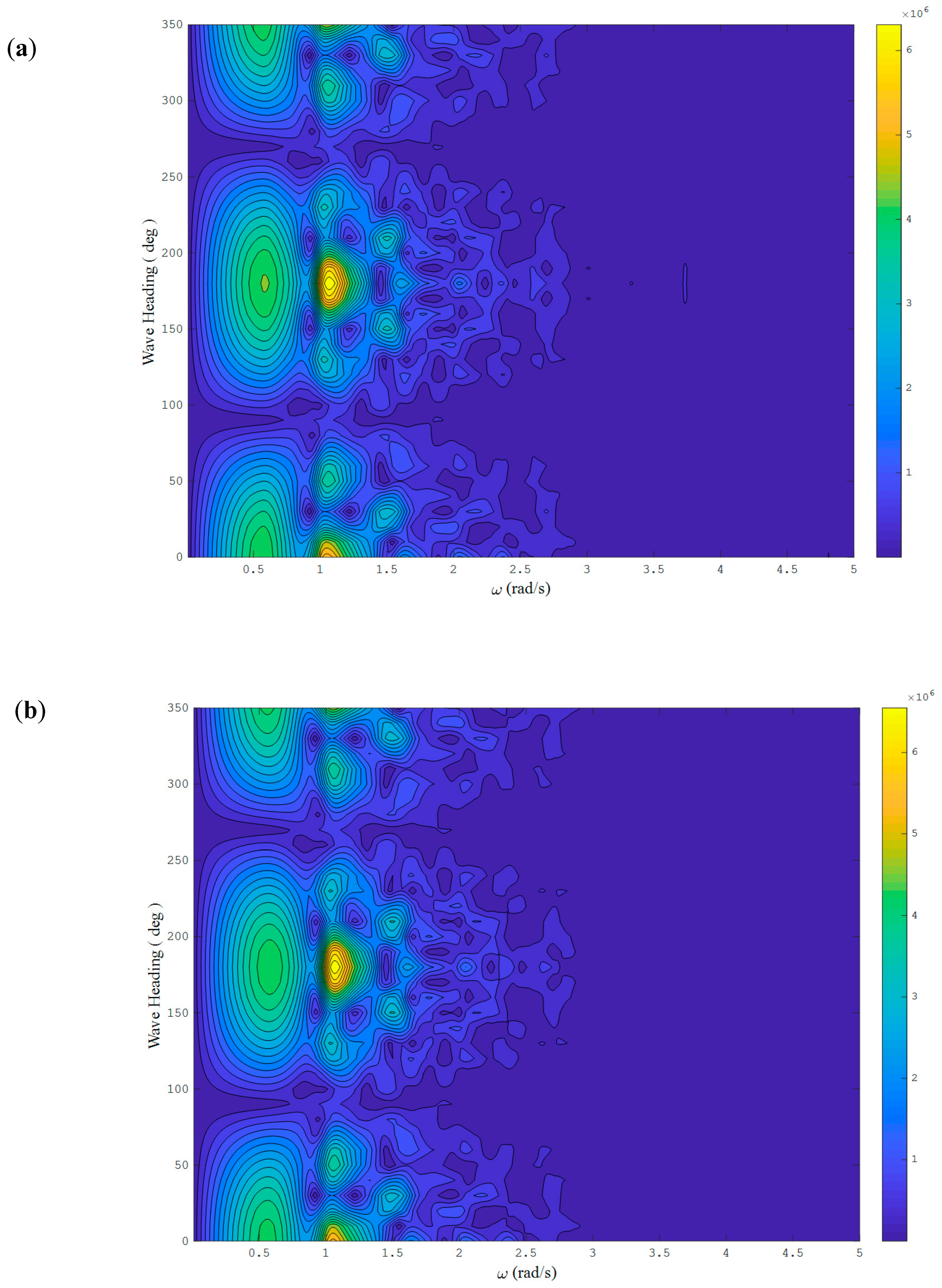
4.3. Computation of a Complex Marine Structure

To illustrate the capabilities of the HAMS preprocessor in the wave-structure interaction analysis, the floating foundation of the complex OC4 DeepCwind semisubmersible floating wind turbine is presented herein as a benchmark test in practice. The platform consists of a central column, three outer offset columns, and a host of slender bracings to connect between the columns and make the floating structure sufficiently stiff. Geometrical specifications of the DeepCwind semi-submersible are found in Ref. [26].
A hydrodynamic mesh is only generated for the wetted part of the floater, and the waterplane at the cross-sections of the columns intersecting the mean sea surface. Around 3000 panels are chosen as an appropriate number of panels for the following computation, as displayed in Figure 10. Each of the three footings is discretized into 38 × 8 × 4 constant panels (38 in circumferential, 8 in radial, and 4 in vertical directions) of a quadrilateral or triangular element shape. Each of the three outer offset columns and the central column are discretized into 20 × 4 × 8 panels and 12 × 2 × 12 panels, respectively. The bracings are also meshed by sufficiently dense panels. A symmetry plane x-z is applied to remarkably reduce the computation time. Computation results using the same hydrodynamic mesh from the commercial software Hydrostar® are also given to validate the present numerical results.
Hydrostatic properties including displacement, center of buoyancy, water plane, restoring, etc., of the OC4 DeepCwind floater have been calculated by HAMS and Hydrostar®, as displayed in Table 3. These properties are evaluated based on the input hydrodynamic mesh of the immersed part of the floater. The comparison shows that the results generated by the two software are very close to each other, with quite small relative errors. A sound accuracy of the hydrostatic properties ensures a good prediction of the motion responses in subsequent calculations.
Figure 11 shows distributions of the wave excitation force in the x-direction on the OC4 DeepCwind floater with respect to the wave angular frequency and wave headings. Firstly, it is seen that the distributions computed by respectively HAMS and Hydrostar® are in good agreement with each other. Secondly, due to the symmetry of the OC4 DeepCwind floater, the distributions are symmetric with respect to the line of the wave heading β = 180 ° . It should be noted that there are several major regions where the floater is acted on significantly by the wave force. The maximum value occurs at the region of 170 ° < β <   190 ° and 1.0 < ω <   1.2 . Outputting such distributions of wave excitation forces may be of great importance to the design of such floaters in practice [27].
Figure 12 shows the analysis of response amplitude operators (RAOs) on the motions of the OC4 DeepCwind floating wind turbine in no-wind and parking condition, and a comparison between the present results and those computed by the commercial software Hydrostar®. The floating wind turbine is moored with three catenary lines at the near bottom of the outer columns spread symmetrically about the platform z-axis [26]. The mooring system is considered in the calculation, and the mooring stiffness matrix is obtained via linearization of the mooring system. The motion RAOs are measured by the motion response amplitude over the incident wave amplitude. The RAOs are plotted in the logarithmic coordinate to clearly show the comparison. It is seen that the two results basically coincide well with each other, except for some tiny differences below the scale of the 10−4 degree. The peaks at the resonance region (0.0 < ω < 0.5) predicted by the two software packages are also in quite good agreement. The motion RAOs generally decreases with the increase of the wave angular frequency to a negligible level when the wave angular frequency exceeds 2.0.
The computation time and the speed-up ratio of the present case against the number of OpenMP threads for each wave frequency are shown in Figure 13. The elapsed time is an average of the computation time for 60 wave frequencies. The speedup ratio is calculated by the ratio of the computation time of a single thread over that of Nt OpenMP threads. It is found that the computation time in either finite depth or infinite depth decreases with the increase of the number of threads. The computation time in finite depth is a bit less than two times of that in infinite depth. For instance, when eight threads are used, the computation time for every frequency is 9.10 s for the finite depth and 4.86 s for the infinite depth due to the fact that the calculation of the finite depth Green’s function is much more time-consuming than that of infinite depth. The speedup ratio generally increases proportionally with the number of threads but seems to drop a bit when the number of threads exceeds six. Moreover, it is worth noting that the speed-up ratio is less than the number of threads because not all of the codes in the solver can be run in parallel, as indicated in Equation (38).

5. Concluding Remarks

A new software is presented herein for analysis of wave-structure interactions in the frequency domain. To give a clear map of how the software has been developed, the background theory as well as its numerical methodologies and techniques have been introduced in detail. The irregular frequencies have been removed based on the partially extended boundary integral equation method, and symmetry properties can be exploited to reduce the computation burden significantly. The free-surface Green’s function is calculated by a combination of series expansions in both infinite depth and finite depth. OpenMP parallelization is employed to speed up computations on multi-core machines. The accuracy and the efficiency of the developed software were confirmed by numerical validations on three benchmark cases of a floating ellipsoid, a truncated circular cylinder and the OC4 DeepCwind semisubmersible floating wind turbine.

Author Contributions

Y.L. designed the code structure, developed the software, performed the computation, and drafted and polished the paper.

Funding

Development of the software was based on the author’s personal interest, but received no specific external funding. A part of the APC (395 CHF) for publishing this paper is funded by the Q-PIT (Kyushu University Platform of Inter/Transdisciplinary Energy Research) Support Program for Young Researchers (Grant Number 18112).

Acknowledgments

The author appreciates many helpful discussions with Bin Teng, Hidetsugu Iwashita, and Masashi Kashiwagi regarding the issues of calculating free-surface Green’s function, removing irregular frequencies, exploiting symmetrical properties, and integrating Rankine terms, etc. The author appreciates the support from Changhong Hu and Makoto Sueyoshi on many other issues when he was undertaking his Ph.D. The author also appreciates Shigeo Yoshida for providing the commercial software Hydrostar® used in the case validations in Section 4.2 and Section 4.3, and Hongzhong Zhu for providing the commercial software WAMIT® used in the case validation in Section 4.2.

Conflicts of Interest

No potential conflict of interest was reported by the author.

Instructions for the software acquisition

An academic version of the software is freely available on contacting the author. The software can read a mesh file in the *.gdf format. Moreover, it is able to output the frequency-domain calculation results to the WAMIT® or the Hydrostar® format.

Nomenclature

APIApplication Programming Interface
BIEMBoundary Integral Equation Method
CFDComputational Fluid Dynamics
GMRESGeneralized Minimum Residual
JONSWAPJoint North Sea Wave Observation Project
LULower–Upper
N-SNavier-Stokes
OpenMPOpen Multi-Processing
RAOResponse Amplitude Operator

References

  1. Li, Y.; Yu, Y.H. A synthesis of numerical methods for modeling wave energy converter-point absorbers. Renew. Sustain. Energy Rev. 2012, 16, 4352–4364. [Google Scholar] [CrossRef]
  2. Li, Y.; Teng, B. Wave Action on Maritime Structures, 3rd ed.; Ocean Press: Beijing, China, 2015. [Google Scholar]
  3. Newman, J.N. Algorithms for free-surface Green function. J. Eng. Math. 1985, 19, 57–67. [Google Scholar] [CrossRef]
  4. Newman, J.N. The approximation of free-surface Green functions. In Wave Asymptotics; Retirement Meeting for Professor Fritz Ursell, University of Manchester; Martin, P.A., Wickham, G.R., Eds.; Cambridge University Press: Cambridge, UK, 1992; pp. 107–135. [Google Scholar]
  5. Telste, J.G.; Noblesse, F. Numerical evaluation of the Green function of water-wave radiation and diffraction. J. Ship Res. 1986, 30, 69–84. [Google Scholar]
  6. Wu, H.; Zhang, C.; Zhu, Y.; Li, W.; Wan, D.; Noblesse, F. A global approximation to the Green function for diffraction radiation of water waves. Eur. J. Mech.-B/Fluids 2017, 65, 54–64. [Google Scholar] [CrossRef]
  7. Chen, X.B. Evaluation de la fonction de Green du probleme de diffraction/radiation en profondeur d’eau finie-une nouvelle méthode rapide et précise, Actes des 4e Journées de l’Hydrodynamique. Nantes (Franc.) 1993, 371–384. [Google Scholar]
  8. Chen, X.B. Hydrodynamics in offshore and naval applications—Part I. In Proceedings of the 6th International Conference on Hydrodynamics, Perth, Australia, 24–26 November 2004. [Google Scholar]
  9. Liu, Y.; Iwashita, H.; Hu, C. A calculation method for finite depth free-surface green function. International. J. Nav. Archit. Ocean Eng. 2015, 7, 375–389. [Google Scholar] [CrossRef]
  10. Liu, Y.; Yoshida, S.; Hu, C.; Sueyoshi, M.; Sun, L.; Gao, J.; Cong, P.; He, G. A reliable open-source package for performance evaluation of floating renewable energy systems in coastal and offshore regions. Energy Convers. Manag. 2018, 174, 516–536. [Google Scholar] [CrossRef]
  11. Saad, Y.; Schultz, M.H. GMRES: A generalized minimal residual algorithm for solving nonsymmetric linear systems. SIAM J. Sci. Stat. Comput. 1986, 7, 856–869. [Google Scholar] [CrossRef]
  12. John, F. On the motion of floating bodies II. Commun. Pure Appl. Math. 1950, 3, 45–101. [Google Scholar] [CrossRef]
  13. Ursell, F. Irregular frequencies and the motion of floating bodies. J. Fluid Mech. 1981, 105, 143–156. [Google Scholar] [CrossRef]
  14. Lee, C.H.; Sclavounos, P.D. Removing the irregular frequencies from integral equations in wave-body interactions. J. Fluid Mech. 1989, 207, 393–418. [Google Scholar] [CrossRef]
  15. Lee, C.H.; Newman, J.N.; Zhu, X. An extended boundary integral equation method for the removal of irregular frequency effects. Int. J. Numer. Methods Fluids 1996, 23, 637–660. [Google Scholar] [CrossRef]
  16. Malenica, S.; Chen, X.B. On the irregular frequencies appearing in wave diffraction-radiation solutions. Int. J. Offshore Polar Eng. 1998, 8, 110–114. [Google Scholar]
  17. Sun, L.; Teng, B.; Liu, C.F. Removing irregular frequencies by a partial discontinuous higher order boundary element method. Ocean Eng. 2008, 35, 920–930. [Google Scholar] [CrossRef] [Green Version]
  18. Kashiwagi, M.; Takagi, K.; Yoshida, H.; Murai, M.; Higo, Y. Fluid Dynamics of Floating Bodies in Practice: Part 1 Numerical Computation Method of the Motion Response Problems; Seisando Press: Tokyo, Japan, 2003. [Google Scholar]
  19. Newman, J.N. Distributions of sources and normal dipoles over a quadrilateral panel. J. Eng. Math. 1986, 20, 113–126. [Google Scholar] [CrossRef]
  20. Lau, S.M.; Hearn, G.E. Suppression of irregular frequency effects in fluid–structure interaction problems using a combined boundary integral equation method. Int. J. Numer. Methods Fluids 1989, 9, 763–782. [Google Scholar] [CrossRef]
  21. Lee, C.H. WAMIT Theory Manual: MIT Report 95-2; Dept. of Ocean Engineering, Massachusetts Institute of Technology: Cambridge, MA, USA, 1995. [Google Scholar]
  22. Chau, F.P. The Second Order Velocity Potential for Diffraction of Waves by Fixed Offshore Structures. Ph.D. Thesis, University College London, London, UK, 1989. [Google Scholar]
  23. Matsui, T.; Kato, K.; Shirai, T. A hybrid integral equation method for diffraction and radiation of water waves by three-dimensional bodies. Comput. Mech. 1987, 2, 119–135. [Google Scholar] [CrossRef]
  24. Kiessling, A. An Introduction to Parallel Programming with OpenMP. In A Pedagogical Seminar; Edinburgh University: Edinburgh, UK, 2009. [Google Scholar]
  25. Kudou, K.; Kobayashi, K. The drifting force acting on a three-dimensional body in waves (2nd Report). J. Soc. Nav. Arch. Jap. 1978, 144, 155–162. [Google Scholar] [CrossRef]
  26. Robertson, A.; Jonkman, J.M.; Masciola, M.; Song, H.; Goupee, A.; Coulling, A.; Luan, C. Definition of the Semisubmersible Floating System for Phase II of OC4; National Renewable Energy Laboratory (NREL): Golden, CO, USA, 2014. [Google Scholar]
  27. McCormick, M.E. Ocean Engineering Mechanics: With Applications; Cambridge University Press: Cambridge, UK, 2009. [Google Scholar]
Figure 1. Definition of the coordinate system in the three-dimensional space. Q denotes the source point on the immersed body boundary SB, and P denotes the field point anywhere in the fluid domain.
Jmse 07 00081 g001
Figure 2. Illustration of the collection method: Collection points are located at the centroid of each panel, and the influence coefficients Sij and Dij between each two of these points are evaluated subsequently.
Jmse 07 00081 g002
Figure 3. Illustration of the local coordinate system of each panel, in triangular shape (a) or quadrilateral shape (b). The origin o normally locates at the centroid of each panel, and the positive ζ-axis points to the normal direction of the panel. The sequence of vertices is arranged in accordance with the normal direction that points into the inside of the body.
Jmse 07 00081 g003
Figure 4. Partitions of the computation domain (a) when the body has unique symmetry and (b) when the body has two symmetries.
Jmse 07 00081 g004
Figure 5. Schematic of the two main OpenMP parallel processes in the HAMS (Hydrodynamic Analysis of Marine Structures) program.
Jmse 07 00081 g005
Figure 6. Mesh of the floating ellipsoid (a) without symmetry in 600 panels; (b) with one symmetry in 300 panels; and (c) with two symmetries in 150 panels.
Jmse 07 00081 g006
Figure 7. Modulus of the complex exciting wave forces of a floating ellipsoid, as a function of the angular wave frequency ω. (a) Horizontal exciting force. (b) Vertical exciting force.
Jmse 07 00081 g007
Figure 8. Added mass and radiation damping coefficients of a floating ellipsoid as a function of the angular wave frequency ω : (a) diagonal terms of the surge added mass and radiation damping due to surge motion and (b) cross terms of the surge added mass and radiation damping due to pitch motion.
Jmse 07 00081 g008
Figure 9. Hydrodynamic mesh of the immersed part of a truncated circular cylinder for use in HAMS, WAMIT®, and Hydrostar®.
Jmse 07 00081 g009
Figure 10. Hydrodynamic mesh of the immersed part of the OC4 DeepCwind floater, for use in HAMS and Hydrostar®.
Jmse 07 00081 g010
Figure 11. Modulus of the wave excitation force in x-direction acting on the OC4 DeepCwind floater as a function of the wave angular frequency ω and wave headings β , computed by (a) HAMS and (b) Hydrostar®, respectively.
Jmse 07 00081 g011
Figure 12. Motion response of the OC4 DeepCwind floating wind turbine in no-wind and parking conditions as a function of the wave angular frequency ω : (a) surge response; (b) heave response; and (c) pitch response. The results denoted by symbols are computed by the commercial software Hydrostar®.
Jmse 07 00081 g012
Figure 13. Computation efficiency of the HAMS solver for each wave frequency against the number of threads in finite and infinite depth, respectively.
Jmse 07 00081 g013
Table 1. Hydrostatic quantities of the truncated circular cylinder calculated by HAMS, WAMIT®, and Hydrostar®, under the infinite water depth.
A11 (kg)B11 (kg/s)
ωHAMSWAMIT®Hydrostar®HAMSWAMIT®Hydrostar®
0.26.7543 × 1026.7568 × 1026.9207 × 1021.7266 × 10−51.7268 × 10−51.8018 × 10−5
0.46.7910 × 1026.7936 × 1026.9587 × 1022.2008 × 10−32.2011 × 10−32.2972 × 10−3
0.66.8554 × 1026.8579 × 1027.0252 × 1023.7342 × 10−23.7344 × 10−23.8977 × 10−2
0.86.9525 × 1026.9549 × 1027.1257 × 1022.7704 × 10−12.7705 × 10−12.8915 × 10−1
17.0898 × 1027.0922 × 1027.2679 × 1021.3046 × 1001.3046 × 1001.3616 × 100
1.27.2764 × 1027.2788 × 1027.4612 × 1024.6032 × 1004.6031 × 1004.8047 × 100
1.47.5214 × 1027.5238 × 1027.7152 × 1021.3292 × 1011.3291 × 1011.3876 × 101
1.67.8308 × 1027.8334 × 1028.0363 × 1023.3087 × 1013.3080 × 1013.4547 × 101
1.88.2032 × 1028.2058 × 1028.4225 × 1027.3328 × 1017.3303 × 1017.6586 × 101
28.6221 × 1028.6241 × 1028.8561 × 1021.4765 × 1021.4757 × 1021.5426 × 102
2.29.0462 × 1029.0476 × 1029.2939 × 1022.7338 × 1022.7317 × 1022.8566 × 102
2.49.4047 × 1029.4056 × 1029.6610 × 1024.6820 × 1024.6770 × 1024.8918 × 102
2.69.6011 × 1029.6010 × 1029.8548 × 1027.4309 × 1027.4201 × 1027.7582 × 102
2.89.5346 × 1029.5338 × 1029.7703 × 1021.0927 × 1031.0906 × 1031.1391 × 103
39.1418 × 1029.1415 × 1029.3441 × 1021.4891 × 1031.4858 × 1031.5488 × 103
Table 2. Hydrostatic quantities of the truncated circular cylinder calculated by HAMS, WAMIT®, and Hydrostar®, under a finite water depth h = 1.0 m.
A11 (kg)B11 (kg/s)
ωHAMSWAMIT®Hydrostar®HAMSWAMIT®Hydrostar®
0.28.3818 × 1028.3854 × 1028.6347 × 1025.9702 × 10−15.9721 × 10−16.2698 × 10−1
0.48.5111 × 1028.5148 × 1028.7701 × 1024.8315 × 1004.8329 × 1005.0754 × 100
0.68.6790 × 1028.6824 × 1028.9452 × 1021.6554 × 1011.6558 × 1011.7395 × 101
0.88.8657 × 1028.8693 × 1029.1401 × 1023.9904 × 1013.9913 × 1014.1945 × 101
19.0548 × 1029.0584 × 1029.3367 × 1027.9279 × 1017.9292 × 1018.3352 × 101
1.29.2291 × 1029.2323 × 1029.5164 × 1021.3917 × 1021.3918 × 1021.4633 × 102
1.49.3720 × 1029.3726 × 1029.6595 × 1022.2390 × 1022.2386 × 1022.3536 × 102
1.69.4581 × 1029.4593 × 1029.7449 × 1023.3699 × 1023.3692 × 1023.5412 × 102
1.89.4700 × 1029.4728 × 1029.7517 × 1024.8075 × 1024.8064 × 1025.0489 × 102
29.3921 × 1029.3948 × 1029.6609 × 1026.5558 × 1026.5535 × 1026.8779 × 102
2.29.2083 × 1029.2108 × 1029.4576 × 1028.5924 × 1028.5877 × 1029.0016 × 102
2.48.9104 × 1028.9127 × 1029.1343 × 1021.0865 × 1031.0857 × 1031.1362 × 103
2.68.4981 × 1028.5006 × 1028.6922 × 1021.3295 × 1031.3283 × 1031.3873 × 103
2.87.9810 × 1027.9838 × 1028.1423 × 1021.5780 × 1031.5761 × 1031.6426 × 103
37.3805 × 1027.3801 × 1027.5047 × 1021.8209 × 1031.8180 × 1031.8902 × 103
Table 3. Hydrostatic properties of the OC4 DeepCwind floater calculated by HAMS and Hydrostar®.
PropertiesHAMSHydrostar®Relative Error
Displacement1.3683 × 104 m31.3683 × 104 m30.00
z-Coordinate of the Buoyancy Center−1.3157 × 101 m−1.3185 × 101 m2.12 × 10−3
Area of the Immersed Body Surface6.5010 × 103 m26.5007 × 103 m24.61 × 10−5
Inner Water Plane Area3.7027 × 102 m23.7128 × 102 m2−2.72 × 10⁻³
Hydrodynamic Restoring in Heave3.7219 × 106 N/m3.7736 × 106 N/m−1.37 × 10−2
Hydrodynamic Restoring in Roll−3.7649 × 10⁸ Nm/rad−3.6278 × 108 Nm/rad3.78 × 10−2
Hydrodynamic Restoring in Pitch−3.7649 × 10⁸ Nm/rad−3.6278 × 108 Nm/rad3.78 × 10−2

