Characterizing Wave Shape Evolution on an Ebb-Tidal Shoal


Abstract
:1. Introduction
2. Methodology
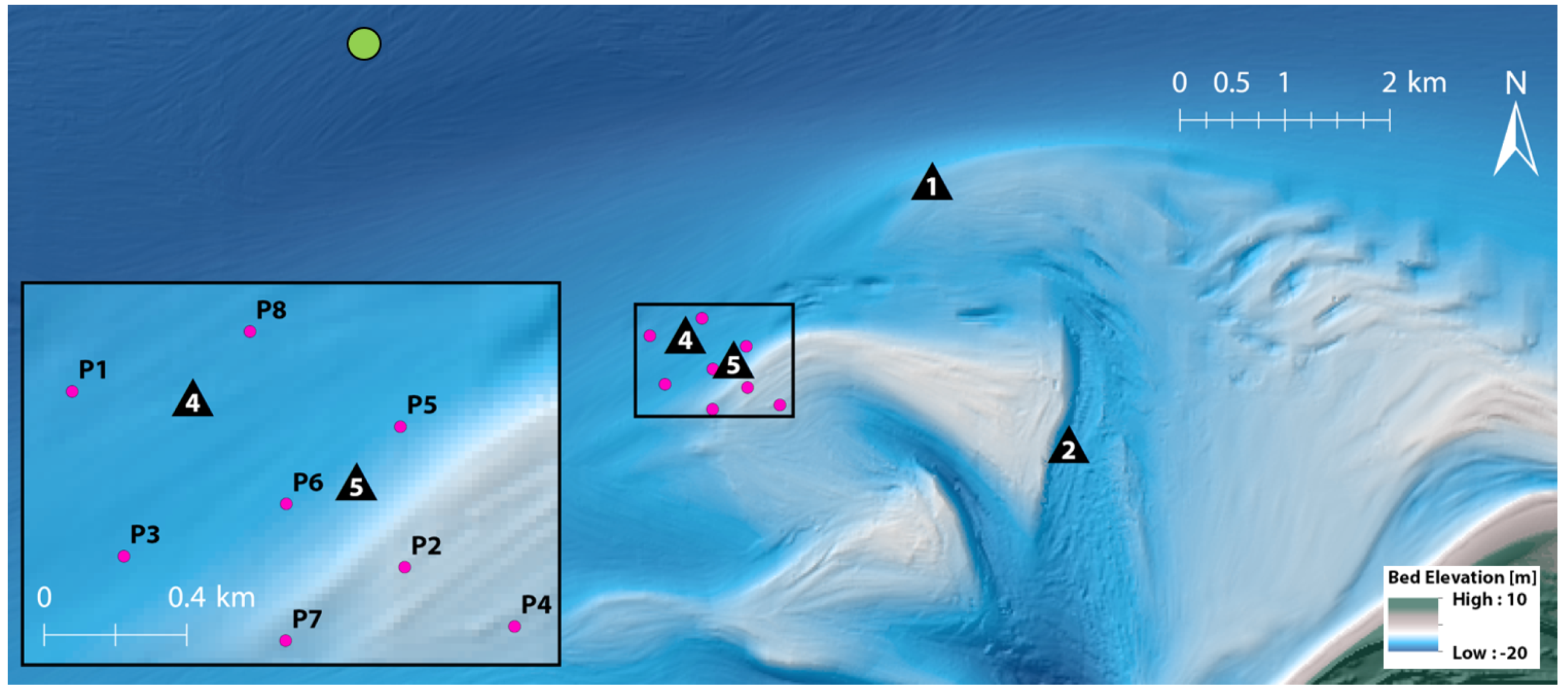
2.1. Field Campaign
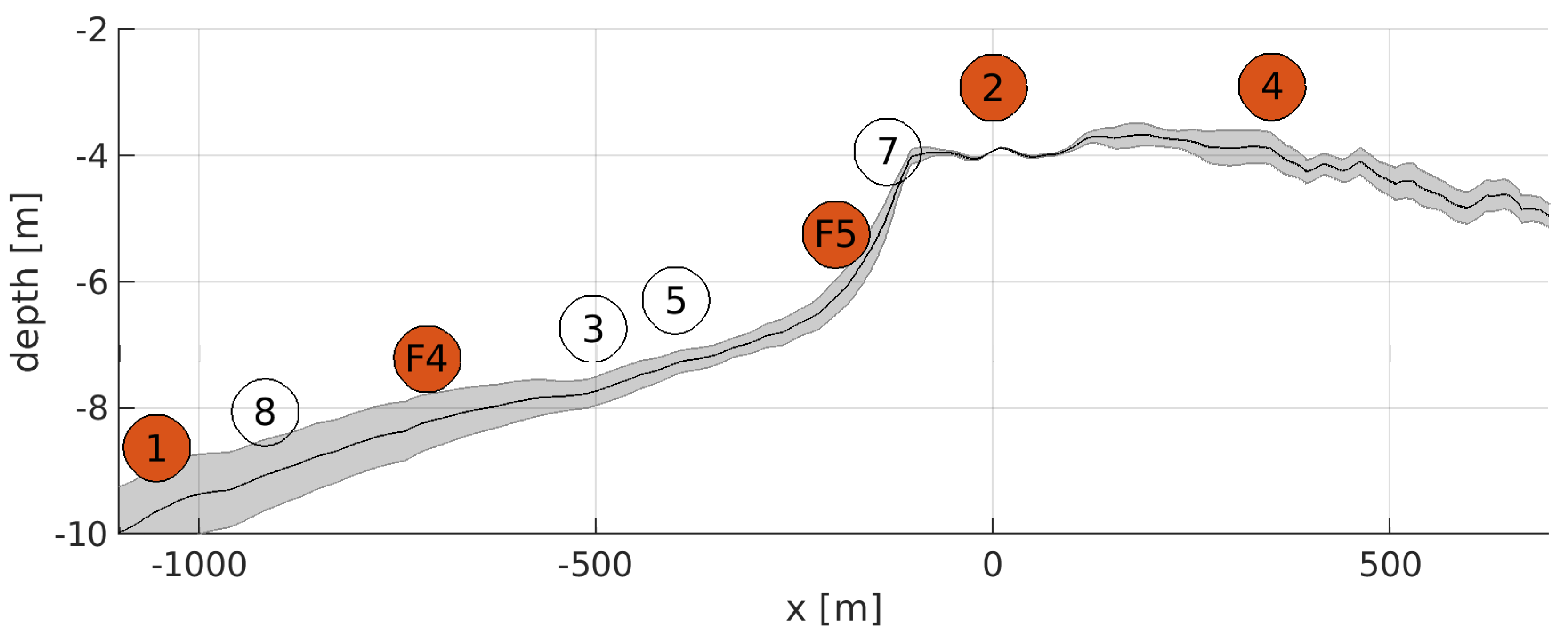
- Shelf: PS1, PS8, F4, and PS3. These sensors were at the milder shelf in mean depths between 10.5 and 8 m.
- Seaward slope: PS5, PS7, and F5. These sensors were at the steeper seaward edge of the shoal in mean depths between 8 and 5 m.
- Shoal: PS2 was at the transition between the seaward slope and the flat top of the shoal.
- Landward slope: PS4 was at the basin end slope of the shoal. It was 300 m more landward than PS2 in a region where the depth starts increasing after the shallowest point, which was located between PS4 and PS2.
2.2. Data Processing
2.2.1. Velocity
2.2.2. Pressure
2.2.3. Calculation of Nonlinear Parameters
2.2.4. Estimation of Near-Bed Velocity Time Series from Pressure Signals
2.3. Depth-Averaged Currents
3. Results
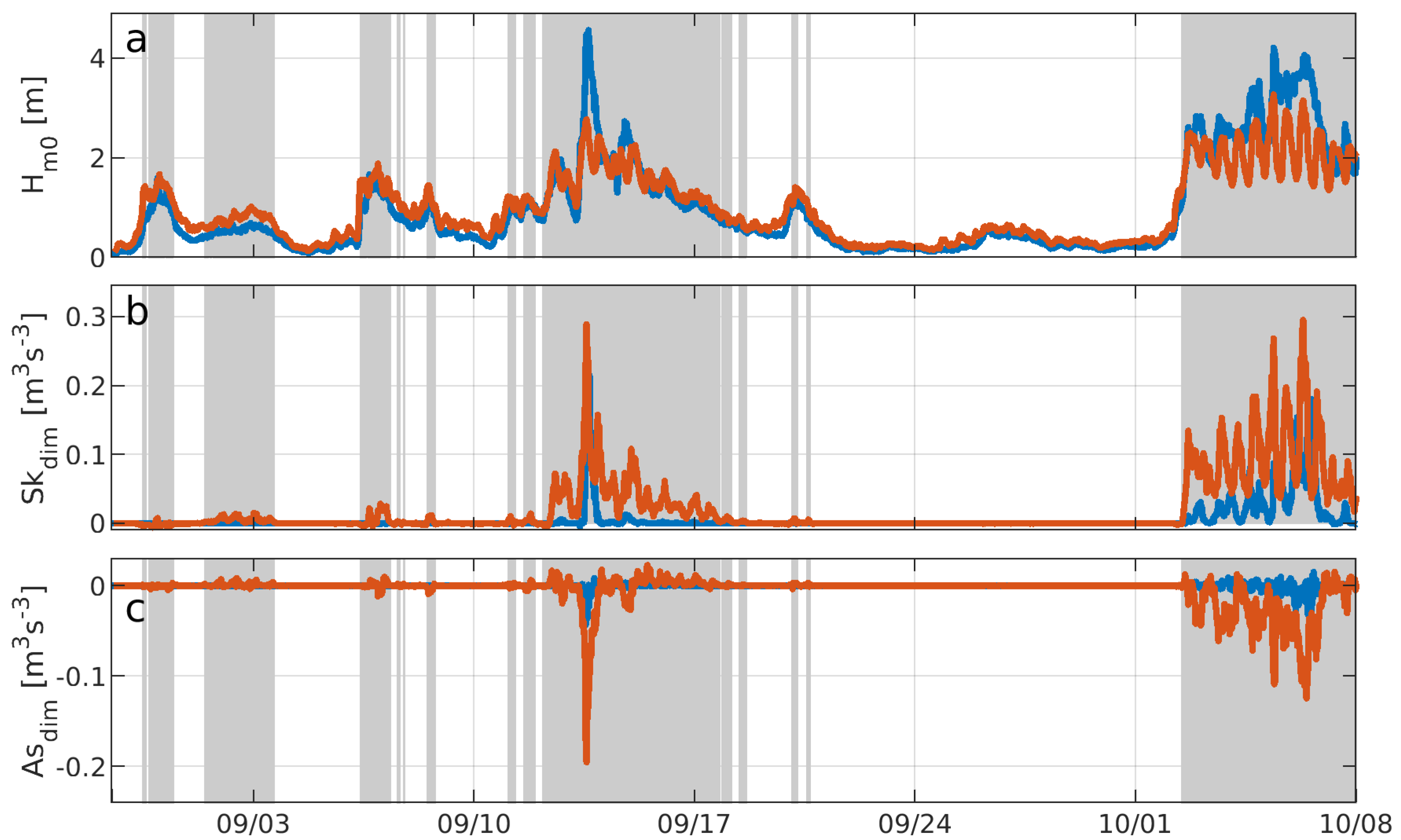
3.1. Data Overview and Selection
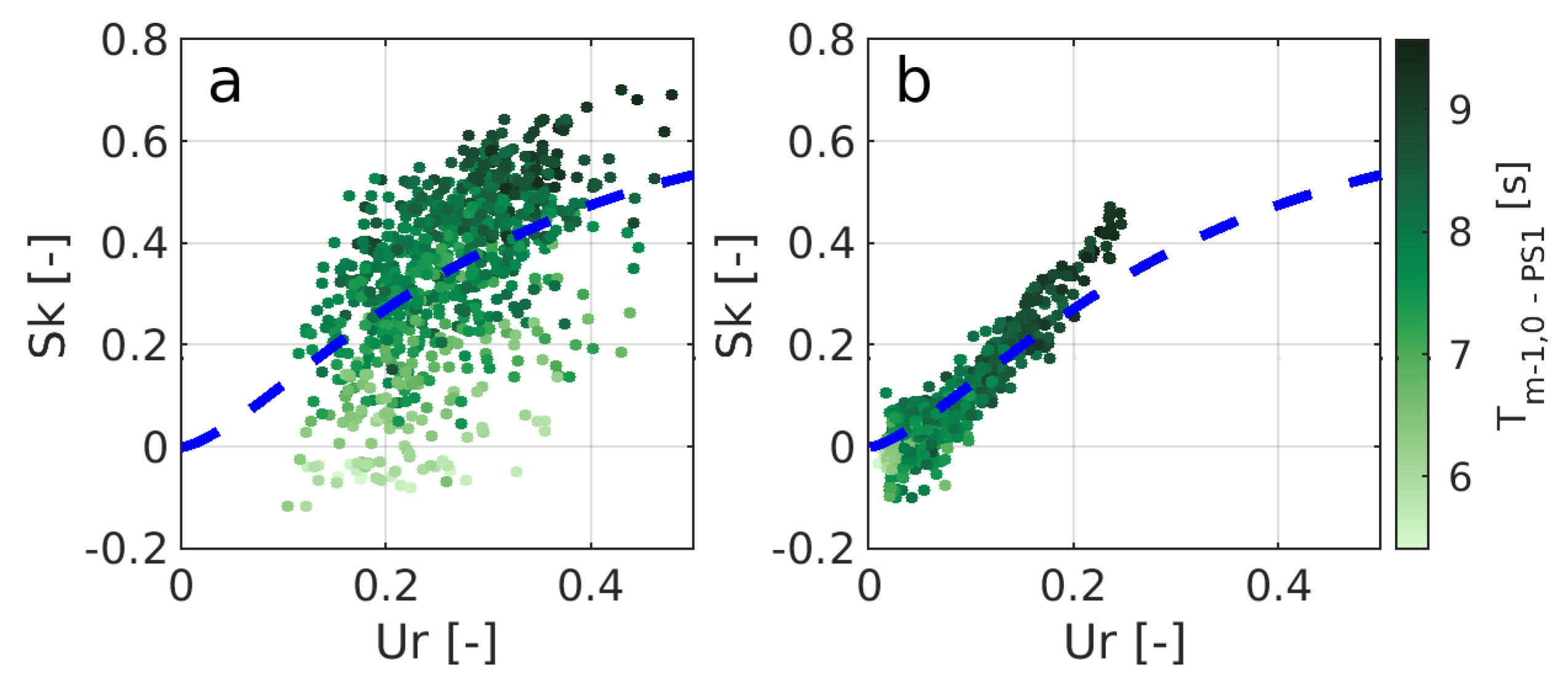
3.2. Dependance of Wave Shape Parameters on the Local Ursell Number
3.3. Role of Wave Transformation
3.3.1. Variability Caused by Wave Breaking
3.3.2. Variability Caused by Nonlinear Energy Transfer Rate
3.3.3. Variability Caused by Currents
4. Discussion
4.1. Relevance in Morphodynamic Modeling
4.2. Correcting for Delayed Response in Wave Shape
4.3. Future Work
5. Conclusions
Author Contributions
Funding
Acknowledgments
Conflicts of Interest
Abbreviations
| ADCP | Acoustic Doppler Current Profiler |
| F# | Frame with # being the number of the frame |
| PS# | Standalone pressure sensor with # being the number of the pressure sensor |
| RMSE | Root-Mean-Squared-Error |
Appendix A. Validity Delft3D Model


| F1 | F4 | F5 | |
|---|---|---|---|
| (m) | 0.17 | 0.25 | 0.16 |
| (m/s) | 0.13 | 0.12 | 0.13 |
| (m/s) | 0.10 | 0.12 | 0.13 |
References
- Hayes, M.O.; Goldsmith, V.; Hobbs, C.H., III. Offset coastal inlets. In Coastal Engineering 1970; American Society of Civil Engineers: Reston, VA, USA, 1970; pp. 1187–1200. [Google Scholar]
- Oertel, G.F. Sediment transport of estuary entrance shoals and the formation of swash platforms. J. Sediment. Res. 1972, 42, 858–863. [Google Scholar]
- Hayes, M.O. General morphology and sediment patterns in tidal inlets. Sediment. Geol. 1980, 26, 139–156. [Google Scholar] [CrossRef]
- Fitzgerald, D.M. Interactions between the ebb-tidal delta and landward shoreline; Price Inlet, South Carolina. J. Sediment. Res. 1984, 54, 1303–1318. [Google Scholar]
- Finley, R.J. Ebb-tidal delta morphology and sediment supply in relation to seasonal wave energy flux, North Inlet, South Carolina. J. Sediment. Res. 1978, 48, 227–238. [Google Scholar]
- Grant, W.D.; Madsen, O.S. Combined wave and current interaction with a rough bottom. J. Geophys. Res. Ocean. 1979, 84, 1797–1808. [Google Scholar] [CrossRef]
- Nielsen, P. Three simple models of wave sediment transport. Coast. Eng. 1988, 12, 43–62. [Google Scholar] [CrossRef]
- Lesser, G.R.; Roelvink, J.A.; Van Kester, J.A.T.M.; Stelling, G.S. Development and validation of a three-dimensional morphological model. Coast. Eng. 2004, 51, 883–915. [Google Scholar] [CrossRef]
- Warner, J.C.; Sherwood, C.R.; Signell, R.P.; Harris, C.K.; Arango, H.G. Development of a three-dimensional, regional, coupled wave, current, and sediment-transport model. Comput. Geosci. 2008, 34, 1284–1306. [Google Scholar] [CrossRef]
- Chen, J.L.; Hsu, T.J.; Shi, F.; Raubenheimer, B.; Elgar, S. Hydrodynamic and sediment transport modeling of New River Inlet (NC) under the interaction of tides and waves. J. Geophys. Res. Ocean. 2015, 120, 4028–4047. [Google Scholar] [CrossRef]
- Hoefel, F.; Elgar, S. Wave-induced sediment transport and sandbar migration. Science 2003, 299, 1885–1887. [Google Scholar] [CrossRef]
- Elgar, S.; Guza, R.T. Observations of bispectra of shoaling surface gravity waves. J. Fluid Mech. 1985, 161, 425–448. [Google Scholar] [CrossRef]
- Boechat Albernaz, M.; Ruessink, G.; Jagers, B.; Kleinhans, M. Effects of Wave Orbital Velocity Parameterization on Nearshore Sediment Transport and Decadal Morphodynamics. J. Mar. Sci. Eng. 2019, 7, 188. [Google Scholar] [CrossRef]
- Stive, M.J.F. A model for cross-shore sediment transport. In Coastal Engineering 1986; American Society of Civil Engineers: Reston, VA, USA, 1987; pp. 1550–1564. [Google Scholar]
- Roelvink, J.A.; Stive, M.J.F. Bar-generating cross-shore flow mechanisms on a beach. J. Geophys. Res. Ocean. 1989, 94, 4785–4800. [Google Scholar] [CrossRef]
- Drake, T.G.; Calantoni, J. Discrete particle model for sheet flow sediment transport in the nearshore. J. Geophys. Res. Ocean. 2001, 106, 19859–19868. [Google Scholar] [CrossRef]
- Doering, J.C.; Bowen, A.J. Parametrization of orbital velocity asymmetries of shoaling and breaking waves using bispectral analysis. Coast. Eng. 1995, 26, 15–33. [Google Scholar] [CrossRef]
- Ruessink, B.G.; Ramaekers, G.; Van Rijn, L.C. On the parameterization of the free-stream non-linear wave orbital motion in nearshore morphodynamic models. Coast. Eng. 2012, 65, 56–63. [Google Scholar] [CrossRef]
- Rocha, M.; Silva, P.; Michallet, H.; Abreu, T.; Moura, D.; Fortes, J. Parameterizations of wave nonlinearity from local wave parameters: A comparison with field data. J. Coast. Res. 2013, 65, 374–379. [Google Scholar] [CrossRef]
- Rocha, M.V.L.; Michallet, H.; Silva, P.A. Improving the parameterization of wave nonlinearities—The importance of wave steepness, spectral bandwidth and beach slope. Coast. Eng. 2017, 121, 77–89. [Google Scholar] [CrossRef]
- Dibajnia, M.; Moriya, T.; Watanabe, A. A representative wave model for estimation of nearshore local transport rate. Coast. Eng. J. 2001, 43, 1–38. [Google Scholar] [CrossRef]
- Norheim, C.A.; Herbers, T.H.C.; Elgar, S. Nonlinear evolution of surface wave spectra on a beach. J. Phys. Oceanogr. 1998, 28, 1534–1551. [Google Scholar] [CrossRef]
- Dong, G.; Chen, H.; Ma, Y. Parameterization of nonlinear shallow water waves over sloping bottoms. Coast. Eng. 2014, 94, 23–32. [Google Scholar] [CrossRef]
- Filipot, J.F. Investigation of the bottom-slope dependence of the nonlinear wave evolution toward breaking using SWASH. J. Coast. Res. 2015, 32, 1504–1507. [Google Scholar]
- Groeneweg, J.; van der Westhuysen, A.; van Vledder, G.; Jacobse, S.; Lansen, J.; van Dongeren, A. Wave modelling in a tidal inlet: Performance of SWAN in the Wadden Sea. In Coastal Engineering 2008: (In 5 Volumes); World Scientific: Singapore, 2009; pp. 411–423. [Google Scholar]
- Rusu, L.; Bernardino, M.; Soares, C.G. Modelling the influence of currents on wave propagation at the entrance of the Tagus estuary. Ocean. Eng. 2011, 38, 1174–1183. [Google Scholar] [CrossRef]
- van Prooijen, B.C.; Tissier, M.F.S.; de Wit, F.P.; Pearson, S.G.; Brakenhoff, L.B.; van Maarseveen, M.C.G.; van der Vegt, M.; Mol, J.W.; Kok, F.; Holzhauer, H.; et al. Measurements of Hydrodynamics, Sediment, Morphology and Benthos on Ameland Ebb-Tidal Delta and Lower Shoreface. Earth Syst. Sci. Data 2019. in preparation. [Google Scholar]
- van Weerdenburg, R.J.A. Exploring the Relative Importance of Wind for Exchange Processes around a Tidal Inlet System: The Case of Ameland Inlet. Master’s Thesis, Delft University of Technology, Delft, The Netherlands, 2019. [Google Scholar]
- Elgar, S.; Raubenheimer, B.; Guza, R.T. Quality control of acoustic Doppler velocimeter data in the surfzone. Meas. Sci. Technol. 2005, 16, 1889. [Google Scholar] [CrossRef]
- Goring, D.G.; Nikora, V.I. Despiking acoustic Doppler velocimeter data. J. Hydraul. Eng. 2002, 128, 117–126. [Google Scholar] [CrossRef]
- Mori, N.; Suzuki, T.; Kakuno, S. Noise of acoustic Doppler velocimeter data in bubbly flows. J. Eng. Mech. 2007, 133, 122–125. [Google Scholar] [CrossRef]
- Nederhoff, C.M.; Schrijvershof, R.A.; Tonnon, P.K.; Van Der Werf, J.J.; Elias, E.P.L. Modelling Hydrodynamics in the Ameland Inlet as a Basis for Studying Sand Transport. In The Proceedings of the Coastal Sediments 2019; World Scientific: Singapore, 2019. [Google Scholar]
- Elgar, S.; Guza, R.T.; Raubenheimer, B.; Herbers, T.H.C.; Gallagher, E.L. Spectral evolution of shoaling and breaking waves on a barred beach. J. Geophys. Res. Ocean. 1997, 102, 15797–15805. [Google Scholar] [CrossRef] [Green Version]
- Battjes, J.; Stive, M. Calibration and verification of a dissipation model for random breaking waves. J. Geophys. Res. Ocean. 1985, 90, 9159–9167. [Google Scholar] [CrossRef]
- Hasselmann, K. On the non-linear energy transfer in a gravity-wave spectrum Part 1. General theory. J. Fluid Mech. 1962, 12, 481–500. [Google Scholar] [CrossRef]
- Reniers, A.J.H.M.; De Wit, F.P.; Tissier, M.F.S.; Pearson, S.G.; Brakenhoff, L.B.; Van Der Vegt, M.; Mol, J.; Van Prooijen, B.C. Wave-Skewness and Current-Related Ebb-Tidal Sediment Transport: Observations and Modeling. In The Proceedings of the Coastal Sediments 2019; World Scientific: Singapore, 2019. [Google Scholar]


| Cluster | Location | Depth (m) | Bed Slope (-) | Instrument | Frequency (Hz) |
|---|---|---|---|---|---|
| Shelf | PS1 | 10.4 | 0.004 | PS | 10 |
| PS8 | 9.5 | 0.004 | PS | 10 | |
| F4 | 8.5 | 0.004 | ADCP down | 4 | |
| ADCP up | 1.25 | ||||
| PS3 | 8.2 | 0.002 | PS | 10 | |
| Seaward slope | PS5 | 7.9 | 0.005 | PS | 10 |
| F5 | 6.6 | 0.006 | ADCP down | 4 | |
| ADCP up | 1.25 | ||||
| PS7 | 5.3 | 0.009 | PS | 10 | |
| Shoal | PS2 | 4.3 | 0.011 | PS | 10 |
| Landward slope | PS4 | 4.6 | −0.002 | PS | 10 |
| Other | F1 | 6.6 | 0.009 | ADCP down | 4 |
| ADCP up | 1.25 |
| Location | ||
|---|---|---|
| PS1 | 0.89 | 0.03 |
| PS8 | 0.88 | 0.05 |
| F4 | 0.87 | 0.10 |
| PS3 | 0.89 | 0.07 |
| PS5 | 0.91 | 0.29 |
| F5 | 0.87 | 0.47 |
| F1 | 0.83 | 0.36 |
| PS7 | 0.76 | 0.74 |
| PS4 | 0.28 | 0.01 |
| PS2 | 0.13 | 0.05 |
| Location | PS1 | PS8 | F4 | PS3 | PS5 | F5 | PS7 | PS2 |
|---|---|---|---|---|---|---|---|---|
| (m) | 0 | 0.25 | 0.2 | 0.2 | 0 | 1.1 | 0.8 | 0.85 |
| d (m) | 10.4 | 9.5 | 8.5 | 8.2 | 7.9 | 6.6 | 5.3 | 4.3 |
| bed slope (-) | 0.004 | 0.004 | 0.004 | 0.002 | 0.005 | 0.006 | 0.009 | 0.011 |
© 2019 by the authors. Licensee MDPI, Basel, Switzerland. This article is an open access article distributed under the terms and conditions of the Creative Commons Attribution (CC BY) license (http://creativecommons.org/licenses/by/4.0/).
Share and Cite
de Wit, F.; Tissier, M.; Reniers, A. Characterizing Wave Shape Evolution on an Ebb-Tidal Shoal. J. Mar. Sci. Eng. 2019, 7, 367. https://doi.org/10.3390/jmse7100367
de Wit F, Tissier M, Reniers A. Characterizing Wave Shape Evolution on an Ebb-Tidal Shoal. Journal of Marine Science and Engineering. 2019; 7(10):367. https://doi.org/10.3390/jmse7100367
Chicago/Turabian Stylede Wit, Floris, Marion Tissier, and Ad Reniers. 2019. "Characterizing Wave Shape Evolution on an Ebb-Tidal Shoal" Journal of Marine Science and Engineering 7, no. 10: 367. https://doi.org/10.3390/jmse7100367