Tidal Variation in Cohesive Sediment Distribution and Sensitivity to Flocculation and Bed Consolidation in An Idealized, Partially Mixed Estuary

Abstract

Particle settling velocity and erodibility are key factors that govern the transport of sediment through coastal environments including estuaries. These are difficult to parameterize in models that represent mud, whose properties can change in response to many factors, including tidally varying suspended sediment concentration (SSC) and shear stress. Using the COAWST (Coupled Ocean-Atmosphere-Wave-Sediment Transport) model framework, we implemented bed consolidation, sediment-induced stratification, and flocculation formulations within an idealized two-dimensional domain that represented the longitudinal dimension of a micro-tidal, muddy, partially mixed estuary. Within the Estuarine Turbidity Maximum (ETM), SSC and median floc diameter varied by a factor of four over the tidal cycle. Downstream of the ETM, the median floc size and SSC were several times smaller and showed less tidal variation (~20% or less). The suspended floc distributions only reached an equilibrium size as a function of SSC and shear in the ETM at peak tidal flow. In general, flocculation increased particle size, which reduced SSC by half in the ETM through increased settling velocity. Consolidation also limited SSC by reduced resuspension, which then limited floc growth through reduced SSC by half outside of the ETM. Sediment-induced stratification had negligible effects in the parameter space examined. Efforts to lessen the computation cost of the flocculation routine by reducing the number of size classes proved difficult; floc size distribution and SSC were sensitive to specification of size classes by factors of 60% and 300%, respectively.

1. Introduction

1.1. Motiviation

Estuaries are valuable coastal ecosystems that provide habitat and nursery services to many fishery species, including finfish, crustaceans, and mollusks. In estuaries, freshwater interacts with saline water and mixing can be dominated by waves, tides, riverine input or any combination [1,2]. This leads to complex hydrodynamic conditions with a broad range in spatial and temporal variability [3,4], such as those driven by tidal asymmetries, spring-neap cycles, and seasonal fluctuations in river discharge [5]. The Estuarine Turbidity Maximum (ETM) is a key feature of partially mixed estuaries that occurs at the convergence of freshwater and sea water, which can trap sediment leading to a peak in suspended sediment concentration (SSC), and moves with changes in hydrodynmic conditions [6]. Thus, understanding the processes that are critical to maintaining healthy estuarine environments is challenging.

Muds that are comprised of higher percentages of clays and silts typically dominate estuarine suspended sediments, and the distribution of these sediments impacts water quality, contaminant transport, and navigation [6]. Elevated SSC in surface waters limits light availability for phytoplankton and submerged aquatic plants [7,8]. It should be noted that this study does not address sandy sediments nor the effects of sand on the behavior of muddy sediments. In macrotidal estuaries, sediments within the channel bed are often dominated by sands [9,10] and the fate of sand is also essential to the evolution and stability of deltaic estuaries [11,12,13]. Thus, this study most directly applies to regions upstream from the mouths of micro- to low-mesotidal estuaries, where the surficial sediments in the main channel are dominated by mud. Such systems are especially common along the US Atlantic coast and include, for example, the Satilla [14], Ashepoo [15], James [16], York [17], Rappahannock [18], Potomac [19], Delaware [8], and Hudson [20].

The cohesive nature of mud allows sediment to be transported as aggregated particles; these aggregates can absorb contaminants thereby influencing the dispersal of contaminates [21]. Recent research in response to the Deepwater Horizon spill in the Gulf of Mexico showed that the aggregation processes of muds was important for predicting the fate of hydrocarbon contaminants in marine systems, as it can combine with suspended sediment to form “OMAs” (oil-mineral-aggregates) that settle to the seafloor [22,23]. Additionally, the formation of fast-settling flocs (aggregated muddy particles; [24]) reduces SSC in surface waters. Other human activities, such as dredging to maintain shipping channels in estuaries, change the distribution of sediment. As long as dredging remains a practice, an understanding of how mud is transported is required to determine ideal locations for dredge materials that lowers environmental impacts, limits channel infilling and reduces the overall costs [25,26]. Therefore, innovative methods for predicting cohesive sediment transport are needed and would improve our understanding and ability to reduce human impacts in these systems.

In 2010, 39 percent of the U.S. population lived in coastal regions; this number and the resulting human impacts are expected to increase [27]. However, since 2010 in Virginia, USA alone, more than $350 million has been invested in reducing nonpoint source pollution and improve water quality [28]. Regulatory managers that are responsible for allocating funds to handle environmental issues use numerical models to provide insight into the impacts on coastal aquatic systems due to changes in land development [29,30], nutrient loads and their reduction [31], climate change [32], as well as numerous other factors. In addition, these models allow scientists to test hypotheses over a variety of temporal and spatial scales, and isolate the impacts of individual processes that cannot be separated in observations [33]. For the Chesapeake Bay, USA, in particular, models have aided in the development of reduced nutrient loads needed to improve water quality and the evaluation of the confidence of these estimates [31,34,35].

1.2. Flocculation, Bed Consolidation, and Sediment-Induced Stratification

The flocculation or deflocculation of fine-grained sediments (i.e., the aggregation or dissaggreation of muddy sediment within the water column) leads to variability in suspended sediment properties such as floc size, shape, and density; producing settling velocities that can range over orders of magnitude [36,37]. For example, flocs observed by a video settling camera in surface waters of the York River estuary, USA, had equivalent spherical diameters that ranged from ~30–500 μm, with settling velocities ranging from ~0.06–3 mm s⁻¹, and exhibited a systematic decrease in floc densities with increasing diameter [38]. Other studies have measured floc sizes greater than 1000 μm [39]; specifically, in the Tamar estuary floc diameters were measured as large as 2200 μm [40]. These properties influence the vertical distribution and the residence time of flocs in the water column as well as their horizontal transport. The local conditions such as the amount of biological secretions present, SSC of both muds and sand, salinity, and hydrodynamics impact floc properties [6,41,42].

Modeling the transport of flocs has been appoached in several different ways, from using constant settling velocities obtained from observations for a single size or set of size classes [43,44,45] to predicting median size or other statistical properties of the size distribution including shifts in the size distribution with a set of population balance equations [46,47,48,49,50,51,52]. An equilibrium floc theory predicts median floc sizes using the SSC and shear rates [46,53], whereas other models are more process oriented, but require the user to define additional parameters such as the size and density of primary particles, (i.e., the smallest particles that make up the flocs), the floc fractal dimension (a parameter that describes the characteristic porosity of the flocs as a function of their diameter), and aggregation and break-up efficiencies [49,54]. However, these floc properties can be altered when deposited to the bed by bed consolidation, but the floc size and settling velocity can adjust to the SSC and turbulence within minutes after resuspension [55,56]. The proper estimation of erosional, depositional, and lateral fluxes for cohesive environments requires evaluation of the contribution of aggregation, as well as bed consolidation.

An unconsolidated and easily erodible muddy bed readily supplies sediment to the water column; but over time, the bed may de-water, consolidate, and become less erodible [57,58]. Bed characteristics other than water content such as clay mineralogy, silt-to-clay ratio, sand fraction and organic content can further alter the erodibility of a muddy bed [58,59,60]. The consolidation of the bed, and in some cases the fraction of sand, increase with depth into the bed and can limit the supply of sediment to the water under increased bed stress [59,61,62]. The erosion of mud from the bed is not well correlated with the size of the component particles [58]; thus, numerical models use other techniques for representing the erodibility of the bed in fine-grained environments. The erosion rate is decreased [63,64], or the critical shear stress for erosion may be increased with increased bed density, depth into the bed, and/or age of the bed layer [65,66].

The presence of elevated SSC near the sediment bed creates vertical density stratification [67,68], i.e., sediment-induced stratification, that can dampen turbulence, reducing the bed stress and reducing the upward mixing process while diminishing the amount of sediment eroded and the sediment-carrying capacity of the fluid [69]. If SSC is limited, then the potential for longitudinal transport may be reduced. Reduction of the sediment carrying capacity due to elevated SSC is often incorporated into numerical models by adding parameters into the turbulence closure scheme that reduce mixing with elevated SSC [66,67,70] or reduce the applied bed stress in concert with increases in SSC [71,72]. A more fundamental approach is to add a formulation that incorporates density changes due to SSC into the equation of state (the function that quantifies fluid density) [73,74], and use the combination of water density and SSC stratification in a turbulence closure model to determine the eddy diffusivity. This requires that the hydrodynamic model have sufficiently high vertical resolution to represent the large gradients in SSC that produce the density-induced stratification found near the bed [74].

The implementation of these cohesive sediment processes into numerical models can be challenging, because several of the model coefficients have a large range of possible values [48,58]. Some parameterizations can be informed by local observations; for example, previous implementations of a bed consolidation formulation have fit model parameters based on erosion microcosm field measurements [75,76]. However, in many cases, parameterization of cohesive sediment models remains difficult. Additionally, inclusion of these cohesive processes can significantly add to the computational cost of a sediment transport model. Thus, due to computational limits, many implementations of sediment transport for muddy environments in the past have used simplified forms for flocculation and bed erodibility despite the potential reduction in the model skill and challenges in parameterizing cohesive formulations.

1.3. COAWST

The Coupled Ocean-Atmospheric-Wave-Sediment Transport model (COAWST), incorporates hydrodynamics from the Regional Ocean Modeling System (ROMS) and the Community Sediment Transport Modeling System (CSTMS; [73]). ROMS is a terrain-following, free-surface, hydrostatic primative equation numerical model. ROMS simulates hydrodynamics by solving equations for continuity and conservation of mass and momentum using hydrostatic and Boussinesq assumptions with various initial and boundary conditions defined by the user. It has a large user community and has been described in detail elsewhere, see [73,77,78]. The CSTMS calculates erosion and deposition to the sediment bed and suspended transport of sediment. Sediment is removed from the bed at the user defined rate when the applied stress is greater than the critical shear stress for erosion. The transport of suspended sediment in the water column is estimated by solving the same advection-diffusion equations as used by the hydrodynamic model for salinity and temperature but with an added source/sink term to allow exchange with the sediment bed for individual sediment classes. Specifically, each sediment class has predefined hydrodynamic properties including particle density, settling velocity, and critical shear stress for erosion that have not accounted for cohesive processes until recently; for more details see [73]. Recent CSTMS developments have added cohesive modules for flocculation and bed consolidation; and its seabed layering routines now also account for cohesive, non-cohesive or mixed sediment beds [53].

The new flocculation routine (FLOCMOD) is a population balance module, and the bed consolidation routine increases the critical shear stress for erosion with depth into the sediment bed [53]. FLOCMOD requires flocculation growth and breakup parameters, primary particle size, and fractal dimension [49]. Flocculation parameters are typically chosen to follow field or laboratory studies that provide expected ranges for the associated parameters [38,79,80]. Sediment is entrained into the water column from the bed in CSTMS when the applied bed stress exceeds the critical shear stress for erosion [73,81,82]. The cohesive bed consolidation module specifies additional sediment erodibility parameters that change with depth [65]. In the York River estuary, a field study aided in defining the exponential increase of critical shear stress for erosion with depth into the bed due to consolidation [60]. However, model estimates were particularly sensitive to values that are difficult to obtain from field observations, such as the initial and equilibrium critical shear stress profiles, and the consolidation and swelling timescales [45]. The effect of density-induced stratification from gradients in SSC in CSTMS is implemented using the same approach as [73,74].

The addition of these cohesive sediment routines provides a more complete representation of the processes that are important for suspended transport of muds. The flocculation routine provides a means of examining impacts that are difficult to measure in situ. However, as yet few studies have capitalized on the implementation of a floc population balance model such as FLOCMOD within a community sediment transport model to evaluate the role of cohesive processes in muddy estuaries.

1.4. Objective and Outline of the Study

The objective of this study is therefore to evaluate the performance of the cohesive sediment routines developed in the COAWST modeling system and examine the impact of these cohesive processes on sediment distribution within an idealized, partially mixed estuarine simulation. The sensitivity of the flocculation module to the number of sediment sizes was also examined, because the computational costs increase with the number of sizes. To that end, the goal of this study is to answer the following questions:

• Considering sediment-induced stratification, flocculation dynamics, and bed consolidation, how do these processes impact sediment distribution along a partially mixed estuarine model?
• How does using fewer sediment sizes constrain our ability to represent sediment dynamics in a cohesive sediment environment?

To address these research questions, an idealized model domain was used to assess the effectiveness, sensitivity to parameterization, and computational costs of the CSTMS flocculation and other cohesive sediment formulations. The simplified, idealized domain was chosen because it carries lower computational costs than the more realistic three-dimensional simulation, allowing us to complete systematic testing in a more feasible time frame. Additionally, idealized models can provide insight on first order impacts and interactions without confounding factors such as complex bathymetry and highly variable forcing functions.

Section 2 details the numerical methods and sediment characteristics utilized in this study and the experiments performed. The results and discussion are presented in Section 3, and suggestions for the future handling of flocculation are provided in Section 4. Finally, the study’s conclusions are outlined in Section 5.

2. Materials and Methods

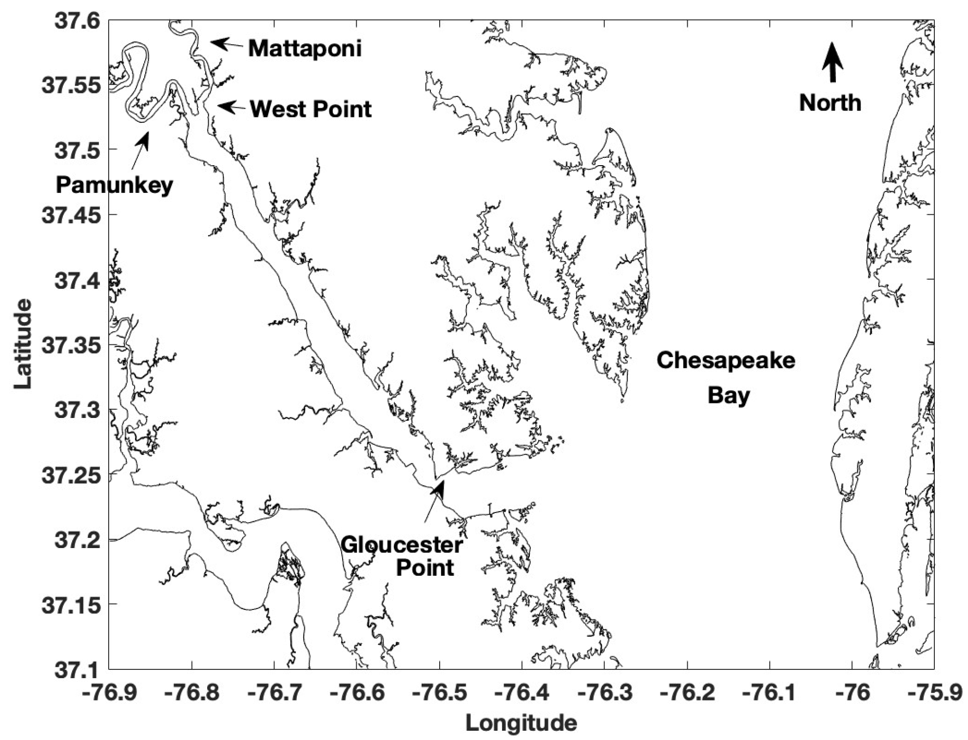
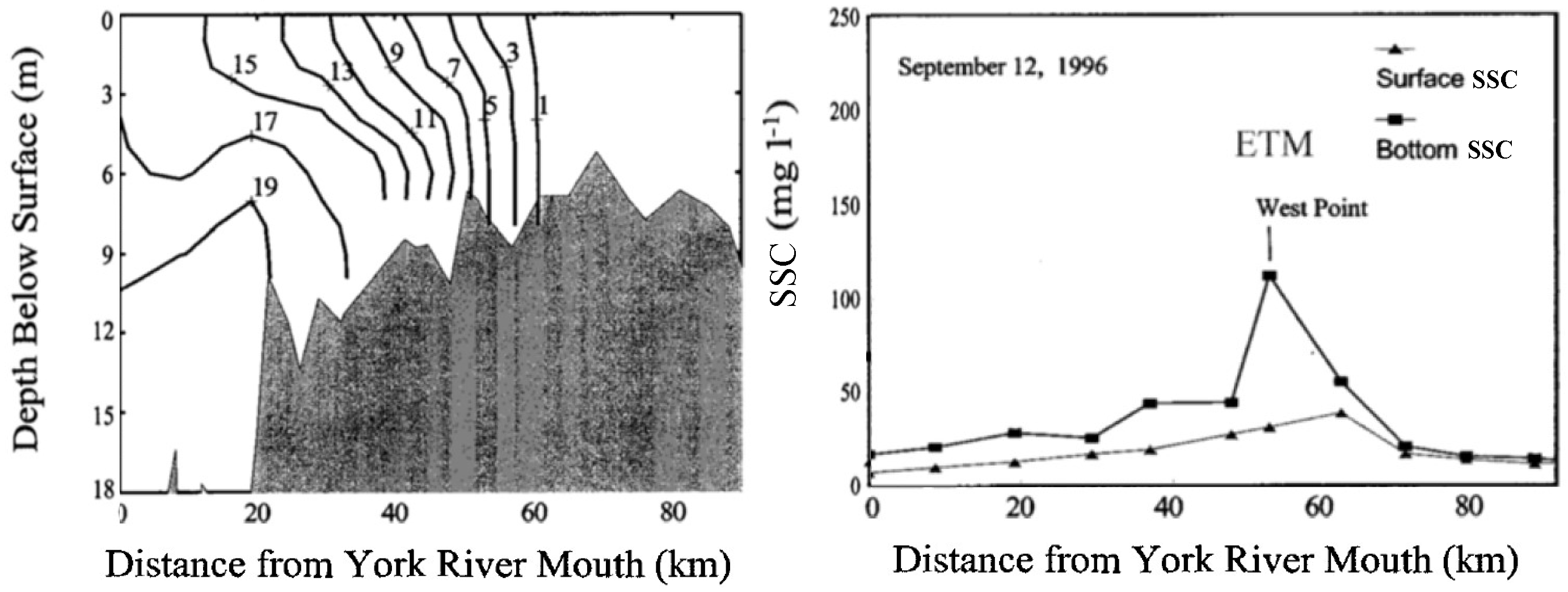
2.1. York River Estuary, Virginia, USA

The York River estuary [17], which inspired the idealized model geometry utilitzed in this study, extends northeast from the lower Chesapeake Bay (where salinities are typically ~26 g kg⁻¹) to the confluence of the Pamunkey and Mattaponi rivers, with a total length of ~60 km (Figure 1). The depths in the main channel range from ~20 m at the mouth to ~6 m at the head of salt (~1 g kg⁻¹ isohaline; Figure 2; [83]). The York is a microtidal, partially mixed estuary that becomes relatively more well-mixed as its depth decreases and tidal energy increases towards its head [83]. Under typical conditions, tidal current magnitude is on the order of 50 cm s⁻¹ at 1 meter above the bed (mab) in the ETM region [17]. The sediment bed in the main channel is dominated by mud with percentages often exceeding 80% [84]. Total suspended solids within the ETM of 250 mg L⁻¹ have been measured during slack at 1 mab [83]. For suspended flocs in the York that follow a fractial relationship in size and density distribution, [38] found the median values for the fractal dimension, primary particle size, and primary particle density to be 2.4, 1.7 microns, and 1900 kg m⁻³, respectively.

2.2. Model Description

Our implementation of COAWST used components of CSTMS [73] and hydrodynamics associated with ROMS [77,85]. Unlike most previous implementations of the CSTMS, ours utilized the flocculation dynamics module, the bed consolidation/swelling routine, and sediment–induced stratification. We neglected the impacts of sand (non-cohesive sediment) because the York River channel is dominantly mud [84]. The flocculation dynamics were represented by a set of differential equations based on population balance equations described in detail elsewhere [48,49,53]. These equations allow the exchange of sediment mass between the defined size classes, depending on the rate of turbulent shear and the sediment concentrations. Bed consolidation was accounted for by increasing the critical shear stress for erosion with depth into the sediment bed, with model parameters based on erosion experiments [60,65,86]. To implement this within the cohesive version of the CSTMS, the user must define initial and equilibrium profiles for critical shear stress for erosion. The effective instantaneous profile of the critical shear stress can be altered by erosion or deposition, but is then nudged toward the equilibrium profile to simulate consolidation or swelling [53,65]. The adjustment for sediment-induced stratification is computed as in [73].

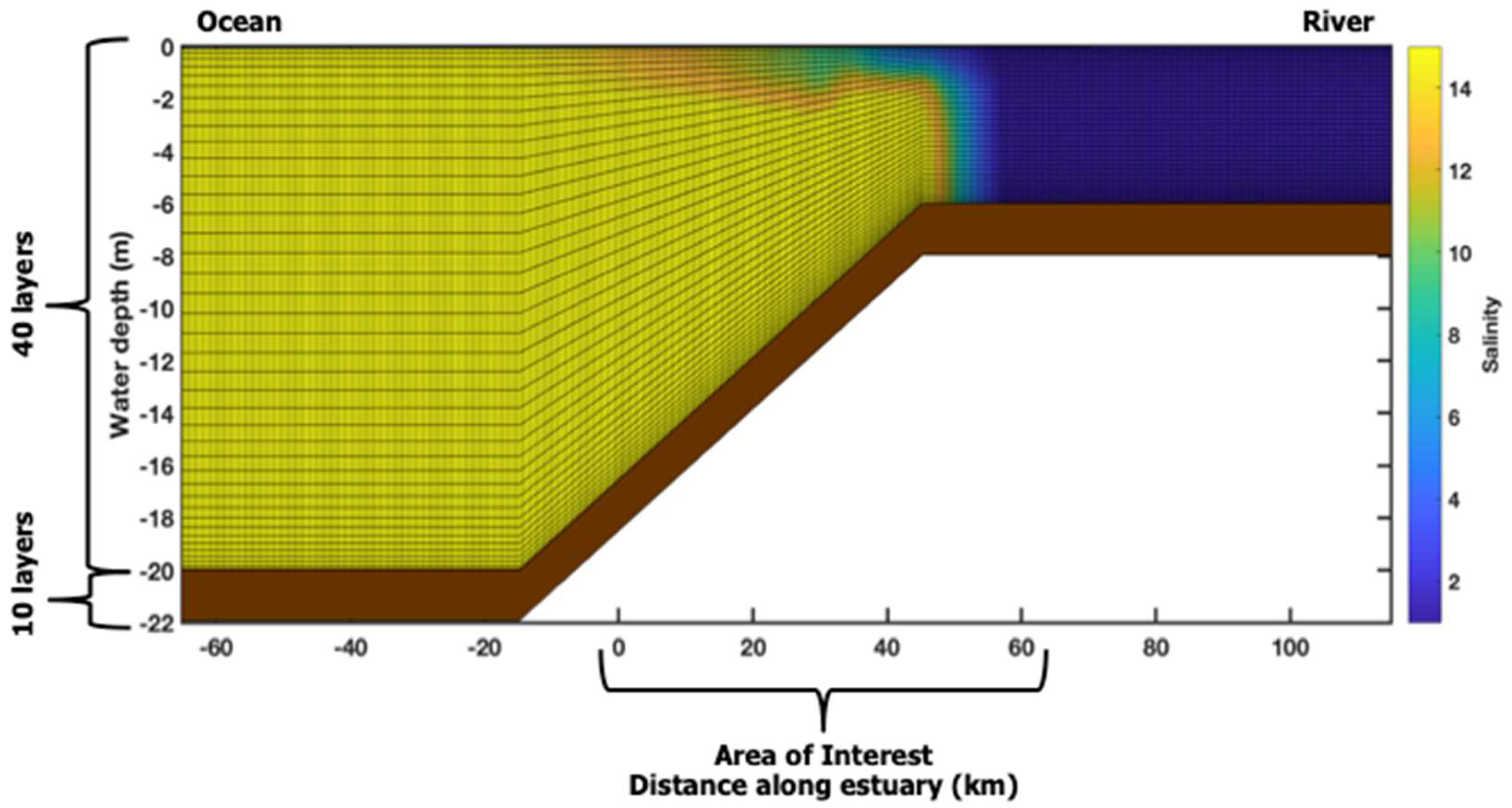
2.3. Model Configuration

A model with the following idealized two-dimensional domain was designed to represent the longitudinal dimension of a micro-tidal, partially mixed estuary. The model represented salinity-driven estuarine circulation, but neglected across-channel variation. The primary features of the idealized simulation were similar to the main channel of the York (see Section 2.1), and the sediment characteristics were based on observed values from this system [17,38]. The idealized estuary was 180 km in total length, and the water column was partitioned into 40 vertical layers (Figure 3). A 60–km-long area of interest was in the center of the grid, with a buffer of about 60 km on either end (please note that in the figures, “0 km” marks the seaward end of the area of interest). The horizontal resolution was 500 m, and the vertical resolution varied with depth and ranged from 0.053–0.79 m, with higher resolution near the surface and the bed. Our analysis focused on the area of interest that encompasses the estuarine system with water depths of ~18 m at the seaward end to the head of salt at the landward end with a depth of 6 m. The full model grid included buffer regions to either side, to minimize the effects of boundary conditions within the area of interest. The model applied includes salinity dependence for flocculation. A natural system is likely to have different floc properties in the riverine portion due to an absence of salinity. The “riverine” section of our domain lies within the upstream buffer zone, outside our region of interest.

The tides were driven at the ocean boundary with a period of 12 h and a micro-tidal range of 0.75 m at the mouth that increased to ~1 m at the head, as observed in the York River estuary [17], which produced tidal velocities similar to those observed in the York. The salinity at the seaward boundary was based on salinity measurements near the mouth of the York River estuary, which is open to the Chesapeake Bay. It was held constant in time, but varied in the vertical; specifically it was 26 psu near the bed and decreased to ~14 psu at the surface. Freshwater entered the grid at the upstream river boundary with a discharge of 70 m³ s⁻¹. On average, the salinity ranged between 0 and 25.5 psu in the area of interest. The temperature was held constant at 10 °C. The sediment model included 11 sediment floc size classes, with particle size diameters logarithmically spaced between 1 and 1024 μm, which represented the median diameter for each size class. These particle diameters span the range reported by [38]; from the inferred primary particle size through the largest flocs observed (~500 μm). We added an additional size class with a particle diameter of 1024 μm in order to account for larger flocs near the bed. The settling velocity (w_s,i) and density (ρ_f,i) of each class were calculated using a modified Stokes’ settling equation assuming a fractal dimension of 2.4, and a primary particle density and diameter of 2000 kg m⁻³ and 1 μm, respectively (based on observations from the York River estuary [38]; Equations (1) and (2);

Table 1. Sediment model size classes for floc diameters (D), along with corresponding floc density (ρ_f) and settling velocity (w_s). All eleven size classes were represented in the reference case and the sizes included in the reduced floc cases are indicated in columns 5 and 6.

i	D (μm)	ρf (kg m−3)	ws (mm s−1)	3 Class Case	5 Class Case
1	1	2000	0.00054	No	No
2	2	1663	0.0014	No	No
3	4	1441	0.0038	No	Yes
4	8	1294	0.0099	No	No
5	16	1198	0.026	Yes	Yes
6	32	1134	0.069	No	No
7	64	1092	0.18	No	Yes
8	128	1064	0.48	Yes	No
9	256	1046	1.27	No	Yes
10	512	1033	3.35	No	No
11	1024	1026	8.84	Yes	Yes

). For definitions of the variables in the equations below, see

Table A1. List and description of the variables and units used in equations.

Variable	Description
C	Total suspended sediment concentration (kg m−3)
Ci	Suspended sediment concentration for sediment class i (kg m−3)
D50	Median floc size (microns) by mass
Df,i	Diameter of the floc particle (m) for size class i
Dp	Diameter of the primary particle (m)
ρf,i	Density of the floc (kg m−3) for size class i
ρp	Density of primary particle (kg m−3)
ρw	Density of the water (kg m−3)
ρs	Density of quartz sediment (kg m−3)
G	Shear rate (s−1)
nf	Fractal dimension (non-dimensional)
N	Buoyancy frequency (s−1)
n	Grid layer number or cell number in x-direction
s	Sediment density divided by the water density
t	Time (s)
u	Flow velocity in x-direction (m s−1)
ν	Kinematic viscosity (m2 s−1)
ws,i	Settling velocity for sediment size class i (m s−1)
ws_mass	Mass settling velocity (m s−1)
x	Distance in the along estuary direction (m)
z	Distance in the vertical direction (m)

in the Appendix A.

$${\rho }_{f,i}={\rho }_w+\left({\rho }_p-{\rho }_w\right){\left(\frac{D_p}{D_{f,i}}\right)}^{3-n_f}$$

(1)

$$w_{s,i}=\frac{g\left({\rho }_{f,i}-{\rho }_w\right)D_{f,i}^2}{{\rho }_w · \upsilon }$$

(2)

In the equations above, ρ_w is the water density, ρ_p is the primary particle density, D_p is the primary particle diameter, D_f,i is the diameter of the floc in size class i, n_f is the fractal dimension, g is the acceleration due to gravity, and ν is the kinematic viscosity. No sediment was discharged from the river, and none left the domain through the river boundary, despite the gradient boundary condition.

Table 2. Open boundary conditions.

Process	River (East)	Ocean (West)
2D Momentum	Clamped	Flather
3D Momentum	Gradient	Gradient
Salinity/Temp	Clamped	Radiation/Nudging
Sediment	Gradient	Gradient
Free Surface	Gradient	Chapman Implicit

lists the open boundary conditions used. Other critical components to the sediment transport model included a logarithmic drag formulation with a constant hydraulic bottom roughness, for simplicity (z_0b = 5 × 10⁻⁵ m [45,75]), and we used the k-ε turbulence closure model [87]. The model setup was designed to approximately reproduce tidal fluctuations in velocity and SSC as observed in the York River estuary [17]. A time step of 30 s and the numerical schemes listed in

Table 3. Numerical schemes for the idealized estuary model.

Process	Numerical Scheme
Advection of momentum (Vertical, 3D)	4th order, centered
Advection of momentum (Horizontal, 3D)	3rd order, upstream
Advection of tracers	HSIMT 1
Vertical Sediment Settling	PPM 2

¹ Higher-order spatial interpolation at the middle temporal level [88]. ² Piecewise parabolic method [89].

were utilized.

2.4. Model Experiments

All model simulations presented here used the following procedure. The model was initialized with vertically homogenous salinity contours ranging from 0–26 evenly spaced surrounding the area of interest in the model domain (−22 to 65 km) and the water column was at rest (u = 0 m s⁻¹). The model was run for 90 days to allow the water column properties to adjust to the tidal conditions. The velocity and salinity fields output at the end of the 90-day run were used to initialize a 45-day run that included sediment transport and the routines for sediment-induced stratification, bed consolidation and swelling, and flocculation dynamics. In the 45-day run, the water column was initialized with no sediment in suspension, and the sediment bed was initialized with equal proportions by mass of all the floc size classes, with an initial critical shear stress of erosion profile based on data from the York River estuary taken in April 2006 following [45]. The final sediment bed characteristics, suspended sediment concentrations, velocity, and salinity fields from this 45-day run were then used as the initial conditions for a set of 30-day long case runs. Sediment was eroded from the bed in the same size class it was deposited for all runs that included flocculation dynamics. Additionally, when the bed consolidation routine was used, the consolidation timescale was 1 day, the swelling timescale was 100 days, and the equilibrium critical shear stress profile was based on data from the York River estuary taken in September 2006, also following [45]. Cases that neglected the bed consolidation routine used the default (non-cohesive) erosion formulation that calculates an active layer thickness [73].

Table 4. Sediment processes implemented in different model cases.

Case Name	Sed. Strat.	Consolidation	Flocculation	No. of Sed. Classes
Reference	Yes	Yes	Yes	11
No Floc.	Yes	Yes	No	11
No Strat.	No	Yes	Yes	11
No Consol.	Yes	No	Yes	11
3 classes	Yes	Yes	Yes	3
5 classes	Yes	Yes	Yes	5

lists the case runs, the cohesive processes incorporated into each, and is summarized here. The reference case run incorporated the three cohesive processes described above, i.e., flocculation, bed consolidation, and sediment–induced stratification. The along estuary velocity (u) and shear rates (G) were used to show changes in hydrodynamic conditions that would transport sediment or influence floc size. The SSC, the floc size distribution in suspension and the sediment bed, and weighted settling velocity by mass were used to evaluate sediment distributions and reasoning behind changes in sediment distributions. The weighted settling velocity by mass (w_{s_mass}) provided insight on how quickly sediment will settle based on the amount of each floc size that was in suspension. For the reference case, the median floc diameter (D₅₀) by mass was also compared to D₅₀ estimated by an equilibrium theory to examine the influence of SSC and shear rate on floc size.

The impact of individual cohesive processes on sediment distribution was then examined by completing additional case runs, each of which removed one of the processes from the implementation. The average depth-integrated suspended mass and average sediment size distribution from the case runs were used to assess changes in sediment distribution compared to the reference case. To evaluate the relative importance of flocculation and bed consolidation, the weighted settling velocity by mass and the average change in suspended masses for the case runs that neglected these processes were compared to estimates from the reference case. The gradient Richardson number was used to compare the suspended sediment impacts on density-induced stratification relative to salinity alone (Equations (3) and (4)).

Sensitivity to the number of sediment size classes was also evaluated. The number of sediment classes was reduced to five and three sizes from the eleven size classes in the reference case. The classes chosen for the test cases were selected in an attempt to maintain the size range while using fewer size classes. The run time, the depth averaged suspended sediment mass, the average size distribution, median size and mode, as well as the average mass weighted settling velocity were compared to reference case.

$$R{i}_{grad}={\left(\frac{N}{\raisebox{1ex}{$du$}\!\left/ \!\raisebox{-1ex}{$dz$}\right.}\right)}^2$$

(3)

$$N^2=-g\left(s-1\right)\frac{dC}{dz}-\frac{g}{{\rho }_w}\frac{\partial {\rho }_w}{\partial z}$$

(4)

In the equations above, N is the buoyancy frequency, u is the along estuary velocity, z is the depth, g is the acceleration due to gravity, s is sediment density divided by the water density, C is SSC, and ρ_w is the water density. Two Richardson numbers (Ri_grad) were calculated: one included the contribution of suspended sediment in the buoyancy frequency (N), and the other did not. See Table A1 in the Appendix A for a definition of symbols. For the version of the Ri_grad that neglected sediment–induced stratification, only the second term in Equation (4) was used in the calculation of N.

3. Results and Discussion

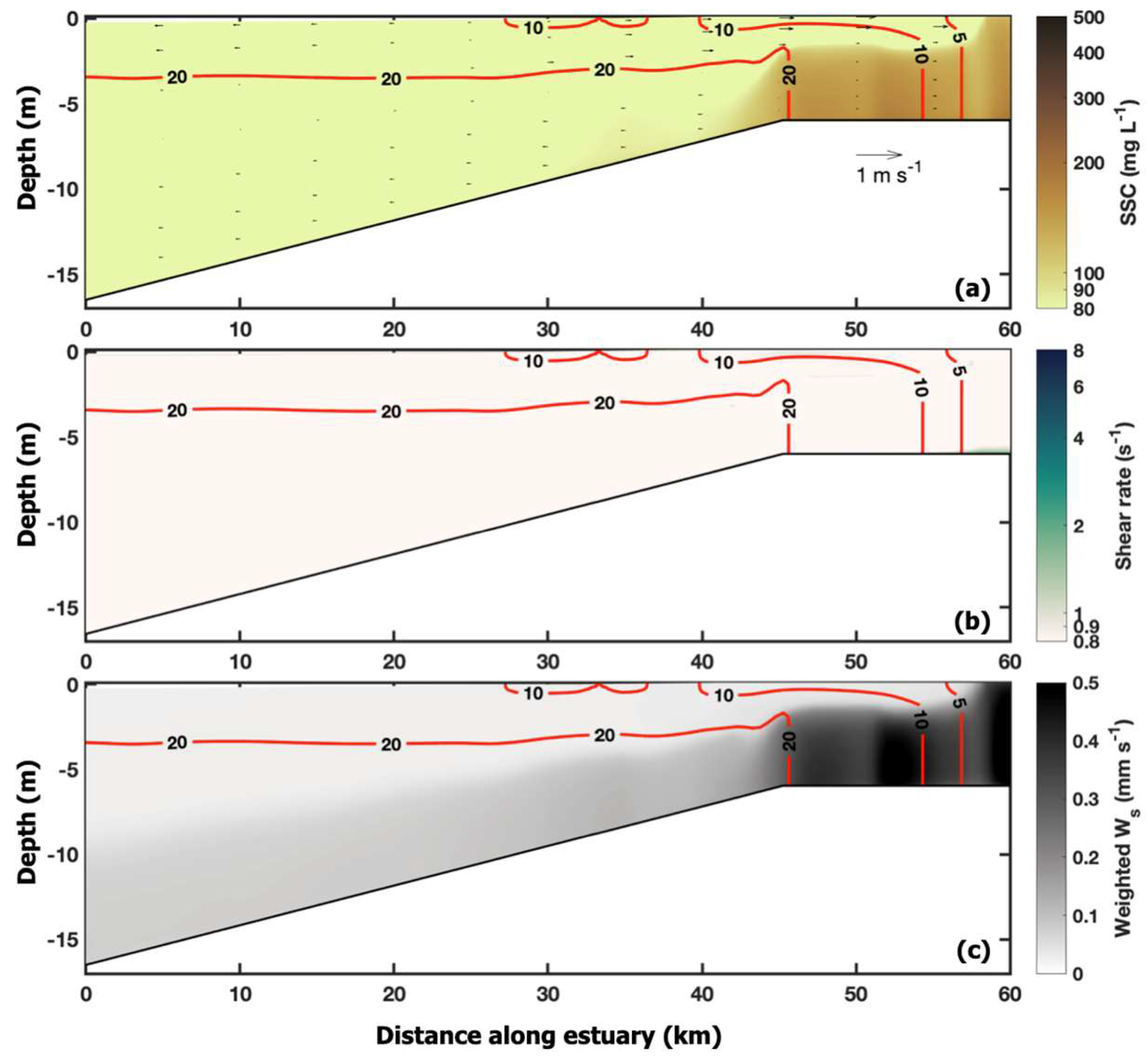
3.1. Reference Case

The reference case model that incorporated cohesive sediment processes (flocculation, bed consolidation, and suspended sediment stratification) showed distinct patterns in the suspension and transport patterns linked to changes in hydrodynamics along the estuary. Compared to other locations along the estuary, the up-river boundary of salt intrusion had the strongest vertical salinity gradient, and the near-bed, tidally averaged along-estuary currents converged at this location, as expected for a partially mixed estuary. Also, this convergence trapped and accumulated sediment in the region and created an Estuary Turbidity Maximum (ETM; Figure 4a and Figure 5a). Throughout the estuary, the suspended sediment concentration peaked near the bed and decreased with height above the bed (Figure 4a and Figure 5a). Several processes limited the diffusion of sediment into the upper water column, including reduced mixing across the halocline, and median floc sizes whose relatively fast settling velocities hindered their upward mixing. Shear rates were greatest near the bed and near the ETM region, especially during flood tide (Figure 4b and Figure 5b). At a height of 0.19 mab, maximum tidal shear reached 10 s⁻¹, which is comparable to the shear rate of 12 s⁻¹ for maximum tidal flow produced in the laboratory for a previous zero-dimensional application of FLOCMOD [49]. Looking at the lower half of the water column where both concentrations and shear were relatively high, the larger sizes formed by aggregation were found near the bed where there was enough shear to keep them in suspension. This was evident from a larger w_{s_mass} near the bed versus smaller settling velocities in the upper layers of the water column (Figure 4c and Figure 5c).

The bathymetric change in the upper estuary added some complexity but also relevant realism for this application relative to the CSTMS/COAWST model domains used by [87] and [53]. Specifically, the bathymetric step helped constrain the along-channel location of the maximum in tidal velocity and vertical mixing, along with the resulting salinity front and ETM, to be in the general vicinity of the transition from the deeper estuary to the shallower river, as seen in partially mixed estuaries such as the York, James, and Rappahannock ([17,90]). Nonetheless, the resulting SSC in the reference simulation was on the same order of magnitude and the ETM was roughly the same distance from the estuary mouth as the model results from [87]. The ETM in [53] typically occurred ~20 km from the mouth and SSC was up to 400 mg L⁻¹ higher than the concentrations shown here. These differences were not surprising, given that the present model used parameterizations chosen for the York River. Specifically, compared to [53], we used a larger fractal dimension, a smaller primary particle size, and lower floc particle densities. This study also used a different equilibrium critical shear stress for erosion, and longer consolidation and swelling timescales for the bed consolidation parameterization.

The median floc sizes, D₅₀, predicted from FLOCMOD within the ETM were interpreted in the context of an equilibrium floc size theory that postulates that a floc distribution at equilibrium will exhibit a linear relationship between D₅₀ and the ratio of SSC by mass (C) to the square root of the shear rate (G) [46,53]. To explore this with our model results, the ETM D₅₀ was calculated as the diameter at which 50% of the suspended flocs were smaller by mass and compared to C/G^1/2 (Figure 6). Hourly data for the last ten days of the model run were analyzed to avoid effects of model spin-up. Throughout much of the water column in the ETM, model results for periods with relatively high shear rates (i.e., between 4–12 s⁻¹) did indeed display a linear relationship between D₅₀ and C/G^1/2 consistent with an equilibrium floc distribution (Figure 6). Data from 0.70 mab and higher in the water column, during times with shear rates between 4 s⁻¹ and 12 s⁻¹, and SSC exceeding 100 mg L⁻¹ were used to fit an equilibrium line (inset in Figure 6). These conditions were assumed to be mostly likely at equilibrium.

At times when the model produced a D₅₀ that fell well above or below the equilibrium line in Figure 6, the modeled floc size was interpreted as larger or smaller than the equilibrium, which indicated that another process was likely influencing the size of the flocs in suspension. The median floc size in most of the water column alternated between lying near the predicted equilibrium size to being finer-grained than the equilibrium. In contrast, the model output that most consistently fell above the equilibrium line was for the very near-bed grid cell at 0.036 mab (triangles in Figure 6). These deviations from equilibrium were caused by non-local process such as settling from the upper water column and sediment input via seabed resuspension or advection; or local processes that lead to relatively long time scales for aggregation and disaggregation.

Next, we explored time-dependent variability within the ETM region for the reference case starting with the hydrodynamic and sediment conditions nearest the seafloor (0.036 mab). The tidal velocities reached around 40 cm s⁻¹ during peak flood, when the near-bed conditions for the shear rates were about 225 s⁻¹, and SSCs were ~800 mg L⁻¹ (Figure 7a–c). Both the peaks in the shear and SSC corresponded with the velocity maximum (Figure 7a–c) and the larger particles in suspension, with the very largest seen at peak flood (Figure 7d). An examination of floc size distributions (Figure 7d,g) revealed that during peak tidal flow, the median floc size, at ~190 μm, exceeded the equilibrium and there were larger floc sizes on the sediment bed surface as finer grains had been winnowed (Figure 7f). The flow velocity and shear was again elevated during ebb flow but remained less energetic than during flood. These currents were strong enough to erode sediment from the bed, and produced an ETM floc size distribution that included larger size classes as during flood flow, but were slightly smaller (not shown). The larger particles in the near-bed suspension during peak flows may be attributed in part to erosion of larger aggregates from the bed, as well as enhanced mixing and elevated SSC that promoted floc growth (Figure 7). However, during slack flow the near-bed D₅₀ equaled the equilibrium at ~70 μm (Figure 7g). As velocity decreased the larger, faster-settling floc sizes settled, leaving smaller sizes in suspension. Also, the sediment bed became enriched in the fractions of smaller floc sizes, as bed stresses decreased and the medium fractions could settle to the bed without being resuspended (Figure 7i). A two-dimensional idealized model utilizing the Chesapeake Bay ETM as a prototype predicted comparable near-bed SSC in the ETM of ~200 mg L⁻¹ near slack and 400 mg L^-1 during flood flow, and the median floc size during flood was ~150 μm, but the largest flocs were predicted during slack flow [91].

Higher in the water column (0.90 mab) at the ETM, the fluctuations in velocity were larger, but the shear and SSCs were smaller compared to near the bed (Figure 7a–c). The floc size distribution had a smaller concentration of the mid-sized sediment classes, which produced a larger D₅₀ than near the bed. Unlike the near-bed, D₅₀ at 0.90 mab equaled the predicted equilibrium D₅₀ of ~256 μm at peak flow (Figure 7e), and was smaller at ~90 μm than equilibrium at slack water (Figure 7h). At slack flow, the D₅₀ at 0.90 mab was similar to the value in the near-bed grid cell, as larger floc sizes had settled. The SSC at 0.90 mab was on average ~2 times smaller than at 0.036 mab (Figure 6c), whereas G^1/2 at 0.90 mab was ~7 times smaller than at 0.036 mab (Figure 7b). Thus, differences in C/G^1/2 and the equilibrium D₅₀ very near the bed versus higher in the water column were driven more by differences in shear rate than by differences in SSC. Overall, the ETM concentrations and floc sizes simulated in this study were smaller than those predicted at 0.80 mab in the idealized ETM model for the Chesapeake Bay [91].

The conditions in the lower reaches of the estuary differed from the ETM in that the tidal velocities, the square root of the shear, and SSC respectively stayed below 40 cm s⁻¹, ranged between 2–10 s^−1/2 and ranged between 50–90 mg L⁻¹ in the bottom 1.75 m (Figure 8a–c). These SSC values were similar to concentrations predicted in the downstream portion of an idealized estuary in [87]. The tidal fluctuation in velocity was greater at 1.75 mab than directly above the bed, but the shear rate showed greater tidal fluctuation and magnitude near the bed (Figure 8a,b). The SSC, the floc distribution, and D₅₀ showed minimal tidal variation in the bottom 1.75 m (Figure 8c–e,g,h). Near the bed (~0.078 mab), the floc size was equal or near the predicted equilibrium floc sizes both near slack and peak flood flow. Higher in the water column (1.75 mab), the modeled median diameters were smaller than the equilibrium floc sizes. The SSC to the square root of shear rate ratio was larger higher in the water column, leading to a larger predicted equilibrium floc size than was calculated by the time-dependent model. Case studies from [92] also showed situations where the floc size was over predicted by the [46] model. The floc size within the sediment bed downstream did not change over the tidal cycle (Figure 8i).

The results from the reference case demonstrate the variability of floc size under simplified tidal conditions, specifically within the ETM region. The results highlight that the assumption of an equilibrium floc size may not be valid here, because suspended floc sizes within the ETM often deviated from the equilibrium values. As also shown, the floc size predicted by the flocculation routine for the water column outside the ETM was fairly constant though it did not equal the equilibrium floc size. Therefore in the lower reaches of the estuary, a simulation with an appropriately chosen constant floc size and settling velocity could likely yield similar predictions of SSC as the present flocculation routine.

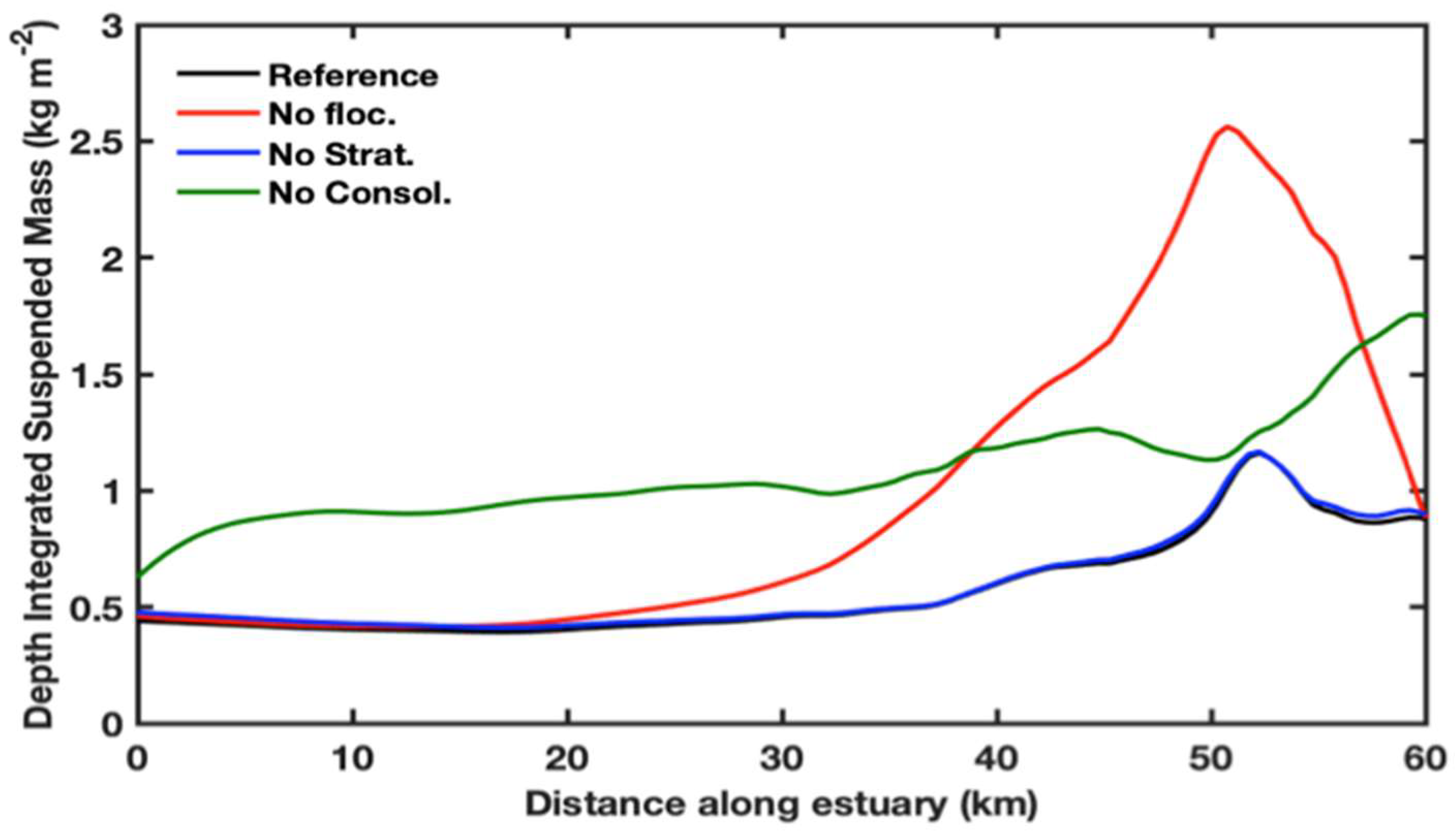
3.2. Sensitivity Tests

The impacts of flocculation, bed consolidation, and suspended sediment induced stratification to the distribution of sediment in the idealized estuary was further explored by comparing the results from the reference case to the test cases that neglected each of these processes (Table 4).

3.2.1. Impacts of Flocculation vs. No Flocculation

The role of flocculation was evaluated by comparing results from the reference case, which included flocculation to the “no floc” case (Table 4). Including flocculation dynamics shifted the size distribution of suspended matter to the larger size classes relative to the no flocculation case, as seen in the size distribution for the ETM (Figure 9a,b). The time-averaged D₅₀ by mass in the ETM size distribution increased to 123 μm with flocculation, compared to 55 μm in the no flocculation case. Overall, the effect of flocculation was most significant in the upstream portion of the estuary, where flocculation in the reference run decreased the depth-integrated suspended mass by ~2.5 times in the ETM, compared to the no flocculation run (Figure 10). The size of sediment in suspension increased even though flocculation reduced the SSC, producing a higher w_{s_mass} in the ETM relative to the no flocculation run (Figure 11a,b). Flocculation increased particle size and as a result increased the settling velocities of the suspended sediment in the ETM. This limited the transport of sediment out of the ETM, and increased deposition there.

For individual size classes, the difference in suspended mass between the reference and no flocculation cases showed that in the ETM (found at ~45–55 km), flocculation moved mass from the smaller size classes ≤64 μm into larger classes ≥256 μm (Figure 12). In the lower estuary (≤~30 km), including flocculation generally removed mass from the smallest size classes of 1–16 μm in diameter (blue in Figure 12a,b); but increased suspended mass in the median sizes (red in Figure 12c,d). These larger particles with higher settling velocities concentrated closer to the bed, so that flocculation reduced SSC in the surface waters of the lower estuary (Figure 12).

3.2.2. Impacts of Bed Consolidation vs. No Consolidation

The time-averaged size distribution from the ETM when bed consolidation was included showed the D₅₀ by mass was reduced to 123 μm, compared to 170 μm when bed consolidation was neglected (Figure 9c). The depth-integrated suspended mass was reduced throughout most of the estuary; ETM concentrations were ~1.5 times smaller in the reference case than those calculated in the no consolidation case (Figure 10). The settling velocities (w_{s_mass}) were lower when bed consolidation was included compared to the case that neglected bed consolidation (Figure 11a,c). The reference run with consolidation showed that relative to no consolidation, suspended mass was removed from the larger size classes (128–1024 μm), and suspended mass was added to the smaller sizes in most of the estuary (Figure 13). Throughout the area of interest, bed consolidation reduced bed erosion, lowering the SSC and the probability of flocculation to occur, which shifted the size distribution to smaller sizes compared to the no consolidation case (Figure 13).

3.2.3. Impacts of Sediment-Induced Stratification

Density-induced stratification due to gradients in SSC did not significantly impact sediment patterns; the size distribution of suspended sediment was similar to the distribution calculated when sediment-induced stratification was removed, the time averaged D₅₀ was 123 μm for the reference case compared to 116 μm for the case that neglected sediment-induced stratification (Figure 9d). The depth-integrated suspended sediment mass throughout the estuary for the reference case was nearly identical to the no stratification case (Figure 10). These results indicate that the SSC gradients estimated in this set of model runs were not sufficient to induce significant stratification. The gradient Richardson number (Ri_grad; Equations (3) and (4); [93]) was calculated for 0.5 and 1.0 mab throughout the area of interest. Suspended sediment on average contributed minimally to the Ri_grad. When the Ri_grad exceeded the critical value of 0.25, SSC contributed 2.5% to the Ri_grad at 0.5 mab, and 1.8% at 1 mab. Please note that the density of the flocs decreased with size, as was observed in the York River estuary (Table 1; [38]). Suspended sediment-induced stratification could be more important in situations where the density of large flocs did not decrease, where higher stresses or higher erodibility led to higher SSC near the bed, or where stronger temperature/salinity stratification more significantly enhanced sediment-induced stratification.

To summarize Section 3.2.1, Section 3.2.2, Section 3.2.3, flocculation dynamics were especially important in the ETM, while bed consolidation impacted suspended sediment throughout the estuary. Based on these results, future modeling studies in cohesive environments should consider using flocculation if variability in SSC and shear rate is comparable or stronger than the ETM modeled here. However, changes in erodibility due to consolidation is important for most studies in regions with muddy or mixed-sediment beds. For this implementation, density-induced stratification due to SSC gradients was less important for suspended sediment dynamics. The SSCs in this study were <1000 mg L⁻¹ and floc densities were ≤2000 kg m⁻³; thus sediment-induced stratification could be neglected in studies with similar sediment dynamics. However, if a user is unsure, it is best to incorporate density-induced stratification from sediment, as this routine has a low computational cost in COAWST and may impact sediment distributions and mixing.

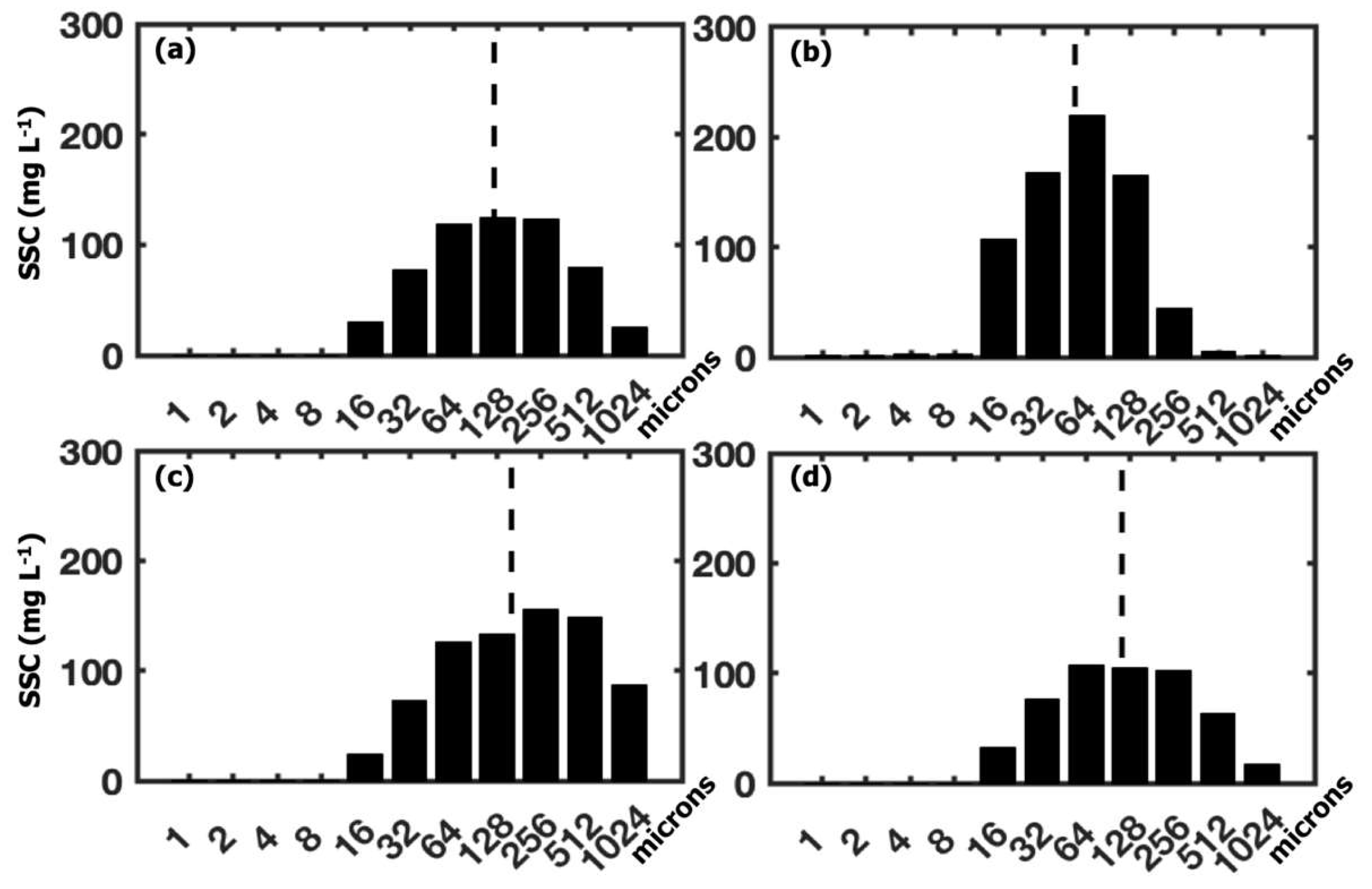
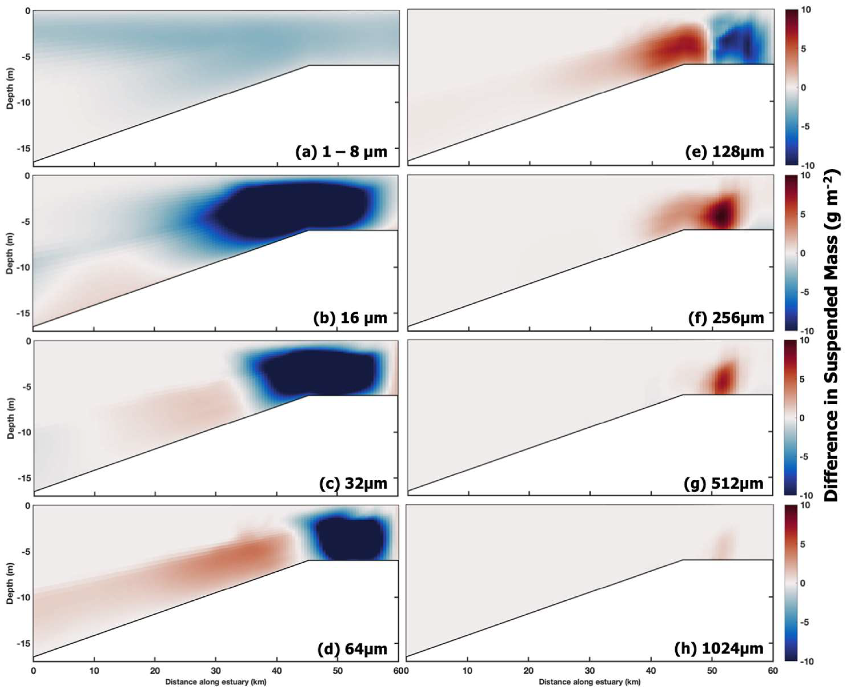
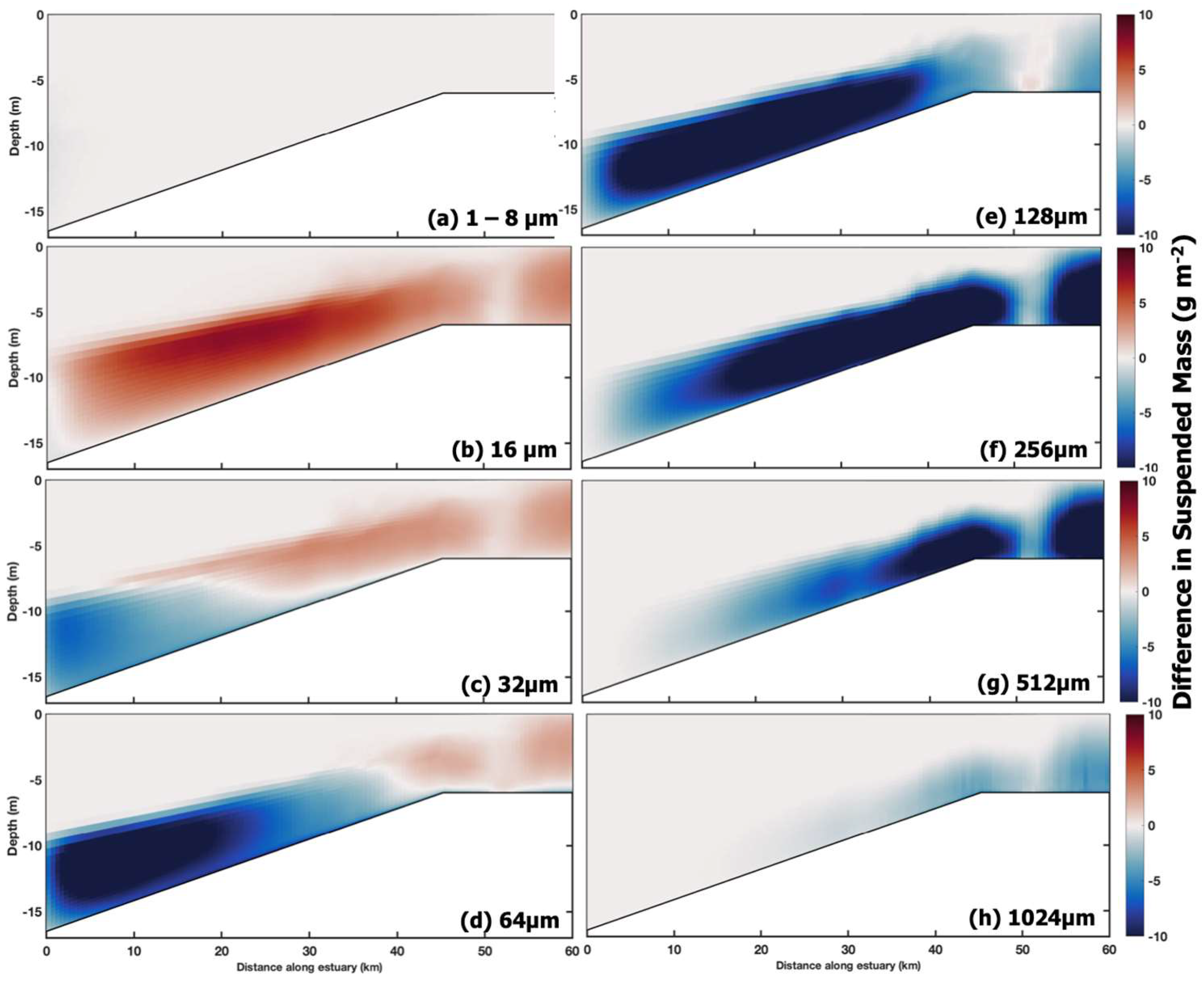
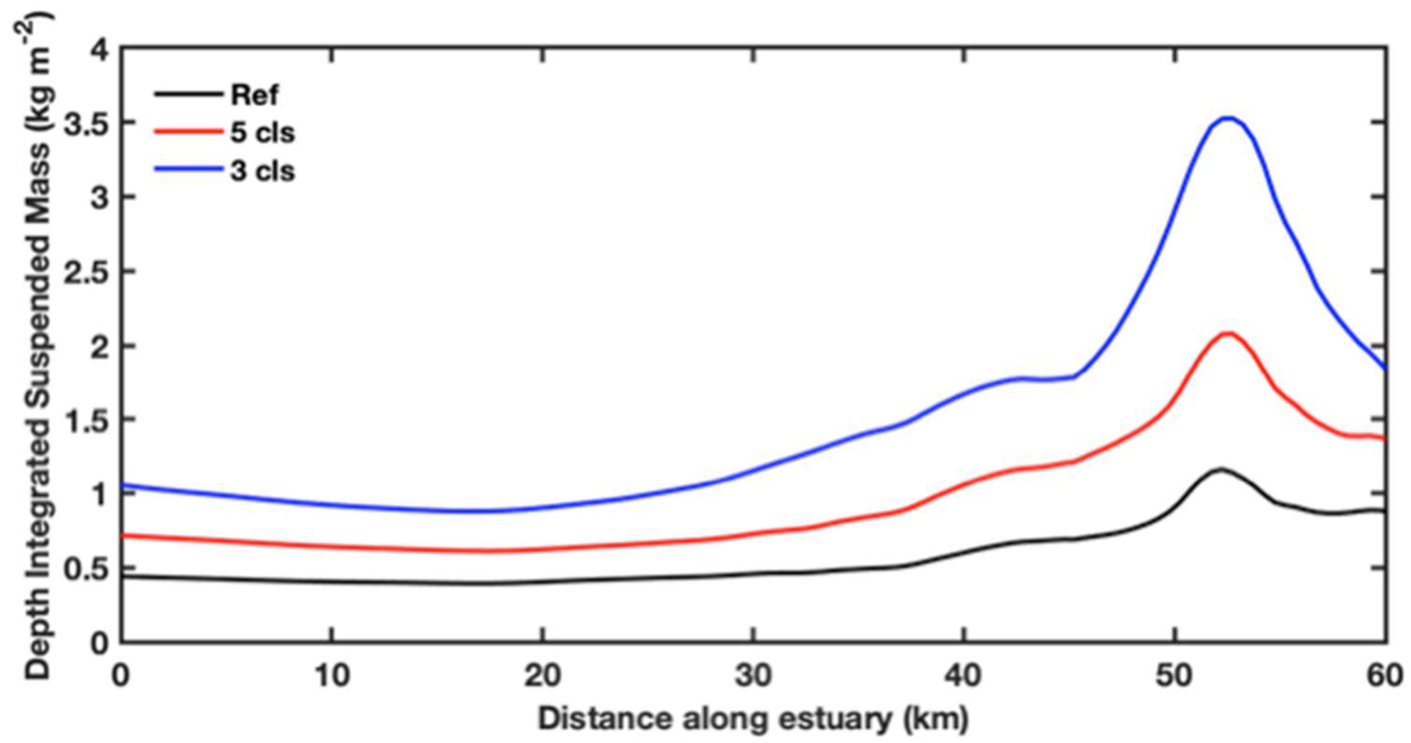
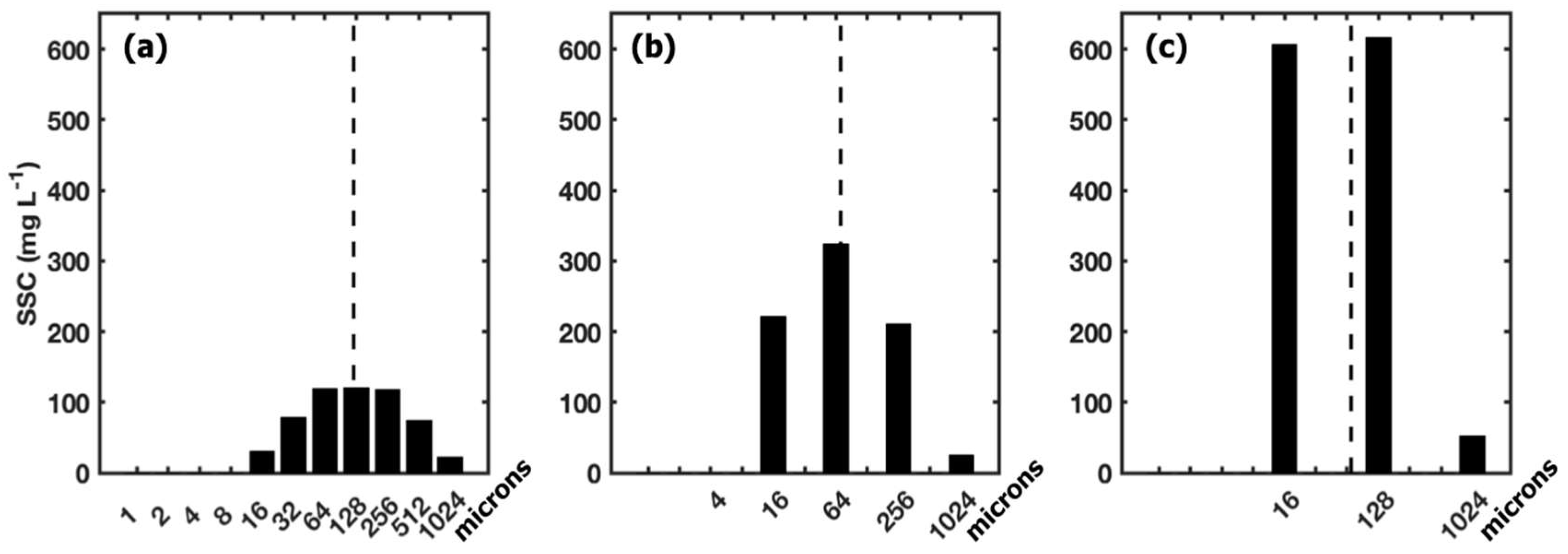
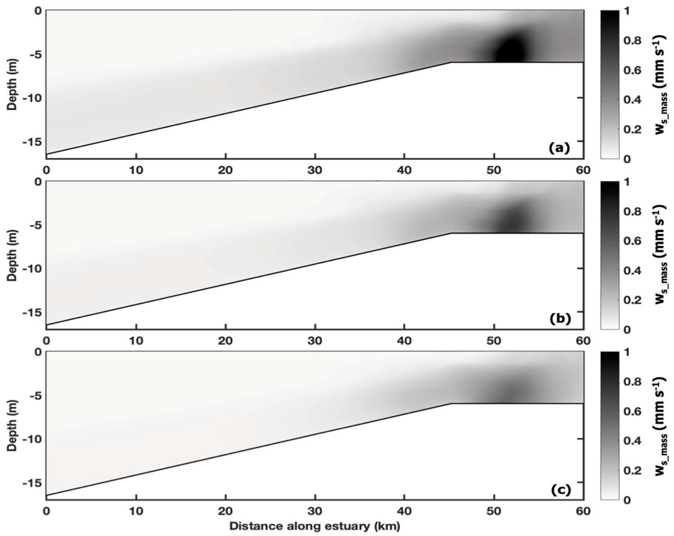
3.2.4. Sensitivity to the Floc Size Distribution

The final set of cases evaluated the sensitivity of model estimates to the number of size classes used to represent the floc population. Results showed that the calculations of SSC were sensitive to the number of size classes used. Reducing the number of sediment sizes from eleven classes in the reference case to five or three increased the amount of suspended sediment throughout most of the estuary (Figure 14). The case using only three size classes produced depth-integrated suspended sediment that exceeded those from the case that neglected flocculation; the peak concentration in the three size class case was approximately 30% higher than the no flocculation case (Figure 14).

The modal and D₅₀ floc size in suspension by mass were sensitive to the resolution of the floc size distribution. When five size classes were used, suspended mass near the bed in the ETM had a modal size of 64 μm, whereas the reference run had a modal size diameter of 128 μm (Figure 15a,b). The D₅₀ by mass of the five-size class run was 74 μm compared to the reference case D₅₀ of 123 μm. For the three-size class run, the floc D₅₀ near the bed in the ETM was similar to the 5-size class run at 72 μm. However, the modal size was similar to the reference case at 128 μm, but there was much more suspended mass for the three-class case compared to the reference case (Figure 15). The changes to suspended size distribution likewise reduced the weighted setting velocities calculated for the three and five class cases, compared to the reference case (Figure 16). The case with only three size classes had the smallest w_{s_mass} of the cases considered (Figure 16c).

The computational expense of the flocculation module was related to the number of size classes used. The maximum number of size classes used in this study was eleven because the computational expense to use more was prohibitive. Including flocculation dynamics in the reference model that had eleven sediment classes increased the computational time by a factor of ~130 (run time of ~128 h with flocculation and ~1 h without). Using five or three size classes increased the cost by factors of ~31, and ~13.4, respectively, compared to not using flocculation dynamics. Finding the optimal set of floc sizes may take several test runs to determine the best configuration as shown in previous studies [49]. Size distributions from our test cases indicated that representing the particles that are abundantly found in suspension (i.e., sizes 16–512 μm in our idealized estuary) is more important than maintaining the complete possible size range. This set of sensitivity shows that to apply the flocculation model in other environments, using a one- or two-dimensional domain would be useful for designing an appropriate floc distribution and optimal number of sediment classes to represent. Additionally, the availability of observation-based detailed information on the floc size distribution is important for designing the size distributions for FLOCMOD. The flocculation routine was found to be sensitive to the characteristics assigned to size classes, therefore care should be taken in assigning floc properties. For these reasons, it remains challenging to select an optimal size distribution and associated sediment characteristics of sediment size classes that optimize the results while limiting computational costs.

4. Key Implications and Future Directions

The case presented in this study showed that sediment size distributions vary along a representative muddy, partially mixed estuary. Our results showed that the processes of bed consolidation and flocculation modified the sediment erodibility and settling velocity within the idealized estuary over tidal timescales. However, many sediment transport models hold these sediment characteristics constant when modeling an entire estuarine system, which can lead to under- or overestimates of SSC. The cohesive process sensitivity tests indicated that it was important to include bed consolidation in estimating the SSC along the estuary. Flocculation was important in areas of the estuary with tidal variability, that has a range similar to or greater than 300 mg L⁻¹ and 8 s⁻¹ in SSC and shear rate, respectively, as was the case for 0.90 mab in the ETM of this idealized estuary. However, due to the sensitivity of the flocculation routine to the size class distribution and other sediment characteristics, observational data are still needed to appropriately constrain the resulting SSC. Additional modeling studies are warranted to help determine the optimal sediment parameters for FLOCMOD. Since the flocculation routine is computationally expensive, a set of one-dimensional runs that more systematically vary the sediment size classes and properties may be useful for parameterizing FLOCMOD for natural estuaries.

There are motivations for using FLOCMOD in regional scale domains despite the computational expense. Employing FLOCMOD in regional studies is now relatively straightforward, because the module has been coupled with the CSTMS [53]. The population balance equations fit well within the CSTMS piecewise parabolic settling scheme [73], chosen to reduce limitations by the CFL (Courant Friedrichs Lewy) stability criteria. Coupling less computationally expensive flocculation routines, such as those that track changes in effective floc settling velocity [46,94], would require structural change to the vertical advection scheme used within the CSTMS, which assumes that the settling velocity of each particle class remains constant throughout the water column.

One approach to assessing the impact of flocculation for a location while maintaining a modest computational expense is to apply FLOCMOD within a small one-dimensional vertical domain, with realistic physics and bed dynamics. This could be a reasonable method for evaluating flocculation dynamics for an area of interest such as the York River estuary ETM. In the York River estuary, flocculation dynamics seem more important within regions with elevated SSC, compared to the rest of the estuary. Further work on reducing the computational cost of the flocculation routine by reducing the number of vertical water column layers, or modifying the FLOCMOD convergence criteria, could make a three-dimension model more cost effective and provide added insight on the distribution of flocs under more realistic and complex bathymetric conditions.

The flocculation formulation may also be useful for examining the formation, dispersal, and fate of oil-mineral aggregates. Parameterization of FLOCMOD could be modified to represent the properties of oil-mineral aggregates using data from laboratory experiments. For example, the growth and breakup parameters in Equations (7)–(12) from [49] may be modified to account for hydrocarbon content. This would allow the sediment transport routines within the CSTMS to be used to examine the dispersal of oil from a spill. However, this does not account for the impact of the bacterial communities that are attracted to oil–mineral aggregates and breakdown the oil, and excrete exopolymeric substances (EPS; [95]), which potentially changes the characteristics of the settling aggregates. Linking FLOCMOD to the HydroBioSed CSTMS module that has been used to account for biogeochemistry [96] may provide an avenue for incorporating microbial degradation with the flocculation process. This would be useful for tracking the formation, transformation, and transport of oil–mineral aggregates.

5. Conclusions

The idealized model developed in this study reproduced the key physical features of an estuary such as estuarine circulation and the formation of an ETM through flow convergence and sediment trapping. The flocculation model adequately represented the dynamics throughout the entire estuary, and the results demonstrated that sediment conditions in the ETM were more variable over the tidal cycle with SSC ~3–10 times greater and median diameters ~2–8.5 times larger than downstream. In the ETM, the distribution of floc sizes fluctuated with the shear rate and SSC; the largest flocs in suspension were seen during flood tide, and these tended to deposit to the bed during slack flow. An equilibrium floc theory was applied to the modeled conditions that were assumed to be near-equilibrium (ETM, above the bed, and peak flow conditions) to derive a relationship between equilibrium floc diameter, SSC, and the shear rate. The analysis indicated much of the estuary was not at equilibrium but that other processes were impacting the floc size over much of the tidal cycle throughout the estuary. Additional analysis is needed to determine which other processes are influencing floc size and at which stage of the tidal cycle and where in the estuary are these other processes more dominate.

The impact of individual processes and user-defined floc size characteristics were evaluated through a series of case studies that individually excluded bed consolidation, flocculation, or sediment-induced stratification, and varied the number of floc sizes used. Flocculation dynamics had the largest impact on SSC within the ETM region where both suspended sediment and turbulence varied in time and space. Flocculation reduced the average depth-integrated suspended mass by ~50% within the ETM. Outside of the ETM, bed consolidation had the largest impact and similarly decreased the average depth-integrated suspended mass by ~50%. Sediment-induced density stratification had a much smaller impact on the distribution of sediment than either flocculation or bed consolidation. The vertical gradients in the suspended concentrations within the idealized estuary did not inhibit mixing based on the SSC contributions to the gradient Richardson number. The use of fewer size classes, to reduce computational expense, resulted in estimates of sediment concentration that increased by as much as ~3.5 times, and an estimated median floc size that decreased by as much as ~1.7 times relative to the reference case. The flocculation routine was sensitive to the number of floc size classes used and is also expected to be sensitive to the characteristics (i.e., settling velocity, critical shear stress) assumed for the floc classes.

The reference run in this study, though it represented an idealized estuarine configuration, was parameterized using observational data from the York River estuary. Other applications of the cohesive sediment model for a different location would require some insight into how to effectively parameterize these routines. The use of both observed SSCs and floc sizes helped us to constrain model parameters because multiple possible model configurations can yield similar SSC. Measurements of the suspended sediment size distribution based on in situ camera systems, laser instruments, and/or laboratory experiments can be especially useful for constraining fractal dimension and primary particle size and density [25,38,40,97,98,99]. Erodibility estimates obtained under variable environmental conditions, either through erosion experiments or calibrated estimates from a high sample frequency acoustic instrument [60,100] can provide constraints for the bed consolidation parameters.

Our study showed that sediment transport calculations in partially mixed, muddy estuaries may be equally sensitive to incorporating flocculation and bed consolidation. However, the inclusion of flocculation using a population-based floc model added significantly to the computational cost of our coupled sediment transport–hydrodynamic model. This may prove challenging for applying the population-based flocculation model to a regional-scale model domain, but the aggregation and disaggregation processes significantly impacted suspended sediment concentrations, and suspended grain size distribution.

References

1. Bianchi, T.S. Estuaries: Where the river meets the sea. Nat. Educ. Knowl. 2013, 4, 1–6. [Google Scholar]
2. Boyd, R.; Dalrymple, R.; Zaitlin, B.A. Classification of clastic coastal depositional environments. Sediment. Geol. 1992, 80, 139–150. [Google Scholar] [CrossRef]
3. Pritchard, D.W. Estuarine Hydrography. Adv. Geophys. 1952, 1, 243–280. [Google Scholar] [CrossRef]
4. Geyer, W.R.; MacCready, P. The Estuarine Circulation. Annu. Rev. Fluid Mech. 2013, 46, 175–197. [Google Scholar] [CrossRef]
5. MacCready, P.; Geyer, W.R. Advances in Estuarine Physics. Annu. Rev. Mar. Sci. 2010, 2, 35–58. [Google Scholar] [CrossRef] [PubMed] [Green Version]
6. Dyer, K.R. Sediment Processes in Estuaries: Future Research Requirements. J. Geophys. Res. 1989, 94, 14327–14339. [Google Scholar] [CrossRef]
7. Moore, K.A. Submerged Aquatic Vegetation of the York River. J. Coast. Res. 2009, 10057, 50–58. [Google Scholar] [CrossRef]
8. McSweeney, J.M.; Chant, R.J.; Wilkin, J.L.; Sommerfield, C.K. Suspended-Sediment Impacts on Light-Limited Productivity in the Delaware Estuary. Estuaries and Coasts 2017, 40, 977–993. [Google Scholar] [CrossRef]
9. Dalrymple, R.W.; Zaitlin, B.A.; Boyd, R. Estuarine Facies Models: Conceptual Basis and Stratigraphic Implications. J. Sedimentary Res. 1992, 62, 1130–1146. [Google Scholar] [CrossRef]
10. Dam, G.; van der Wegen, M.; Labeur, R.J.; Roelvink, D. Modeling centuries of estuarine morphodynamics in the Western Scheldt estuary. Geophys. Res. Lett. 2016, 43, 3839–3847. [Google Scholar] [CrossRef] [Green Version]
11. Nittrouer, J.A.; Best, J.L.; Brantley, C.; Cash, R.W.; Czapiga, M.; Kumar, P.; Parker, G. Mitigating land loss in coastal Louisiana by controlled diversion of Mississippi River sand. Nature Geosci. 2012, 5, 534–537. [Google Scholar] [CrossRef]
12. Nittrouer, J.A.; Viparelli, E. Sand as a stable and sustainable resource for nourishing the Mississippi River delta. Nature Geosci. 2014, 7, 350–354. [Google Scholar] [CrossRef]
13. Joshi, S.; Xu, Y.J. Assessment of Suspended Sand Availability under Different Flow Conditions of the Lowermost Mississippi River at Tarbert Landing during 1973–2013. Water 2015, 7, 7022–7044. [Google Scholar] [CrossRef]
14. Blanton, B.O.; Aretxabaleta, A.; Werner, F.E.; Seim, H.E. Monthly climatology of the continental shelf waters of the South Atlantic Bight. J. Geophys. Res. 2003, 108, 3264–3583. [Google Scholar] [CrossRef]
15. Blake, A.C.; Kineke, G.C.; Milligan, T.G.; Alexander, C.R. Sediment Trapping and Transport in the ACE Basin, South Carolina. Estuaries 2001, 24, 721–733. [Google Scholar] [CrossRef]
16. Nichols, M.M.; Johnson, G.H.; Peebles, P.C. Modern Sediment and Facies Model for a Microtidal Coastal Plain Estuary, The James River Estuary, Virginia. J. Sedimentary Res. 1991, 61, 883–899. [Google Scholar]
17. Friedrichs, C.T. York River physical oceanography and sediment transport. J. Coastal Res. 2009, 10057, 17–22. [Google Scholar] [CrossRef]
18. Nichols, M.M.; Poor, G. Sediment Transport in a Coastal Plain Estuary. J. Waterways Harbors Division 1967, 93, 83–95. [Google Scholar]
19. Cornwell, J.C.; Owens, M.S.; Boynton, W.R.; Harris, L.A. Sediment-Water Nitrogen Eschange along the otomac River Estuarine Salinity Gradient. J. Coastal. Res. 2016, 32, 776–787. [Google Scholar] [CrossRef]
20. Geyer, W.R.; Woodruff, J.D.; Traykovski, P. Sediment Transport and Trapping in the Hudson River Estuary. Estuaries 2001, 24, 670–679. [Google Scholar] [CrossRef]
21. Feng, H.; Cochran, J.K.; Lwiza, H.; Brownawell, B.J.; Hirschberg, D.J. Distribution of heavy metal and PCB contaminants in the sediments of an urban estuary: The Hudson River. Mar. Environ. Res. 1998, 45, 69–88. [Google Scholar] [CrossRef]
22. Bandara, U.C.; Yapa, P.D.; Xie, H. Fate and transport of oil in sediment laden marine waters. J. Hydro-Environment Res. 2011, 5, 145–156. [Google Scholar] [CrossRef]
23. Daly, K.L.; Passow, U.; Chanton, J.; Hollander, D. Assessing the impacts of oil-associated marine snow formation and sedimentation during and after the Deepwater Horizon oil spill. Anthropocene 2016, 13, 18–33. [Google Scholar] [CrossRef] [Green Version]
24. Burban, P.; Lick, W.; Lick, J. The Flocculation of Fine-Grained Sediments in Estuarine Waters. J. Geophys. Res. 1989, 94, 8323–8330. [Google Scholar] [CrossRef]
25. Smith, S.J.; Friedrichs, C.T. Size and settling velocities of cohesive flocs and suspended sediment aggregates in a trailing suction hopper dredge plume. Cont. Shelf Res. 2011, 31, S50–S63. [Google Scholar] [CrossRef]
26. De Jonge, V.N.; Schuttelaars, H.M.; van Beusekom, J.E.E.; Talke, S.A.; de Swart, H.E. The influence of channel deepening on estuarine turbidity levels anddynamics, as exemplified by the Ems estuary. Estuar. Coast. Shelf Sci. 2014, 139, 46–59. [Google Scholar] [CrossRef]
27. NOAA. What Percentage of the American Population Lives near the Coast? NOAA Ocean Services. Available online: https://oceanservice.noaa.gov/facts/population.html (accessed on 26 August 2019).
28. Chesapeake Bay Program. Strategies for Financing Chesapeake Bay Restoration in Virginia. Environmental Finance Center at the University of Maryland, 2017. Available online: https://www.chesapeakebay.net/documents/Strategies_for_Financing_Ches_Bay_Restoration_in_VA_FINAL_9.26.17.pdf (accessed on 12 September 2019).
29. Jantz, C.A.; Goetz, S.J.; Shelley, M.K. Using the SLEUTH urban growth model to simulate the impacts of future policy scenarios on urban land use in the Baltimore-Washington metropolitan area. Environ. Plan. B Plan. Des. 2004, 31, 251–271. [Google Scholar] [CrossRef]
30. Goetz, S.J.; Jantz, C.A.; Prince, S.D.; Smith, A.J.; Varlyguin, D.; Wright, R.K. Integrated Analysis of Ecosystem Interactions with Land Use Change: The Chesapeake Bay Watershed. Ecosyst. L. Use Chang. 2004, 153, 263–275. [Google Scholar] [CrossRef]
31. Shenk, G.W.; Linker, L.C. Development and application of the 2010 Chesapeake Bay Watershed total maximum daily load model. J. Am. Water Resour. Assoc. 2013, 49, 1042–1056. [Google Scholar] [CrossRef]
32. Irby, I.D.; Friedrichs, M.A.M.; Da, F.; Hinson, K.E. The competing impacts of climate change and nutrient reductions on dissolved oxygen in Chesapeake Bay. Biogeosciences 2018, 15, 2649–2668. [Google Scholar] [CrossRef] [Green Version]
33. Moriarty, J.M.; Friedrichs, M.A.M. Impact of seabed resuspension on oxygen and nitrogen dynamics in the northern Gulf of Mexico: A numerical modeling study. J. Geophys. Res. Oceans 2018, 123, 7237–7263. [Google Scholar] [CrossRef]
34. Irby, I.D.; Friedrichs, M.A.M.; Friedrichs, C.T.; Bever, A.J.; Hood, R.R.; Lanerolle, L.W.J.; Li, M.; Linker, L.; Scully, M.E.; Sellner, K.; et al. Challenges associated with modeling low-oxygen waters in Chesapeake Bay: A multiple model comparison. Biogeosciences 2016, 13, 2011–2028. [Google Scholar] [CrossRef]
35. Irby, I.D.; Friedrichs, M.A.M. Evaluating confidence in the impact of regulatory nutrient reduction on Chesapeake Bay water quality. Estuaries Coasts 2017, 42, 16–32. [Google Scholar] [CrossRef]
36. Droppo, I.G. Rethinking what constitutes suspended sediment. Hydrol. Process. 2001, 15, 1551–1564. [Google Scholar] [CrossRef]
37. Droppo, I.G. Structural controls on floc strength and transport. Can. J. Civ. Eng. 2004, 31, 569–578. [Google Scholar] [CrossRef]
38. Fall, K.; Friedrichs, C.; Massey, G.; Bowers, D.; Smith, J. Fractal Floc Properties in Estuarine Surface Waters: Insights from Video Settling, LISST, and Pump Sampling. 2019. Report, Virginia Institute of Marine Science Report CHSD-2019-01. Available online: http://www.vims.edu/chsd (accessed on 26 August 2019).
39. Milligan, T.G.; Hill, P.S. A laboratory assessment of the relative importance of turbulence, particle composition, and concentration in limiting maximal floc size and settling behaviour. J. Sea Res. 1998, 39, 227–241. [Google Scholar] [CrossRef] [Green Version]
40. Manning, A.J.; Bass, S.J.; Dyer, K.R. Floc properties in the turbidity maximum of a mesotidal estuary during neap and spring tidal conditions. Mar. Geol. 2006, 235, 193–211. [Google Scholar] [CrossRef]
41. Maggi, F. The settling velocity of mineral, biomineral, and biological particles and aggregates in water. J. Geophys. Res. Oceans 2013, 118, 2118–2132. [Google Scholar] [CrossRef]
42. Manning, A.J.; Spearman, J.R.; Whitehouse, R.J.; Pidduck, E.L.; Baugh, J.V.; Spencer, K.L. Flocculation Dynamics of Mud:Sand Mixed Suspensions. In Sediment Transport Processes and Their Modeling Applications; IntechOpen: London, UK, 2013; pp. 119–164. [Google Scholar]
43. Hill, P.S.; McCave, I.N. Suspended particle transport in benthic boundary layers. In The Benthic Boundary Layer: Transport Processes and Biogeochemistry; Oxford University Press: Oxford, UK, 2001; pp. 78–103. [Google Scholar]
44. Moriarty, J.; Harris, C.; Hadfield, M. A Hydrodynamic and Sediment Transport Model for the Waipaoa Shelf, New Zealand: Sensitivity of Fluxes to Spatially-Varying Erodibility and Model Nesting. J. Mar. Sci. Eng. 2014, 2, 336–369. [Google Scholar] [CrossRef] [Green Version]
45. Fall, K.A.; Harris, C.K.; Friedrichs, C.T.; Rinehimer, J.P.; Sherwood, C.R. Model Behavior and Sensitiivty in an Application of the Cohesive Bed Component of the Community Sediment Transport Modeling System for the York River Estuary, VA, USA. J. Mar. Sci. Eng. 2014, 2, 413–436. [Google Scholar] [CrossRef]
46. Winterwerp, J.C.; Manning, A.J.; Martens, C.; de Mulder, T.; Vanlede, J. A heuristic formula for turbulence-induced flocculation of cohesive sediment. Estuar. Coast. Shelf Sci. 2006, 68, 195–207. [Google Scholar] [CrossRef]
47. Maggi, F.; Mietta, F.; Winterwerp, J.C. Effect of variable fractal dimension on the floc size distribution of suspended cohesive sediment. J. Hydrol. 2007, 343, 43–55. [Google Scholar] [CrossRef]
48. Maerz, J.; Verney, R.; Wirtz, K.; Feudel, U. Modeling flocculation processes: Intercomparison of a size class-based model and a distribution-based model. Cont. Shelf Res. 2011, 31, S84–S93. [Google Scholar] [CrossRef] [Green Version]
49. Verney, R.; Lafite, R.; Brun-Cottan, J.C.; Le Hir, P. Behaviour of a floc population during a tidal cycle: Laboratory experiments and numerical modelling. Cont. Shelf Res. 2011, 31, S64–S83. [Google Scholar] [CrossRef] [Green Version]
50. Lee, B.J.; Fettweis, M.; Toorman, E.; Molz, F.J. Multimodality of a particle size distribution of cohesive suspended particulate matters in a coastal zone. J. Geophys. Res. Oceans 2012, 117, 1–17. [Google Scholar] [CrossRef]
51. Burd, A.B. Modeling particle aggregation using size class and size spectrum approaches. J. Geophys. Res. Oceans 2013, 118, 3431–3443. [Google Scholar] [CrossRef]
52. Shen, X.; Maa, J.P.-Y. Numerical simulations of particle size distributions: Comparison with analytical solutions and kaolinite flocculation experiments. Mar. Geol. 2016, 379, 84–99. [Google Scholar] [CrossRef]
53. Sherwood, C.R.; Aretxabaleta, A.L.; Harris, C.K.; Rinehimer, J.P.; Verney, R.; Ferré, B. Cohesive and mixed sediment in the Regional Ocean Modeling System (ROMS v3.6) implemented in the Coupled Ocean Atmosphere Wave Sediment-Transport Modeling System (COAWST r1179). Geosci. Model Dev. 2018, 11, 1849–1871. [Google Scholar] [CrossRef]
54. Zhang, J.; Li, X. Modeling Particle-Size Distribution Dynamics in a Flocculation System. AIChE J. 2003, 49, 1870–1882. [Google Scholar] [CrossRef]
55. Tran, D. Experiments on the Transformation of Mud Flocs in Turbulent Suspensions. Doctoral Dissertation, Virginia Polytechnic Institute and State University, Blacksburg, VA, USA, 3 May 2018. [Google Scholar]
56. Tran, D.; Kuprenas, R.; Strom, K. How do changes in suspended sediment concentration alone influence the size of mud flocs under steady turbulent shearing? Cont. Shelf Res. 2018, 158, 1–14. [Google Scholar] [CrossRef]
57. Dankers, P.J.T.; Winterwerp, J.C. Hindered settling of mud flocs: Theory and validation. Cont. Shelf Res. 2007, 27, 1893–1907. [Google Scholar] [CrossRef]
58. Grabowski, R.C.; Droppo, I.G.; Wharton, G. Erodibility of cohesive sediment: The importance of sediment properties. Earth Sci. Rev. 2011, 105, 101–120. [Google Scholar] [CrossRef]
59. Torfs, H.; Mitchener, H.; Huysentruyt, H.; Toorman, E. Settling and Consolidation of mud/sand mixtures. Coast. Eng. 1996, 29, 27–45. [Google Scholar] [CrossRef]
60. Dickhudt, P.J.; Friedrichs, C.T.; Schaffner, L.C.; Sanford, L.P. Spatial and temporal variation in cohesive sediment erodibility in the York River estuary, eastern USA: A biologically influenced equilibrium modified by seasonal deposition. Mar. Geol. 2009, 267, 128–140. [Google Scholar] [CrossRef]
61. Scully, M.E.; Friedrichs, C.T. Sediment pumping by tidal asymmetry in a partially mixed estuary. J. Geophys. Res. 2007, 112, 1–12. [Google Scholar] [CrossRef]
62. Dickhudt, P.J.; Friedrichs, C.T.; Sanford, L.P. Mud matrix solids fraction and bed erodibility in the York River estuary, USA, and other muddy environments. Cont. Shelf Res. 2011, 31, S3–S13. [Google Scholar] [CrossRef]
63. Liu, W.C.; Hsu, M.H.; Kuo, A.Y. Modelling of hydrodynamics and cohesive sediment transport in Tanshui River estuarine system, Taiwan. Mar. Pollut. Bull. 2002, 44, 1076–1088. [Google Scholar] [CrossRef]
64. Fettweis, M.; Van Den Eynde, D. The mud deposits and the high turbidity in the Belgian-Dutch coastal zone, southern bight of the North Sea. Cont. Shelf Res. 2003, 23, 669–691. [Google Scholar] [CrossRef]
65. Sanford, L.P. Modeling a dynamically varying mixed sediment bed with erosion, deposition, bioturbation, consolidation, and armoring. Comput. Geosci. 2008, 34, 1263–1283. [Google Scholar] [CrossRef]
66. Bi, Q.; Toorman, E.A. Mixed-sediment transport modelling in Scheldt estuary with a physics-based bottom friction law. Ocean Dyn. 2015, 65, 555–587. [Google Scholar] [CrossRef]
67. Winterwerp, J.C. Stratification effects by cohesive and noncohesive sediment. J. Geophys. Res. 2001, 106, 22559. [Google Scholar] [CrossRef]
68. Glenn, S.M.; Grant, W.D. A suspended sediment stratification correction for combined wave and current flows. J. Geophys. Res. 1987, 92, 8244–8264. [Google Scholar] [CrossRef]
69. Winterwerp, J.C. Stratification effects by fine suspended sediment at low, medium, and very high concentrations. J. Geophys. Res. 2006, 111, 1–11. [Google Scholar] [CrossRef]
70. Son, M.; Hsu, T.J. The effects of flocculation and bed erodibility on modeling cohesive sediment resuspension. J. Geophys. Res. Oceans 2011, 116, 1–18. [Google Scholar] [CrossRef]
71. Gong, W.; Shen, J. Response of sediment dynamics in the York River Estuary, USA to tropical cyclone Isabel of 2003. Estuar. Coast. Shelf Sci. 2009, 84, 61–74. [Google Scholar] [CrossRef]
72. Neumeier, U.; Ferrarin, C.; Amos, C.L.; Umgiesser, G.; Li, M.Z. Sedtrans05: An improved sediment-transport model for continental shelves and coastal waters with a new algorithm for cohesive sediments. Comput. Geosci. 2008, 34, 1223–1242. [Google Scholar] [CrossRef]
73. Warner, J.C.; Sherwood, C.R.; Signell, R.P.; Harris, C.K.; Arango, H.G. Development of a three-dimensional, regional, coupled wave, current, and sediment-transport model. Comput. Geosci. 2008, 34, 1284–1306. [Google Scholar] [CrossRef]
74. Chen, S.N.; Geyer, W.R.; Hsu, T.J. A numerical investigation of the dynamics and structure of hyperpycnal river plumes on sloping continental shelves. J. Geophys. Res. Ocean. 2013, 118, 2702–2718. [Google Scholar] [CrossRef]
75. Rinehimer, J.P.; Harris, C.K.; Sherwood, C.R.; Sanford, L.P. Estimating cohesive sediment erosion and consolidation in a muddy, tidally-dominated environment: Model behavior and sensitivity. In Proceedings of the 10th Estuarine and Coastal Modeling, Newport, RI, USA, 5–7 November 2008; American Society of Civil Engineers: Reston, VA, USA; pp. 819–838. [Google Scholar]
76. Butman, B.; Aretxabaleta, A.L.; Dickhudt, P.J.; Dalyander, P.S.; Sherwood, C.R.; Anderson, D.M.; Keafer, B.A.; Signell, R.P. Investigating the importance of sediment resuspension in Alexandrium fundyense cyst population dynamics in the Gulf of Maine. Deep. Res. Part II Top. Stud. Oceanogr. 2014, 103, 79–95. [Google Scholar] [CrossRef]
77. Shchepetkin, A.F.; McWilliams, J.C. The regional oceanic modeling system (ROMS): A split-explicit, free-surface, topography-following-coordinate oceanic model. Ocean Model. 2005, 9, 347–404. [Google Scholar] [CrossRef]
78. Haidvogel, D.B.; Arango, H.; Budgell, W.P.; Cornuelle, B.D.; Curchitser, C.; Lorenzo, E.D.; Fennel, K.; Geyer, W.R.; Hermann, A.J.; Lanerolle, L.; et al. Ocean forecasting in terrain-following coordinates: Formulation and skill assessment of the Regional Ocean Modeling System. J. Computat. Phys. 2008, 227, 3595–3624. [Google Scholar] [CrossRef]
79. Fennessy, M.J.; Dyer, K.R.; Huntley, D.A. INSSEV: An instrument to measure the size and settling velocity of flocs in situ. Mar. Geol. 1994, 117, 107–117. [Google Scholar] [CrossRef]
80. Dyer, K.R.; Manning, A.J. Observation of the size, settling velocity and effective density of flocs, and their fractal dimensions. J. Sea Res. 1999, 41, 87–95. [Google Scholar] [CrossRef]
81. Harris, C.K.; Wiberg, P.L. A two-dimensional, time-dependent model of suspended sediment transport and bed reworking for continental shelves. Comput. Geosci. 2001, 27, 675–690. [Google Scholar] [CrossRef]
82. Blaas, M.; Dong, C.; Marchesiello, P.; McWilliams, J.C.; Stolzenbach, K.D. Sediment-transport modeling on Southern Californian shelves: A ROMS case study. Cont. Shelf Res. 2007, 27, 832–853. [Google Scholar] [CrossRef]
83. Lin, J.; Kuo, A.Y. Secondary Turbidity Maximum in a Partially Mixed Microtidal Estuary. Estuaries 2001, 24, 707–720. [Google Scholar] [CrossRef]
84. Nichols, M.M.; Kim, S.C.; Brouwer, C.M. Sediment Characterization of the Chesapeake Bay and its Tributaries, Virginian Province; Report, National Estuarine Inventory: Supplement, NOAA Strategic Assessment Branch; NOAA: Washington, DC, USA, 1991; 88p, Available online: https://www.vims.edu/GreyLit/VIMS/Nichols1991.pdf (accessed on 26 August 2019).
85. Haidvogel, D.B.; Arango, H.G.; Hedstrom, K.; Beckmann, A.; Malanotte-Rizzoli, P.; Shchepetkin, A.F. Model evaluation experiments in the North Atlantic Basin: Simulations in nonlinear terrain-following coordinates. Dyn. Atmos. Oceans 2000, 32, 239–281. [Google Scholar] [CrossRef]
86. Parchure, T.M.; Mehta, A.J. Erosion of Soft Cohesive Sediment Deposits. J. Hydraul. Eng. 1985, 111, 1308–1326. [Google Scholar] [CrossRef]
87. Warner, J.C.; Sherwood, C.R.; Arango, H.G.; Signell, R.P. Performance of four turbulence closure models implemented using a generic length scale method. Ocean Model. 2005, 8, 81–113. [Google Scholar] [CrossRef]
88. Wu, H.; Zhu, J. Advection scheme with 3rd high-order spatial interpolation at the middle temporal level and its application to saltwater intrusion in the Changjiang Estuary. Ocean Model. 2010, 33, 33–51. [Google Scholar] [CrossRef]
89. Colella, P.; Woodward, P.R. The Piecewise-Parabolic Method (PPM) for Gas-Dynamical Simulations. J. Comput. Phys. 1984, 54, 174–201. [Google Scholar] [CrossRef]
90. Nichols, M.M.; Briggs, R. Estuaries. In Coastal Sedimentary Environments, 2nd ed.; Springer: New York, NY, USA, 1985; pp. 77–173. ISBN 978-1-4612-9554-9. [Google Scholar]
91. Xu, F.; Wang, D.-P.; Riemer, N. An idealized model study of flocculation on sediment trapping in an estuarine turbidity maximum. Cont. Shelf Res. 2010, 30, 1314–1323. [Google Scholar] [CrossRef]
92. Kuprenas, R.; Tran, D.; Strom, K. A Shear-Limited Flocculation Model for Dynamically Predicting Average Floc Size. J. Geophys. Res. Oceans 2018, 123, 6736–6752. [Google Scholar] [CrossRef]
93. Friedrichs, C.T.; Wright, L.D.; Hepworth, D.A.; Kim, S.C. Bottom-boundary-layer processes associated with fine sediment accumulation in coastal seas and bays. Cont. Shelf Res. 2000, 20, 807–841. [Google Scholar] [CrossRef]
94. Baugh, J.V.; Manning, A.J. An assessment of a new settling velocity parameterisation for cohesive sediment transport modeling. Cont. Shelf Res. 2007, 27, 1835–1855. [Google Scholar] [CrossRef]
95. Arnosti, C.; Ziervogel, K.; Yang, T.; Teske, A. Oil-derived marine aggregates - hot spots of polysaccharide degradation by specialized bacterial communities. Deep. Res. Part II Top. Stud. Oceanogr. 2016, 129, 179–186. [Google Scholar] [CrossRef]
96. Moriarty, J.M.; Harris, C.K.; Fennel, K.; Friedrichs, M.A.M.; Xu, K.; Rabouille, C. The roles of resuspension, diffusion and biogeochemical processes on oxygen dynamics offshore of the Rhône River, France: A numerical modeling study. Biogeosciences 2017, 14, 1919–1946. [Google Scholar] [CrossRef]
97. Sterling, M.C.; Bonner, J.S.; Ernest, A.N.S.; Page, C.A.; Autenrieth, R.L. Characterizing aquatic sediment-oil aggregates using in situ instruments. Mar. Pollut. Bull. 2004, 48, 533–542. [Google Scholar] [CrossRef]
98. Cartwright, G.M.; Friedrichs, C.T.; Sanford, L.P. In Situ Characterization of Estuarine Suspended Sediment in the Presence of Muddy Flocs and Pellets. In Proceedings of the Coastal Sediments, Miami, FL, USA, 2–6 May 2011; pp. 642–655. [Google Scholar] [CrossRef]
99. Guo, C.; He, Q.; Guo, L.; Winterwerp, J.C. A study of in-situ sediment flocculation in the turbidity maxima of the Yangtze Estuary. Estuar. Coast. Shelf Sci. 2017, 191, 1–9. [Google Scholar] [CrossRef] [Green Version]
100. Friedrichs, C.; Cartwright, G.; Dickhudt, P. Quantifying Benthic Exchange of Fine Sediment via Continuous, Noninvasive Measurements of Settling Velocity and Bed Erodibility. Oceanography 2008, 21, 168–172. [Google Scholar] [CrossRef]
101. Tarpley, D.R.N.; Harris, C.K.; Friedrichs, C.T. A Model Archive for a Set of Model Simulations for a Partially-Mixed Idealized Estuary using the COAWST System; Data Archive; Virginia Institute of Marine Science: Gloucester Point, VA, USA; William & Mary: Williamsburg, VA, USA, 2019. [Google Scholar]
Figure 1. Map of the York River estuary, Virginia, USA.
Jmse 07 00334 g001
Figure 2. Observations of (left) salinity and (right) SSC along the York River estuary near slack tidal flow on September 12, 1996, adapted from Figure 5c of [83] with permission from RightsLink: Springer Estuaries, 19 Sept. 2019.
Jmse 07 00334 g002
Figure 3. Idealized estuary model grid including the buffer zone on both ends of the estuary. Black lines show water column grid cells; colors show the time-averaged modeled salinity (blue to yellow colors). Brown layer under the water column represents the sediment bed grid cells.
Jmse 07 00334 g003
Figure 4. Suspended sediment concentrations (mg L−1; (a)), the shear rate (s−1; (b)) and the mass-weighted settling velocity (mm s−1; (c)) along the idealized estuary near slack tidal flow. The arrows in (a) represent the direction and magnitude of the along estuary flow velocity and the solid red lines represent salinity contours (1, 5, 10, 20).
Jmse 07 00334 g004
Figure 5. Suspended sediment concentrations (mg L−1; (a)), the shear rate (s−1; (b)) and the mass-weighted settling velocity (mm s−1; (c)) along the idealized estuary during flood tidal flow. The arrows in (a) represent the direction and magnitude of the along estuary flow velocity and the solid red lines represent salinity contours (1, 5, 10, 20).
Jmse 07 00334 g005
Figure 6. The ratio of SSC (C) to the square root of the shear rate (√G) versus the D50 by mass for the last 10 days of the reference case for the ETM. The colors correspond to depth in the water column (blue being near the bed; red being near the water surface). The blue triangles represent the first grid cell above the sediment-water interface (~0.036 mab). The red line represents the best fit during times with shear rates between 4–12 s−1; the slope and intercept are provided in the top left corner. The inset in the top right shows the subset of data used for the equilibrium regression.
Jmse 07 00334 g006
Figure 7. The hydrodynamic and sediment conditions for a tidal cycle in the ETM, including the (a) along estuary velocity (flood positive), (b) square root of the shear rate, and (c) the SSC near the bed (~0.036 mab; black lines) and 0.90 mab (red lines). The near-bed sediment size distribution at max flood (d) and slack after flood (g), and the distribution at 0.90 mab at max flood (e) and slack after flood (h). The mass fraction of the sediment classes in the bed at max flood (f) and slack after flood (i). In panels d, e, g, and h, the black dashed lines represent the D50 by mass, and the dashed red line the estimated equilibrium D50 by mass.
Jmse 07 00334 g007
Figure 8. The hydrodynamic and sediment conditions for a tidal cycle, including the (a) along estuary velocity (flood positive), (b) square root of the shear rate, and (c) SSC near the bed (~0.078 mab; black lines) and 1.75 mab (red lines) at the downstream location outside of the ETM. The near-bed sediment size distribution at max flood (d) and slack after flood (g) and the distribution at 1.75 mab at max flood (e) and slack after flood (h). The mass fraction of the sediment classes in the bed at max flood (f) and slack after flood (i). In panels d, e, g, and h, the black dashed lines represent the D50 by mass and the red dashed lines represent the estimated equilibrium D50 by mass.
Jmse 07 00334 g008
Figure 9. The time-averaged near-bed (0.036 mab) floc size distribution in the ETM region for the (a) reference, (b) no flocculation, (c) no consolidation, and (d) no stratification cases. Grain size (in microns) shown for each floc size class. Dashed vertical lines represent the D50 by mass for each case.
Jmse 07 00334 g009
Figure 10. Time-averaged depth-integrated suspended sediment mass in the idealized estuary for the reference (black line; incorporates all cohesive processes), and cases that neglected flocculation (red line), sediment-induced stratification (blue line), or bed consolidation (green line). The reference case (black line) and no sediment-induced stratification (blue line) nearly overlay one another.
Jmse 07 00334 g010
Figure 11. The average mass weighted settling velocity (ws_mass) along the estuary for the (a) reference simulation, (b) no flocculation run, and (c) no bed consolidation cases.
Jmse 07 00334 g011
Figure 12. The time-averaged difference (the reference case minus the no flocculation case) in the suspended sediment mass for sediment size classes. Panal (a) shows the sum of size classes with diameters 1–8 μm because the pattern was similar; panels (bh) show a single size class with the diameters indicated in the bottom right corner. Red indicates that including flocculation increased the concentration; blue indicates that flocculation decreased the concentration.
Jmse 07 00334 g012
Figure 13. The time-averaged difference (the reference case minus the no consolidation case) in the suspended sediment mass for sediment size classes. Panel (a) shows the sum of size classes with diameters 1–8 μm because the pattern was similar; panels (bh) show a single size class with the diameters indicated in the bottom right corner. Red indicates that including consolidation increased the concentration; blue indicates that it decreased the concentration.
Jmse 07 00334 g013
Figure 14. Time-averaged depth-integrated suspended sediment mass along the idealized estuary for the reference case (black line), which used 11 sediment size classes, and model runs using 5 (red) or 3 (blue) sediment size classes.
Jmse 07 00334 g014
Figure 15. The time-averaged floc size distribution near the bed in the ETM region for the reference run with 11 sediment classes (a), 5 sediment size classes (b) and 3 sediment size classes (c). The dashed line represents the D50 by mass for each case.
Jmse 07 00334 g015
Figure 16. The average mass weighted settling velocity (ws_mass) along the estuary for cases with varying number of sediment classes; results for (a) 11 (reference), (b) 5, and (c) 3 sediment classes.
Jmse 07 00334 g016