Using Coupled Hydrodynamic Biogeochemical Models to Predict the Effects of Tidal Turbine Arrays on Phytoplankton Dynamics


 , ,
, ,
Abstract
:1. Introduction
2. Materials and Methods
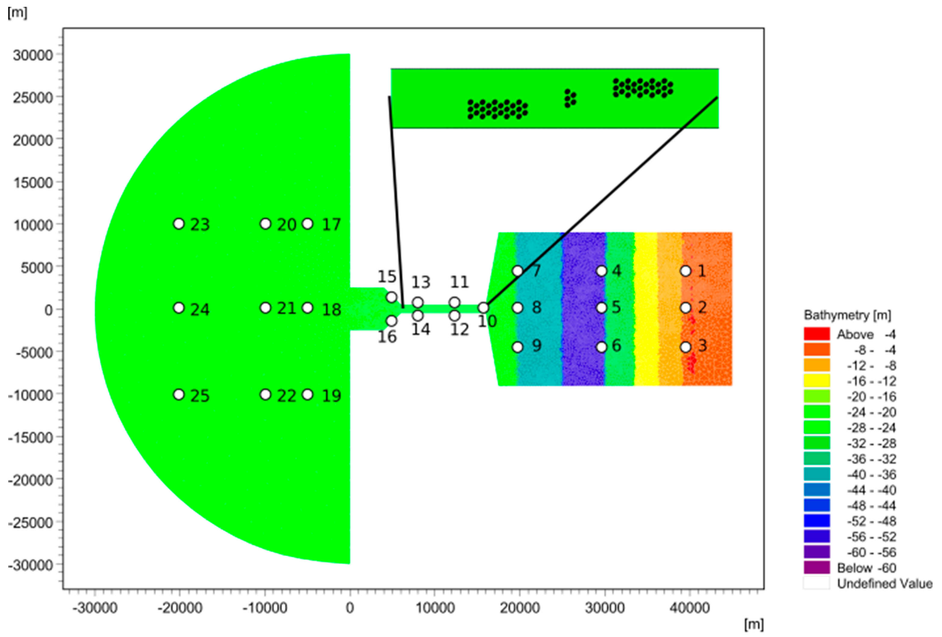
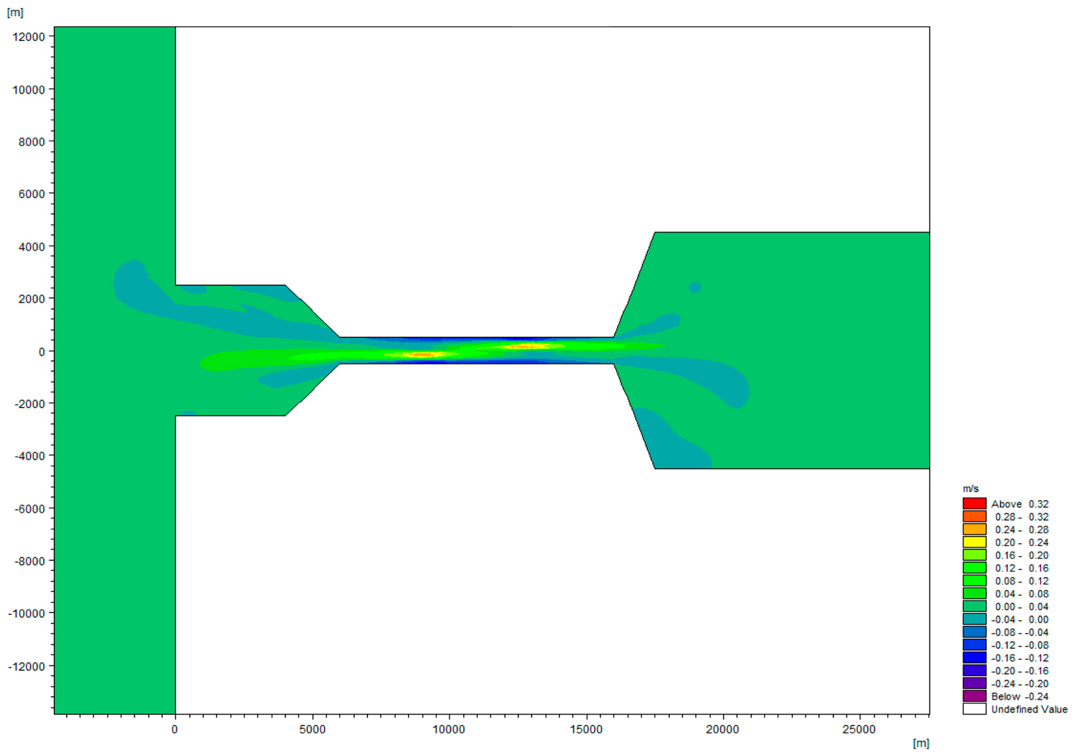
2.1. Hydrodynamic Model
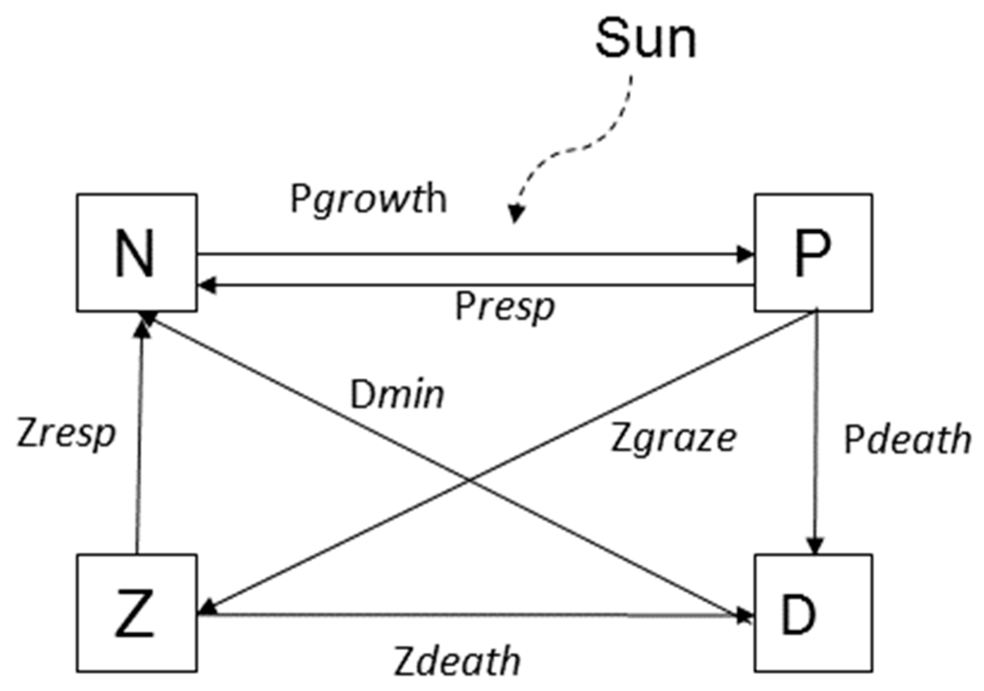
2.2. NPZD Model
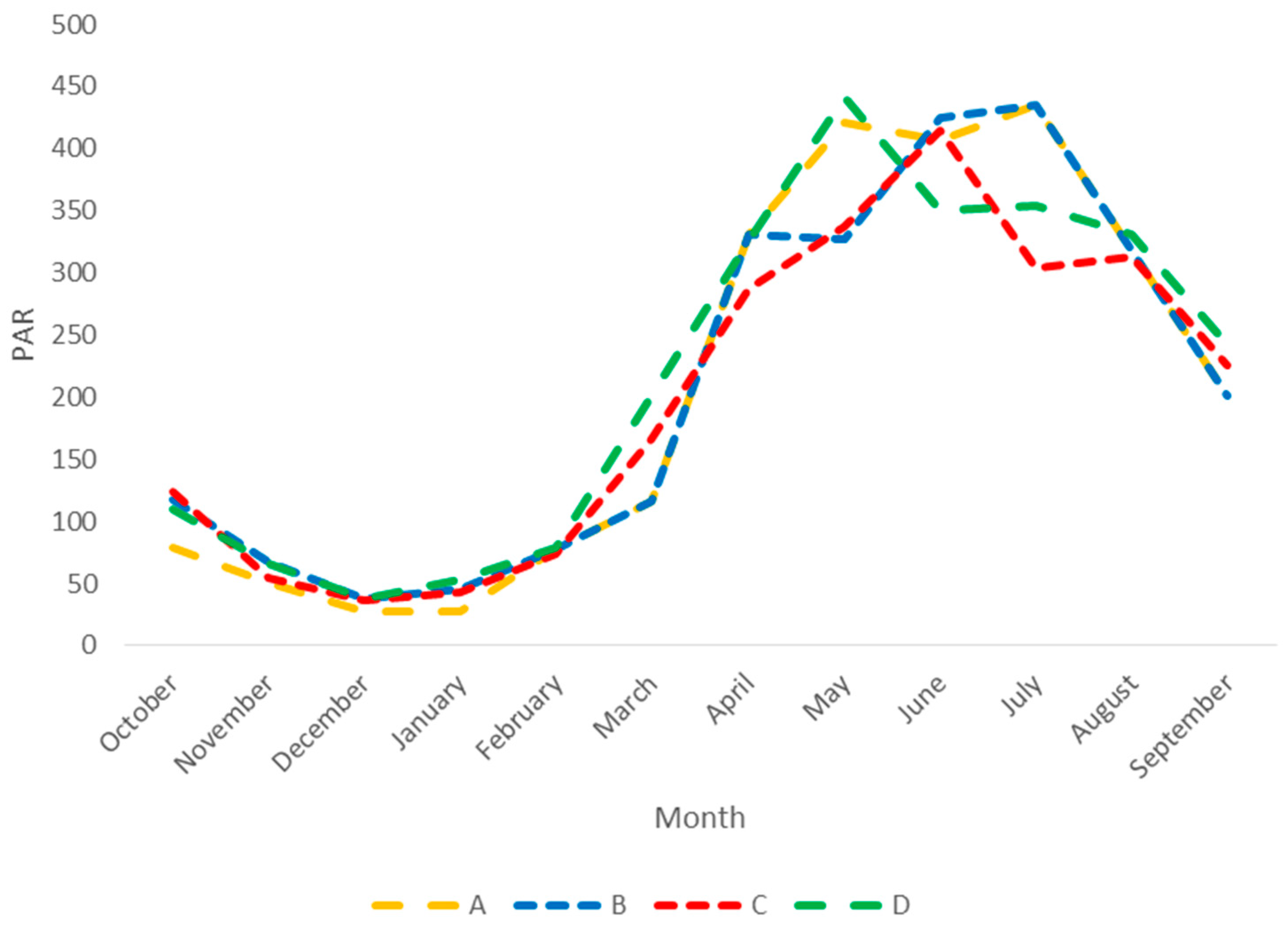
2.3. Data and Simulation
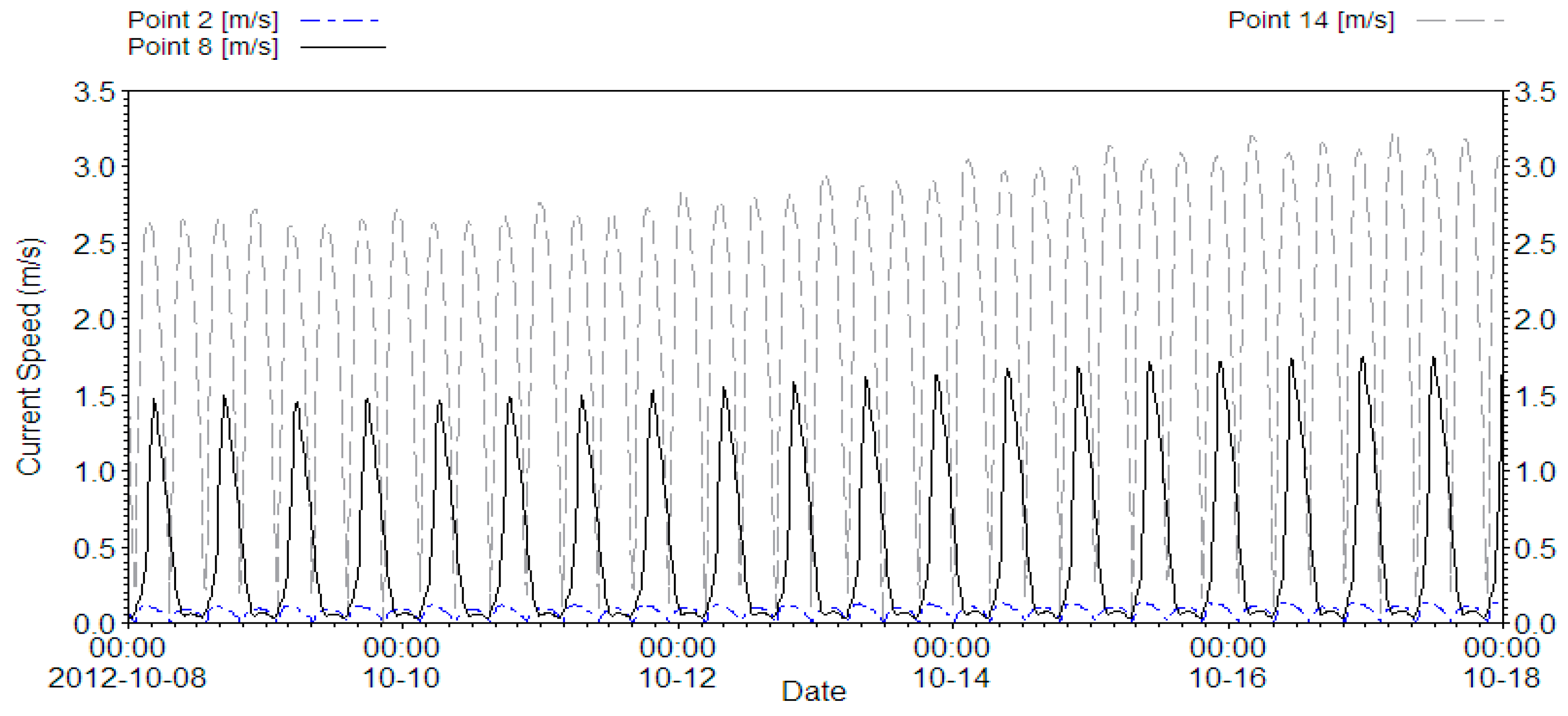
2.4. Analysis
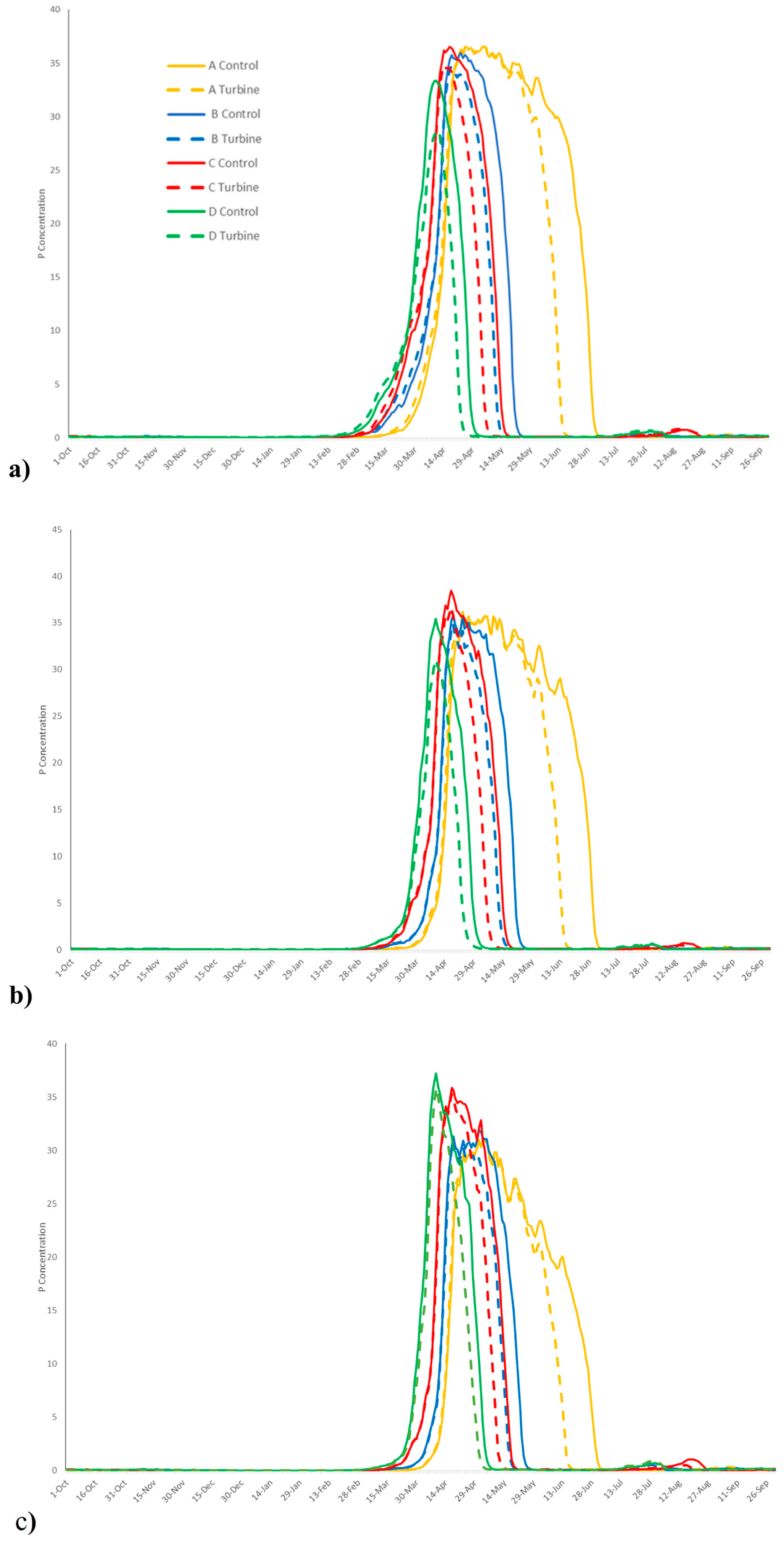
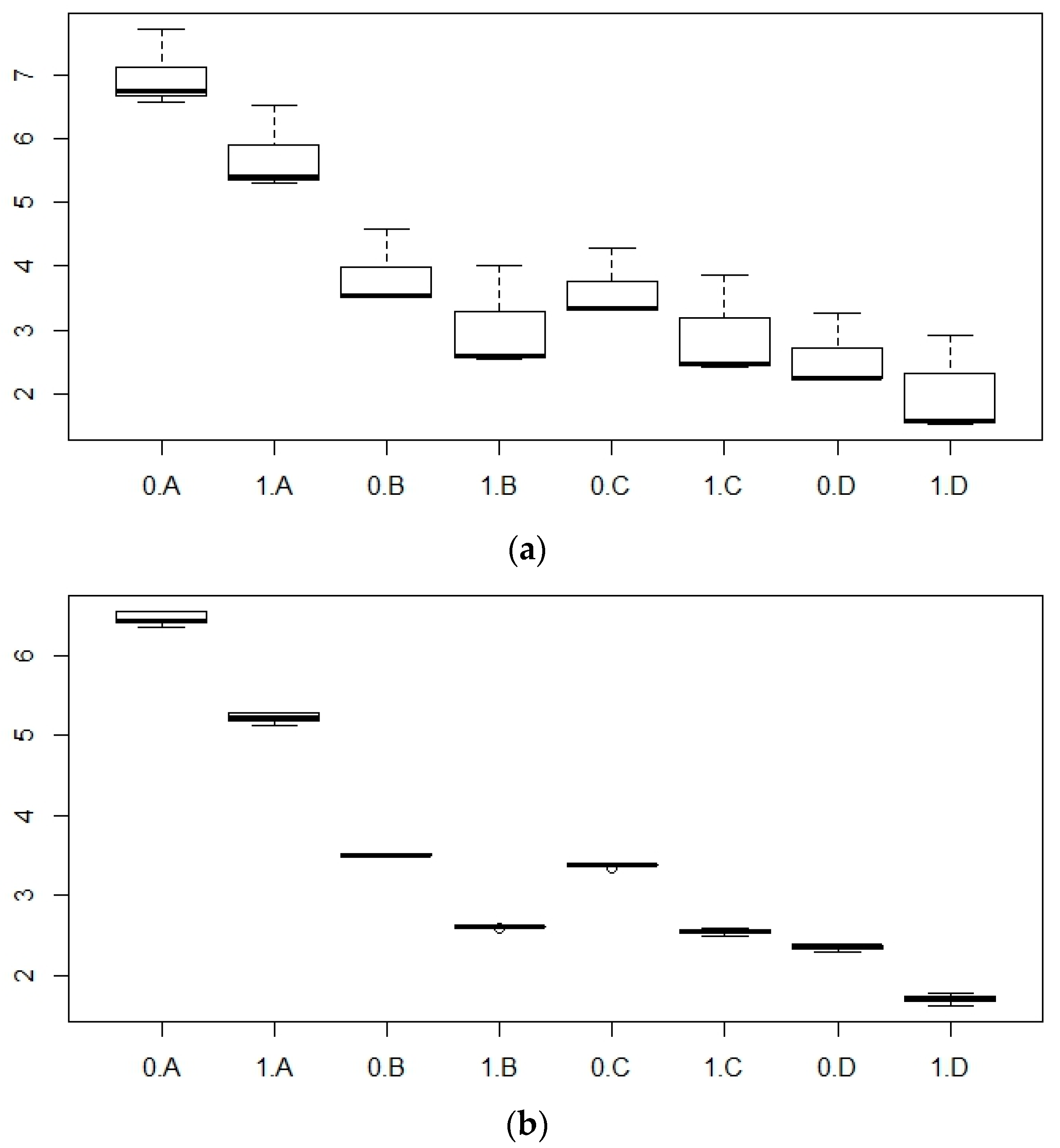
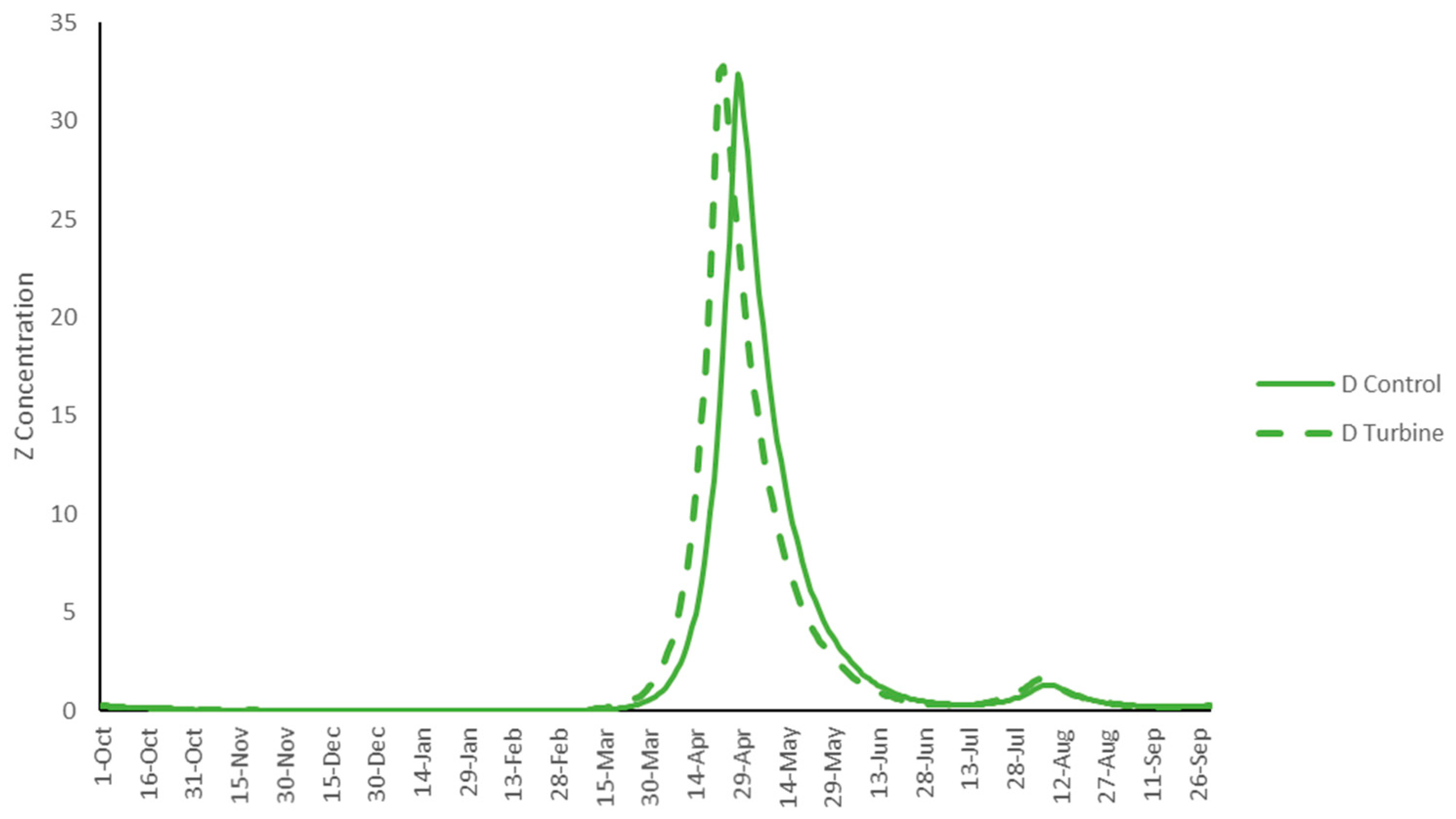
3. Results
4. Discussion
Author Contributions
Funding
Conflicts of Interest
References
- The Crown Estate. UK Wave and Tidal Key Resource Areas Project; The Crown Estate: London, UK, 2012. [Google Scholar]
- Cameron, B.; Farwell, S.; Oldreive, M. Establishing marine renewable energy legislation in Nova Scotia, Canada. In Proceedings of the 11th European Wave & Tidal Energy Conference, Nantes, France, 6–11 September 2015. [Google Scholar]
- Magagna, D.; Uihlein, A.; Silva, M.; Raventos, A. Wave and tidal energy in Europe: Assessing present technologies. In Proceedings of the 11th European Wave & Tidal Energy Conference, Nantes, France, 6–11 September 2015. [Google Scholar]
- Magagna, D.; Monfardini, R.; Uihlein, A. JRC Ocean Energy Status Report: 2016 Edition; EUR 28407 EN; Publications Office of the European Union: Luxembourg City, Luxembourg, 2016. [Google Scholar]
- Boehlert, G.W.; Gill, A.B. Environmental and ecological effects of ocean renewable energy development. A current synthesis. Oceanography 2010, 23, 68–81. [Google Scholar] [CrossRef] [Green Version]
- Kadiri, M.; Ahmadian, R.; Bockelmann-Evans, B.; Rauen, W.; Falconer, R. A review of the potential water quality impacts of tidal renewable energy systems. Renew. Sustain. Energy Rev. 2012, 16, 329–341. [Google Scholar] [CrossRef]
- Maclean, I.M.D.; Inger, R.; Benson, D.; Booth, C.G.; Embling, C.B.; Grecian, W.J.; Heymans, J.J.; Plummer, K.E.; Shackshaft, M.; Sparling, C.E.; et al. Resolving issues with environmental impact assessment of marine renewable energy installations. Front. Mar. Sci. 2014, 1, 75. [Google Scholar] [CrossRef] [Green Version]
- Shields, M.A.; Woolf, D.K.; Grist, E.P.M.; Kerr, S.A.; Jackson, A.C.; Harris, R.E.; Bell, M.C.; Beharie, R.; Want, A.; Osalusi, E.; et al. Marine renewable energy: The ecological implications of altering the hydrodynamics of the marine environment. Ocean Coast. Manag. 2011, 54, 2–9. [Google Scholar] [CrossRef]
- Shields, M.A.; Payne, A.I.L. Marine Renewable Energy Technology and Environmental Interactions; Springer Science and Business Media: Dordrecht, The Netherlands, 2014. [Google Scholar]
- Martin-Short, R.; Hill, J.; Kramer, S.C.; Avdis, A.; Allison, P.A.; Piggott, M.D. Tidal resource extraction in the Pentland Firth, UK: Potential impacts on flow regime and sediment transport in the Inner Sound of Stroma. Renew. Energy 2015, 76, 596–607. [Google Scholar] [CrossRef]
- Neill, S.P.; Litt, E.J.; Couch, S.J.; Davies, A.G. The impact of tidal stream turbines on large-scale sediment dynamics. Renew. Energy 2009, 34, 2803–2812. [Google Scholar] [CrossRef]
- Thompson, D.; Hall, A.J.; Lonergan, M.; McConnell, B.; Northridge, S. Current status of knowledge of effects of offshore renewable energy generation devices on marine mammals and research requirements. In Report to Scottish Government; Scottish Government: Edinburgh, UK, 2013. [Google Scholar]
- Hastie, G.D.; Russell, D.J.F.; Lepper, P.; Elliott, J.; Wilson, B.; Benjamins, S.; Thompson, D. Harbour seals avoid tidal turbine noise: Implications for collision risk. J. Appl. Ecol. 2017, 1–10. [Google Scholar] [CrossRef]
- Hammar, L.; Ehnberg, J. Who should be afraid of a tidal turbine—The good, the bad or the ugly? In Proceedings of the 10th European Wave and Tidal Energy Conference Proceedings, Aalborg, Denmark, 2–5 September 2013. [Google Scholar]
- Hammar, L.; Eggertsen, L.; Andersson, S.; Ehnberg, J.; Arvidsson, R.; Gullstroem, M.; Molander, S. A Probabilistic model for hydrokinetic turbine collision risks: Exploring Impacts on Fish. PLoS ONE 2015, 10, e0117756. [Google Scholar] [CrossRef] [PubMed]
- Williamson, B.; Fraser, S.; Blondel, P.; Bell, P.; Waggitt, J.; Scott, B. Multisensor Acoustic Tracking of Fish and Seabird Behavior Around Tidal Turbine Structures in Scotland. IEEE J. Ocean. Eng. 2017, 42, 948–965. [Google Scholar] [CrossRef]
- Adams, T.P.; Miller, R.G.; Aleynik, D.; Burrows, M.T. Offshore marine renewable energy devices as stepping stones across biogeographical boundaries. J. Appl. Ecol. 2014, 51, 330–338. [Google Scholar] [CrossRef]
- Kregting, L.; Elsäßer, B.; Kennedy, R.; Smyth, D.; O’Carroll, J.; Savidge, G. Do changes in current flow as a result of arrays of tidal turbines have an effect on benthic communities? PLoS ONE 2016, 11, e0161279. [Google Scholar] [CrossRef] [PubMed]
- Couch, S.J.; Bryden, I.G. Large-scale physical response of the tidal system to energy extraction and its significance for informing environmental and ecological impact assessment. In Proceedings of the Oceans 2007-Europe International Conference, Aberdeen, UK, 18–21 June 2007. [Google Scholar]
- Yang, Z.; Wang, T. Assessment of Energy Removal Impacts on Physical Systems: Development of MHK Module and Analysis of Effects on Hydrodynamics. Pacific Northwest National Laboratory. Available online: https://tethys.pnnl.gov/sites/default/files/publications/Development_of_MHK_Module_and_Analysis.pdf (accessed on 22 May 2018).
- Falkowski, P.G.; Raven, J.A. Aquatic Photosynthesis; Princeton University Press: Princeton, NJ, USA, 2007. [Google Scholar]
- Franks, P. NPZ models of plankton dynamics: Their construction, coupling to physics, and application. J. Oceanogr. 2002, 58, 379–387. [Google Scholar] [CrossRef]
- Ji, R.; Davis, C.; Chen, C.; Beardsley, R. Influence of local and external processes on the annual nitrogen cycle and primary productivity on Georges Bank: A 3-D biological-physical modeling study. J. Mar. Syst. 2008, 73, 31–47. [Google Scholar] [CrossRef]
- Hannah, C.; Vezina, A.; John, M.S. The case for marine ecosystem models of intermediate complexity. Prog. Oceanogr. 2010, 84, 121–128. [Google Scholar] [CrossRef] [Green Version]
- Longdill, P. Environmentally Sustainable Aquaculture: An eco-Physical Perspective. Ph.D. Thesis, The University of Waikato, Hamilton, New Zealand, 2007. [Google Scholar]
- Wild-Allen, K.; Herzfeld, M.; Thompson, P.A.; Rosebrock, U.; Parslow, J.; Volkman, J.K. Applied coastal biogeochemical modelling to quantify the environmental impact of fish farm nutrients and inform managers. J. Mar. Syst. 2010, 81, 134–147. [Google Scholar] [CrossRef]
- Wild-Allen, K.; Thompson, P.A.; Volkman, J.K.; Parslow, J. Use of a coastal biogeochemical model to select environmental monitoring sites. J. Mar. Syst. 2011, 88, 120–127. [Google Scholar] [CrossRef]
- Van der Molen, J.; Smith, H.C.M.; Lepper, P.; Limpenny, S.; Rees, J. Predicting the large-scale consequences of offshore wind turbine array development on a North Sea ecosystem. Cont. Shelf Res. 2014, 85, 60–72. [Google Scholar] [CrossRef] [Green Version]
- Van der Molen, J.; Ruardij, P.; Greenwood, N. Potential environmental impact of tidal energy extraction in the Pentland Firth at large spatial scales: Results of a biogeochemical model. Biogeosciences 2016, 13, 2593–2609. [Google Scholar] [CrossRef] [Green Version]
- Wang, T.; Yang, Z.; Copping, A. A modelling study of the potential water quality impacts from in-stream tidal energy extraction. Estuaries Coasts 2015, 38 (Suppl. 1), S173–S186. [Google Scholar] [CrossRef]
- Walkington, I.; Burrows, R. Modelling tidal stream power potential. Appl. Ocean Res. 2009, 31, 239–245. [Google Scholar] [CrossRef]
- Kramer, S.C.; Piggott, M.D.; Hill, J.; Kregting, L.; Pritchard, D.; Elsäßer, B. The modelling of tidal turbine farms using multi-scale, unstructured mesh models. In Proceedings of the 2nd International Conference on Environmental Interactions of Marine Renewable Energy Technologies (EIMR2014), Kirkwall, Orkney, 28 April–02 May 2014. [Google Scholar]
- Kregting, L.; Elsäßer, B. A hydrodynamic framework for Strangford Lough Part 1: Tidal Model. J. Mar. Sci. Eng. 2014, 2, 46–65. [Google Scholar] [CrossRef]
- Simpson, J.S.; Hunter, J.R. Fronts in the Irish Sea. Nature 1974, 250, 404–406. [Google Scholar] [CrossRef]
- Thorpe, S.A. An Introduction to Ocean Turbulence; Cambridge University Press: New York, NY, USA, 2007. [Google Scholar]
- Fennel, W.; Neumann, T. Introduction to the Modelling of Marine Ecosystems; Elsevier: New York, NY, USA, 2015. [Google Scholar]
- Herman, J.; Shen, J.; Huang, J. Tidal Flushing Characteristics in Virginia’s Tidal Embayments. In Virginia Coastal Zone Management Program; Virginia Department of Environmental Quality: Richmond, VA, USA, 2007. [Google Scholar]
- Groemping, U. Relative Importance for Linear Regression in R: The package realimpo. J. Stat. Softw. 2006, 17, 1–27. [Google Scholar]
- White, J.W.; Rassweiler, A.; Samhouri, J.F.; Stier, A.C.; White, C. Ecologists should not use statistical significance tests to interpret simulation model results. Oikos 2014, 123, 385–388. [Google Scholar] [CrossRef]
- Lindeman, R.H.; Merenda, P.F.; Gold, R.Z. Introduction to Bivariate and Multivariate Analysis; Scott Foresman: Glenview, IL, USA, 1980. [Google Scholar]
- Cloern, J.E.; Schraga, T.S.; Lopez, C.B.; Knowles, N.; Labiosa, R.G.; Dugdale, R. Climate anomalies generate an exceptional dinoflagellate bloom in San Francisco Bay. Geophys. Res. Lett. 2005, 32, 172–180. [Google Scholar] [CrossRef]
- Philippart, C.J.M.; van Iperen, J.M.; Cadée, G.C.; Zuur, A.F. Long-term field observations on seasonality in chlorophyll-a concentrations in a shallow coastal marine ecosystem, the Wadden Sea. Estuar. Coasts 2010, 33, 286–294. [Google Scholar] [CrossRef]
- Culley, D.M.; Funke, S.W.; Kramer, S.C.; Piggott, M.D. Integration of cost modelling within the micro-siting design optimisation of tidal turbine arrays. Renew. Energy 2016, 85, 215–227. [Google Scholar] [CrossRef]
- Stansby, P.; Stallard, T. Fast optimisation of tidal stream turbine positions for power generation in small arrays with low blockage based on superposition of self-similar far-wake velocity deficit profiles. Renew. Energy 2016, 92, 366–375. [Google Scholar] [CrossRef]
- Vanhellemont, Q.; Ruddick, K. Turbid wakes associated with offshore wind turbines observed with Landsat 8. Remote Sens. Environ. 2014, 145, 105–115. [Google Scholar] [CrossRef]
- Savidge, G.; Ainsworth, D.; Bearhop, S.; Christen, N.; Elsäßer, B.; Fortune, F.; Inger, R.; Kennedy, R.; McRobert, A.; Plummer, K.E.; et al. Strangford Lough and the SeaGen tidal turbine. In Marine Renewable Energy Technology and Environmental Interactions; Shields, M.A., Payne, A.I.L., Eds.; Humanity and the Sea: Dordrecht, The Netherland, 2014; pp. 153–172. [Google Scholar]


| Domain | Length (m) | Width (m) | Depth (m) |
|---|---|---|---|
| Coastal ocean | 30,000 | 60,000 | 20 |
| Channel | 10,000 | 1000 | 20 |
| Basin | 30,000 | 17,000 | 60 |
| Name | Type | Process | Description |
|---|---|---|---|
| N | State | Pgrowth + Prespiration + Dmineralization + Zexcretion | Nutrient concentration |
| P | State | Pgrowth − Prespiration − Pdeath − Pgraze | Phytoplankton concentration |
| Z | State | Pgraze − Zdeath − Zexcretion | Zooplankton concentration |
| D | State | Pdeath − Dmineralization + Zdeath | Detritus concentration |
| Prespiration | aux | lpn*P | Phytoplankton respiration |
| Pdeath | aux | lpd*P | Phytoplankton mortality |
| Pgraze | aux | gP*Z*Epz | Grazing of zooplankton on phytoplankton |
| Pgrowth | aux | Rmaxa*fN*P | Growth of phytoplankton |
| Zdeath | aux | lzd*Z | Zooplankton mortality |
| Zexcretion | aux | lzn*Z | Zooplankton excretion |
| Dmineralization | aux | ldn*D | Detritus mineralization |
| fI | aux | Light limiting function for phytoplankton growth | |
| I | aux | Max(0.00001, ) | Average light intensity I from the surface to the depth dz. Lambert–Beer expression is integrated over depth. |
| gP | aux | Gmax*fP | Zooplankton grazing rate |
| fP | aux | IF(P > Pt), THEN, ELSE 0 | Phytoplankton limitation function |
| Rmaxa | aux | Rmax*fI | Maximum growth rate of phytoplankton light dependent |
| fN | aux | Nutrient limitation function | |
| Kn | const | 0.025 | Half saturation constant |
| lpn | const | 0.1 | Phytoplankton respiration |
| lpd | const | 0.001 | Phytoplankton mortality rate |
| ldn | const | 0.005 | Detritus mineralization rate |
| gmax | const | 0.4 | Maximum grazing rate of zooplankton |
| lzd | const | 0.05 | Zooplankton mortality rate |
| lzn | const | 0.035 | Zooplankton excretion rate |
| rmax | const | 1 | Phytoplankton maximal growth rate |
| eta | const | 0.34 | Light attenuation factor in water column |
| Epz | const | 0.6 | Feeding efficiency of zooplankton |
| Pt | const | 0.04 | Phytoplankton Threshold for zooplankton feeding |
| Kp | const | 0.2 | Half Saturation constant for Phytoplankton |
| dz | forcing | Depth | |
| ios | forcing | PAR |
| Solar Radiation | Basin (g/m3) | Channel (g/m3) | Open Ocean (g/m3) | ||
|---|---|---|---|---|---|
| Without TED | A | Average concentration | 6.94 | 6.46 | 4.87 |
| Peak concentration | 37.32 | 36.19 | 31.13 | ||
| B | Average concentration | 3.81 | 3.51 | 3.11 | |
| Peak concentration | 36.81 | 35.92 | 32.62 | ||
| C | Average concentration | 3.59 | 3.38 | 3.25 | |
| Peak concentration | 37.15 | 38.48 | 36.07 | ||
| D | Average concentration | 2.52 | 2.35 | 2.60 | |
| Peak concentration | 33.60 | 35.43 | 37.23 | ||
| Largest difference between scenarios A–D | Average concentration | 4.42 | 4.11 | 2.27 | |
| Peak concentration | 3.72 | 3.05 | 5.92 | ||
| With TED | A | Average concentration | 5.65 | 5.23 | 4.08 |
| Peak concentration | 37.13 | 36.07 | 31.28 | ||
| B | Average concentration | 2.95 | 2.61 | 2.47 | |
| Peak concentration | 35.42 | 34.98 | 31.96 | ||
| C | Average concentration | 3.73 | 2.55 | 2.62 | |
| Peak concentration | 33.02 | 36.71 | 35.31 | ||
| D | Average annual concentration | 1.94 | 1.70 | 2.09 | |
| Peak concentration | 29.27 | 31.03 | 35.85 | ||
| Largest difference between scenarios A–D | Average concentration | 3.72 | 3.52 | 1.99 | |
| Peak concentration | 7.85 | 5.67 | 4.57 | ||
| Difference in raw value and percentage between scenarios No TEDs and TEDs; (TED—No TED)/ No TED | A | Average concentration | −1.28 (−18.6%) | −1.23 (−19%) | −0.79 (−16.2%) |
| Peak concentration | −0.19 (−0.5%) | −0.12 (−0.3%) | −0.04 (−0.5%) | ||
| B | Average concentration | −0.85 (−22.6%) | −0.89 (−25.6%) | −0.63 (−20.6%) | |
| Peak concentration | −1.39 (−3.8%) | −0.93 (−2.6%) | −0.66 (−2.0%) | ||
| C | Average concentration | 0.14 (3.9%) | −0.83 (−24.6%) | −0.63 (−19.4%) | |
| Peak concentration | −4.13 (−11.1%) | −1.77 (−4.6%) | −0.76 (−2.1%) | ||
| D | Average concentration | −0.58 (−23.0%) | −0.65 (−27.7%) | −0.51 (−19.6%) | |
| Peak concentration | −4.32 (−12.9%) | −4.39 (−12.4%) | −1.38 (−3.7%) |
| Variable | Estimate | Std. Error | Variation Explained (%) | ||
|---|---|---|---|---|---|
| P mean Total variation explained: 87.14% | Intercept | 6.23 | 0.09 | ||
| TED | Turbine | −0.79 | 0.07 | 7.8 | |
| Area | Channel | −0.31 | 0.09 | 3.6 | |
| Open Ocean | −0.64 | 0.08 | |||
| PAR | B | −2.44 | 0.10 | 75.6 | |
| C | −2.47 | 0.10 | |||
| D | −3.30 | 0.10 | |||
| P max Total variation explained: 27.24% | Intercept | 35.88 | 0.43 | ||
| TED | Turbine | −1.46 | 0.33 | 7.4 | |
| Area | Channel | 0.36 | 0.41 | 7.0 | |
| Open Ocean | −1.29 | 0.39 | |||
| PAR | B | −0.23 | 0.46 | 12.8 | |
| C | 1.63 | 0.46 | |||
| D | −1.01 | 0.46 |
© 2018 by the authors. Licensee MDPI, Basel, Switzerland. This article is an open access article distributed under the terms and conditions of the Creative Commons Attribution (CC BY) license (http://creativecommons.org/licenses/by/4.0/).
Share and Cite
Schuchert, P.; Kregting, L.; Pritchard, D.; Savidge, G.; Elsäßer, B. Using Coupled Hydrodynamic Biogeochemical Models to Predict the Effects of Tidal Turbine Arrays on Phytoplankton Dynamics. J. Mar. Sci. Eng. 2018, 6, 58. https://doi.org/10.3390/jmse6020058
Schuchert P, Kregting L, Pritchard D, Savidge G, Elsäßer B. Using Coupled Hydrodynamic Biogeochemical Models to Predict the Effects of Tidal Turbine Arrays on Phytoplankton Dynamics. Journal of Marine Science and Engineering. 2018; 6(2):58. https://doi.org/10.3390/jmse6020058
Chicago/Turabian StyleSchuchert, Pia, Louise Kregting, Daniel Pritchard, Graham Savidge, and Björn Elsäßer. 2018. "Using Coupled Hydrodynamic Biogeochemical Models to Predict the Effects of Tidal Turbine Arrays on Phytoplankton Dynamics" Journal of Marine Science and Engineering 6, no. 2: 58. https://doi.org/10.3390/jmse6020058