Storm Surge and Wave Impact of Low-Probability Hurricanes on the Lower Delaware Bay—Calibration and Application


Abstract
:1. Introduction
Deterministic vs. Probabilistic
2. Methodology
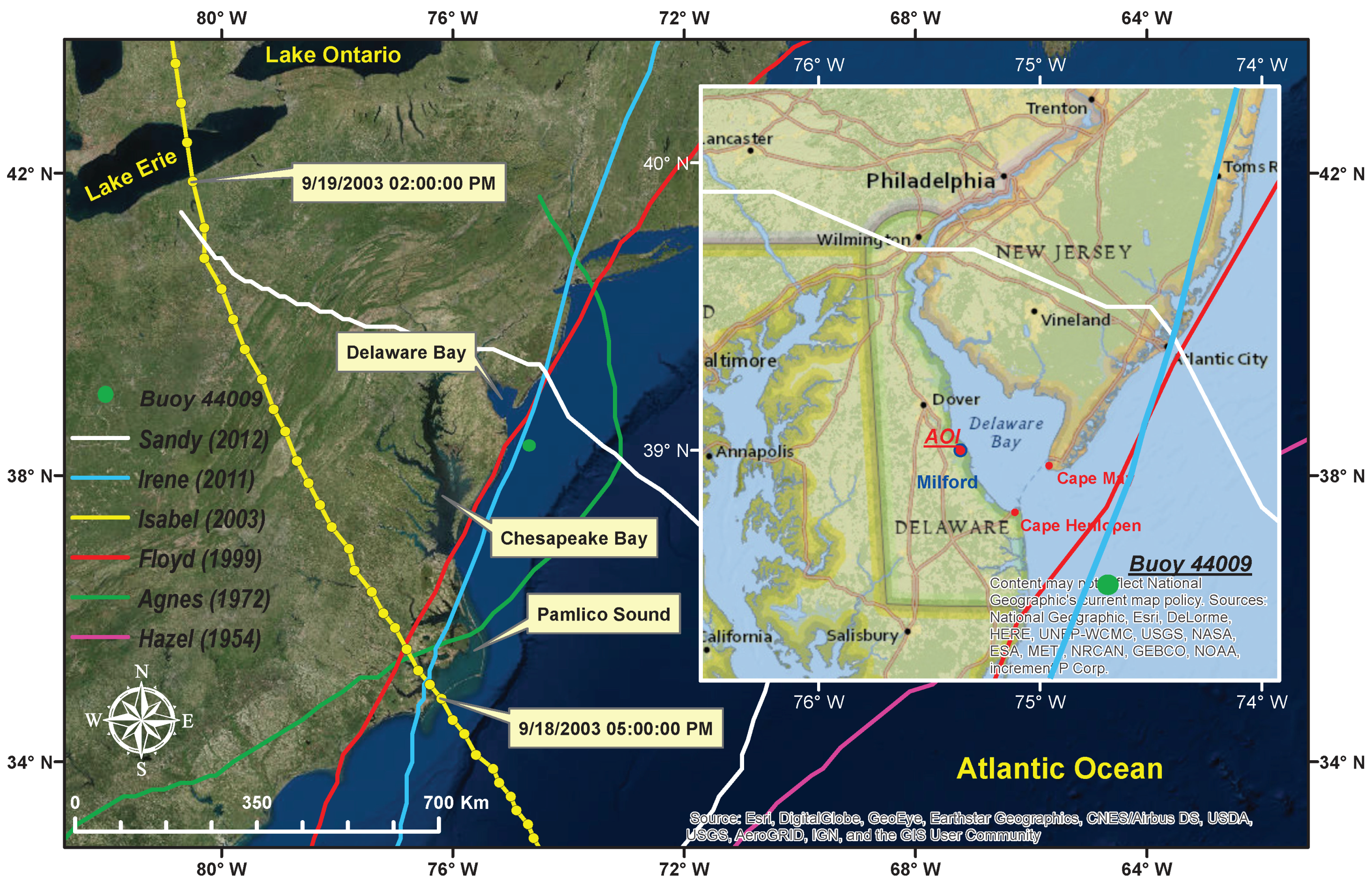
2.1. Study Area
2.2. Computational Models
2.2.1. Delft3D-FLOW Module
2.2.2. Delft3D-WAVE Module
2.2.3. Delft3D-WES Module
2.3. Model Configurations
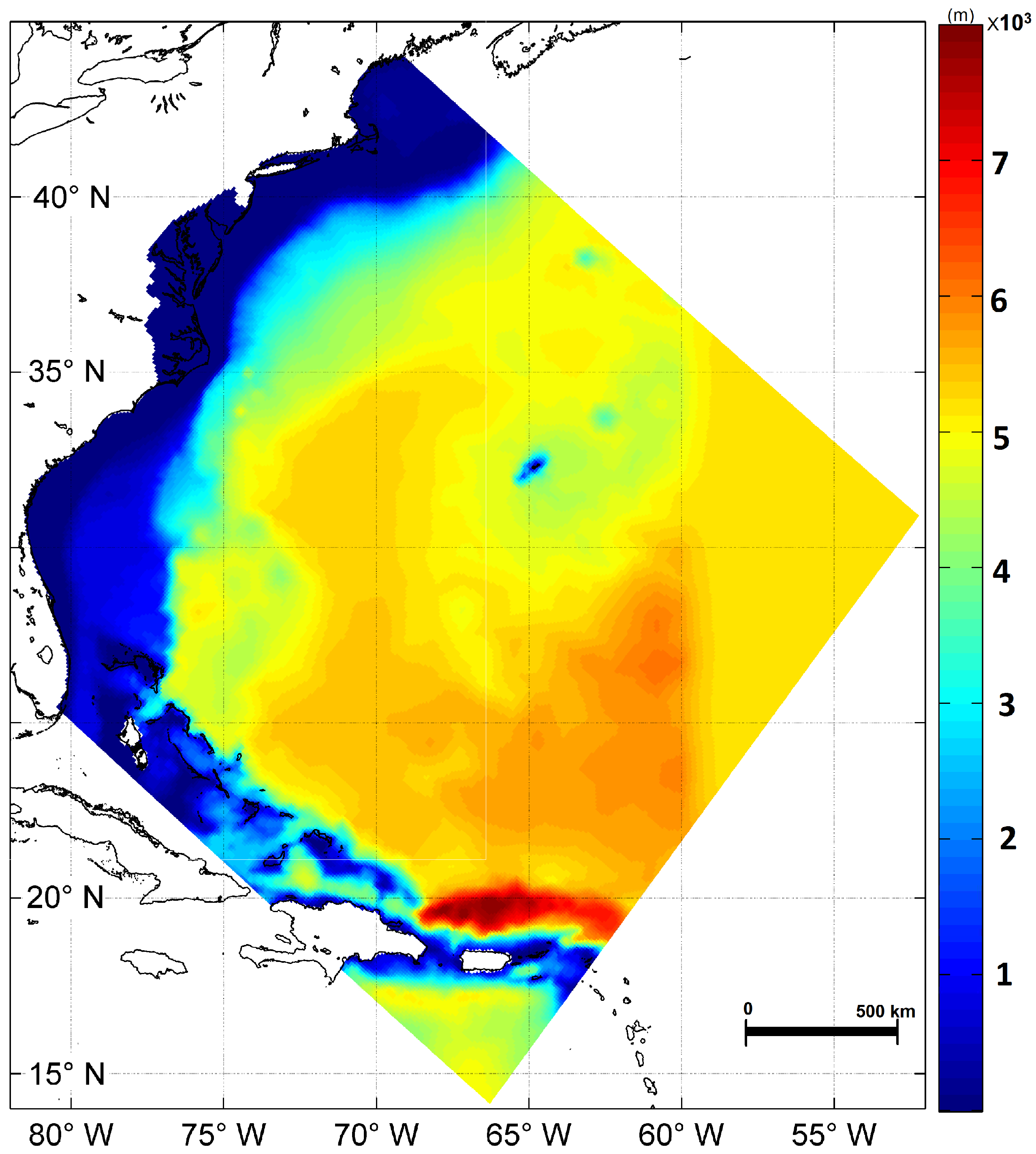
2.3.1. Model Domain
2.3.2. Overall Domain
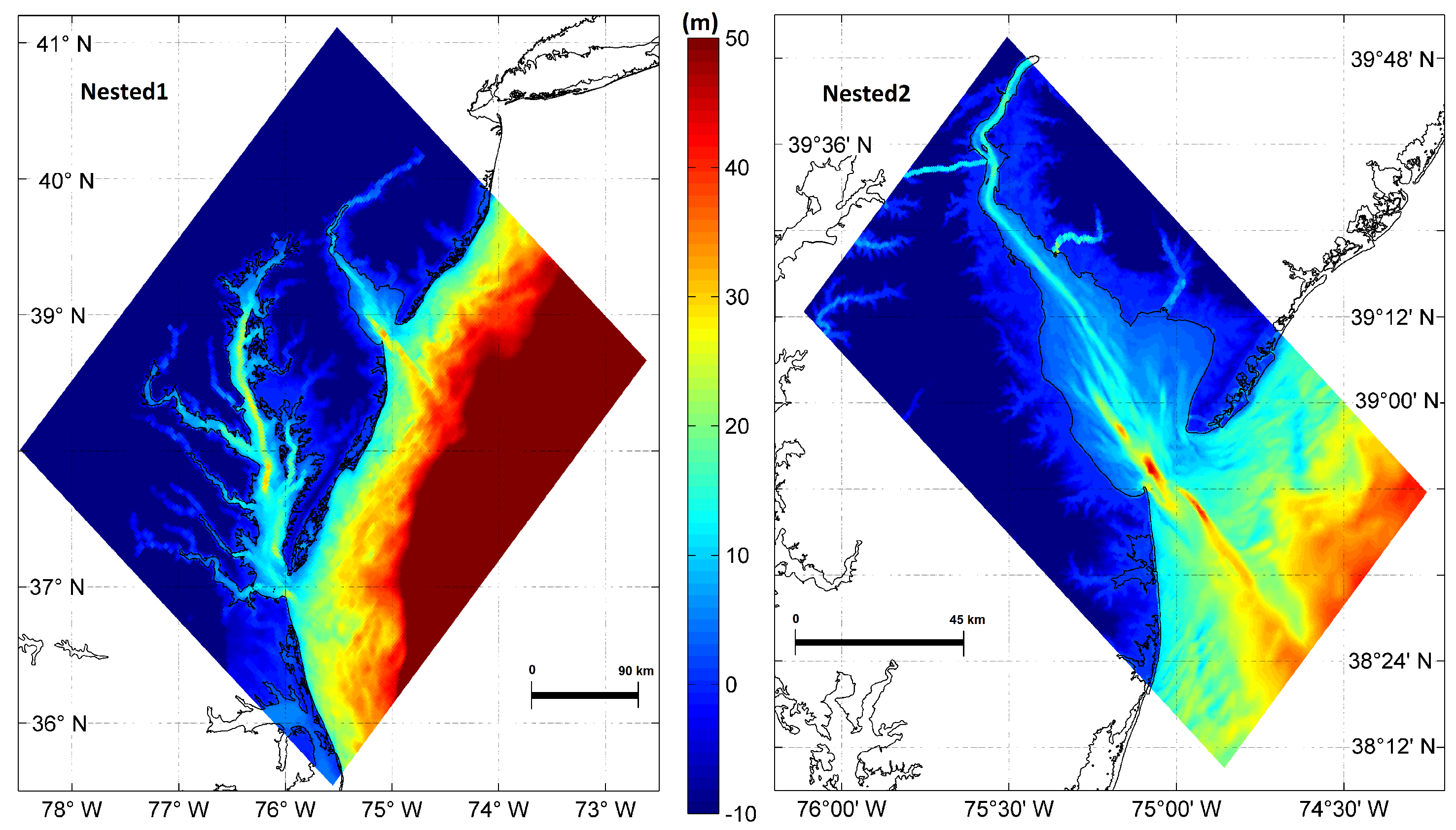
2.3.3. Nested Domains
2.3.4. Standard Setting
2.4. Model Forcing
2.4.1. River Discharges
2.4.2. Tides
2.4.3. Meteorological Forcing—Wind Field
2.4.4. Delft3D-WES Setting
2.4.5. Historical Storm
2.4.6. Synthetic Storms
2.5. Model Calibration and Sensitivity
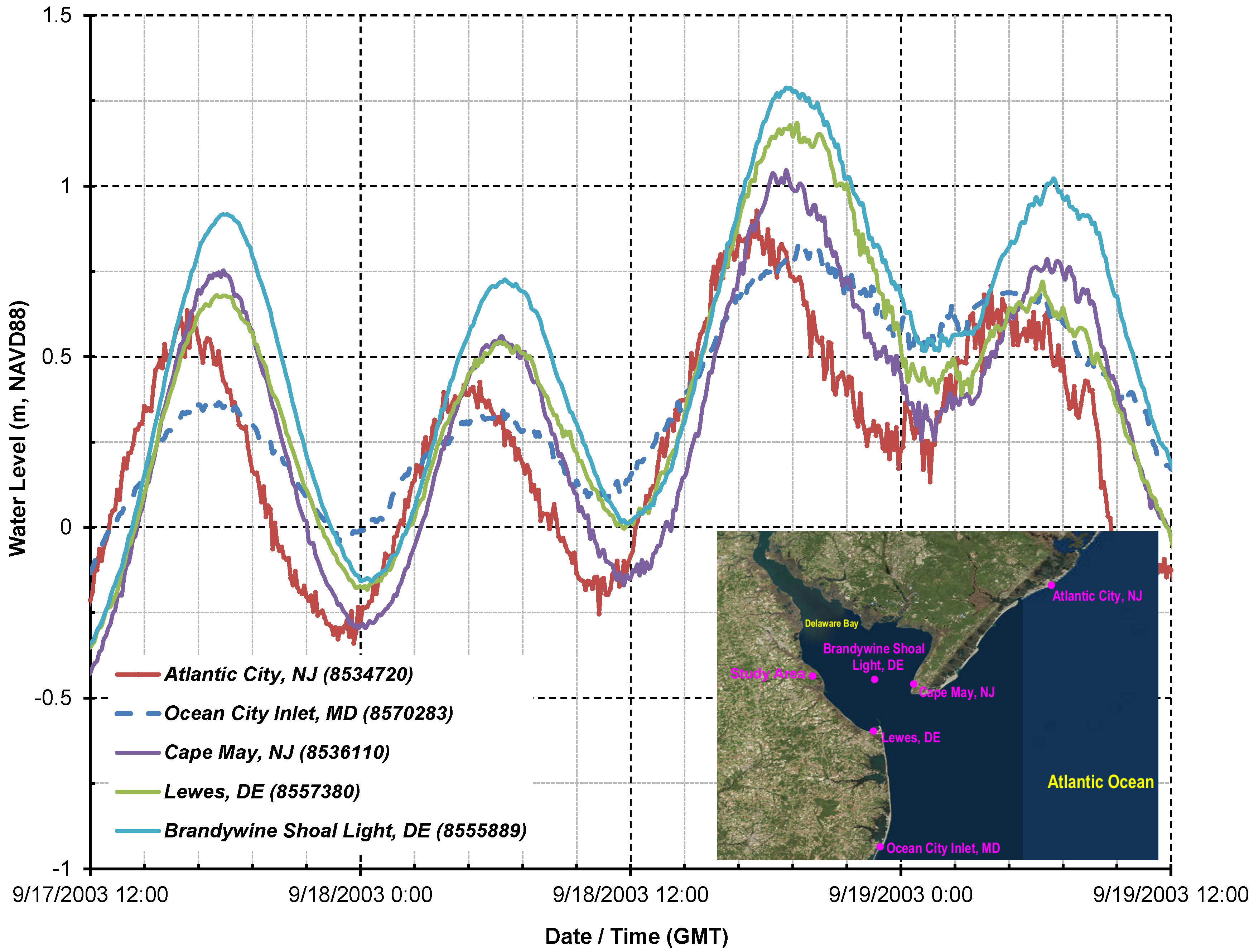
2.5.1. Observations
2.5.2. Calibration Model Comparison
3. Results and Discussion
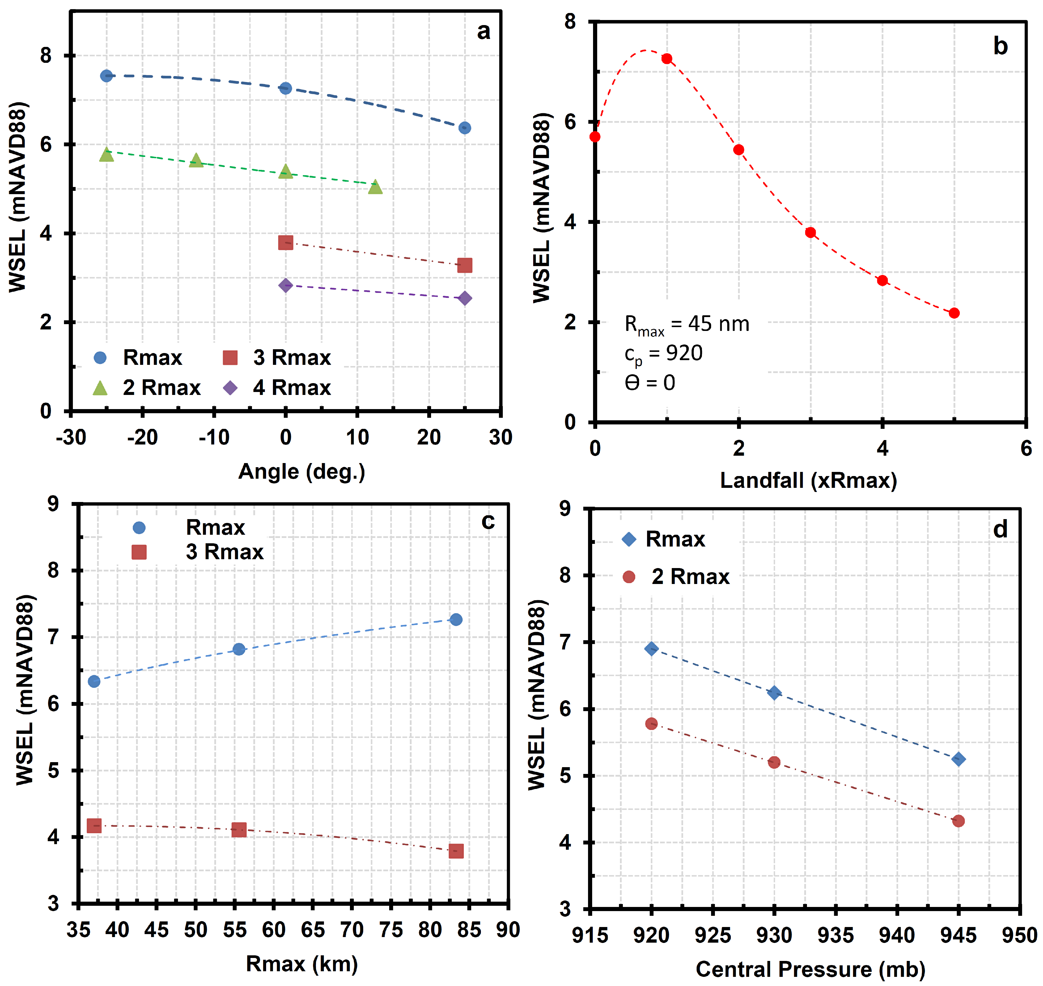
- Of the tracks with the same landfall location, central pressure (), radius of maximum winds (), and maximum wind speed () those that rotated counterclockwise from the axis of the Delaware Bay resulted in the highest WSEL (see Figure 12a). Tracks passing from the axis of the Delaware Bay (i.e., landfall equal to zero) were the only exceptions. Such orientation pushes the water in a more straightforward path toward the site.
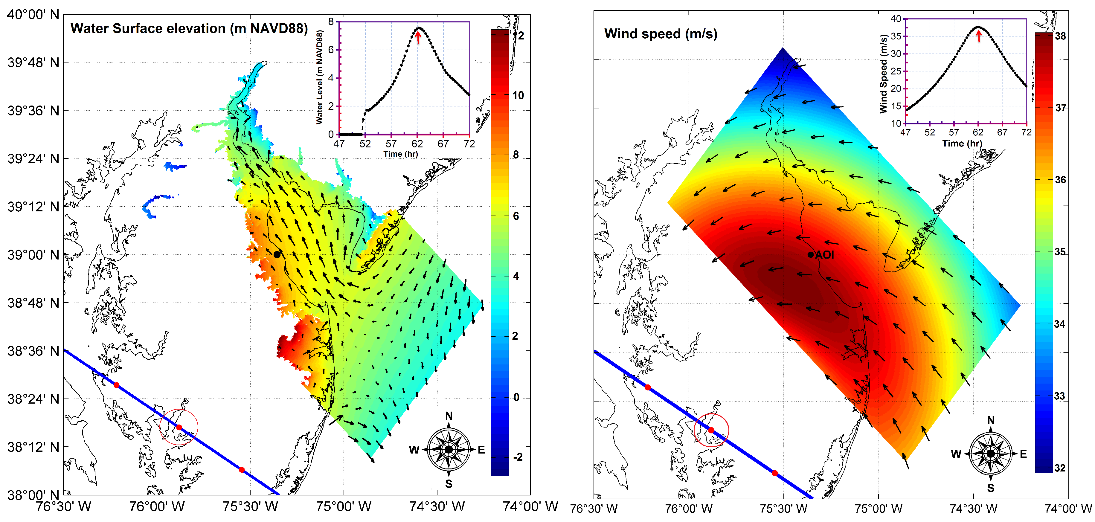
- For tracks with the same angle or orientation, , , and ; those with a landfall location spaced 1 west of the study area resulted in highest WSEL (see Figure 12b). Increasing the distance beyond that reduces the water levels. This could be attributed to locating the maximum winds closest to the AOI and is similar to findings from others, such as Irish et al. [58].
- Keeping all the parameters constant except , if the hurricane makes landfall on the west side of the site at a distance 1 away, the WSEL increases with increasing the (see Figure 12c). However, this would not be the case for tracks located farther from the AOI. The same explanation as given in the above article again applies.
- Results show a linear relation between the central pressure and storm surge (see Figure 12d). Decreasing the central pressure increases the pressure drop, which eventually enhances maximum wind speeds and results in higher impacts during its passage. Each 1 millibar drop in the central pressure results in approximately 0.6 m increase in storm surge.
4. Conclusions
Acknowledgments
Conflicts of Interest
References
- Emanuel, K. Climate and Tropical Cyclone Activity: A New Model Downscaling Approach. J. Clim. 2006, 19, 4797–4802. [Google Scholar] [CrossRef]
- Lin, N.; Smith, J.A.; Villarini, G.; Marchok, T.P.; Baeck, M.L. Modeling Extreme Rainfall, Winds, and Surge from Hurricane Isabel (2003). Weather Forecast. 2010, 25, 1342–1361. [Google Scholar] [CrossRef]
- Garzon, J.L.; Ferreira, C.M. Storm Surge Modeling in Large Estuaries: Sensitivity Analyses to Parameters and Physical Processes in the Chesapeake Bay. J. Mar. Sci. Eng. 2016, 4, 45. [Google Scholar] [CrossRef]
- Emanuel, K.; Sobel, A. Response of Tropical Sea Surface Temperature, Precipitation, and Tropical Cyclone—Related Variables to Changes in Global and Local Forcing. J. Adv. Model. Earth Syst. 2013, 5, 447–458. [Google Scholar] [CrossRef]
- Wu, L.; Tao, L.; Ding, Q. Influence of Sea Surface Warming on Environmental Factors Affecting Long-Term Changes of Atlantic Tropical Cyclone Formation. J. Clim. 2010, 23, 5978–5989. [Google Scholar] [CrossRef]
- Emanuel, K.; Ravela, S.; Vivant, E.; Risi, C. A Statistical Deterministic Approach to Hurricane Risk Assessment. Bull. Am. Meteorol. Soc. 2006, 87, 299–314. [Google Scholar] [CrossRef]
- Webster, P.J.; Holland, G.J.; Curry, J.A.; Chang, H.R. Changes in Tropical Cyclone Number, Duration, and Intensity in a Warming Environment. Science 2005, 309, 1844–1846. [Google Scholar] [CrossRef] [PubMed]
- NUREG-800. Standard Review Plan for the Review of Safety Analysis Reports for Nuclear Power Plants; U.S. Nuclear Regulatory Commission—Office of Nuclear Regulation: Washington, DC, USA, 2014; Volume 2000.
- Wang, H.V.; Loftis, J.D.; Liu, Z.; Forrest, D.; Zhang, J. The Storm Surge and Sub-Grid Inundation Modeling in New York City during Hurricane Sandy. J. Mar. Sci. Eng. 2014, 2, 226–246. [Google Scholar] [CrossRef]
- Hanson, J.; Wadman, H.; Blanton, B.; Roberts, H. Coastal Storm Surge Analysis: Modeling System Validation, Report 4: Intermediate Submission No. 2.0. In Technical Report TR-11-1; The US Army Engineer Research and Development Center (ERDC): Vicksburg, MS, USA, 2013. [Google Scholar]
- Cho, K.H.; Wang, H.V.; Shen, J.; Valle-Levinson, A.; cheng Teng, Y. A Modeling Study on the Response of Chesapeake Bay to Hurricane Events of Floyd and Isabel. Ocean Model. 2012, 49, 22–46. [Google Scholar] [CrossRef]
- Dailey, P.S.; Zuba, G.; Ljung, G.; Dima, I.M.; Guin, J. On the Relationship between North Atlantic Sea Surface Temperatures and U.S. Hurricane Landfall Risk. J. Appl. Meteorol. Climatol. 2009, 48, 111–129. [Google Scholar] [CrossRef]
- Donnelly, J.P.; Bryant, S.S.; Butler, J.; Dowling, J.; Fan, L.; Hausmann, N.; Newby, P.; Shuman, B.; Stern, J.; Westover, K.; et al. A 700 Year Sedimentary Record of Intense Hurricane Landfalls in Southern New England. GSA Bull. 2001, 113, 714–727. [Google Scholar] [CrossRef]
- Donnelly, J.P.; Butler, J.; Roll, S.; Wengren, M.; Webb, T. A Backbarrier Overwash Record of Intense Storms from Brigantine, New Jersey. Mar. Geol. 2004, 210, 107–121. [Google Scholar] [CrossRef]
- Schwerdt, R.; Ho, F.; Watkins, R. Meteorological Criteria for Standard Project Hurricane and Probable Maximum Hurricane Wind Fields, Gulf and East Coasts of the United States; United States National Oceanic National Weather Service and National Oceanic and Atmospheric Administration: Silver Spring, MD, USA, 1979.
- Toro, G.R.; Resio, D.T.; Divoky, D.; Niedoroda, A.W.; Reed, C. Efficient Joint-probability Methods for Hurricane Surge Frequency Analysis. Ocean Eng. 2010, 37, 125–134. [Google Scholar] [CrossRef]
- Bastidas, L.A.; Knighton, J.; Kline, S.W. Parameter Sensitivity and Uncertainty Analysis for a Storm Surge and Wave Model. Nat. Hazards Earth Syst. Sci. 2016, 16, 2195–2210. [Google Scholar] [CrossRef]
- Resio, D.; Wamsley, T.; Cialone, M.; Massey, T. The Estimation of Very-low Probability Hurricane Storm Surges for Design and Licensing of Nuclear Power Plants in Coastal Areas; NUREG/CR-7134; Nuclear Regulatory Commission: Washington, DC, USA, 2012. [Google Scholar]
- Whitney, M.M.; Garvine, R.W. Simulating the Delaware Bay Buoyant Outflow: Comparison with Observations. J. Phys. Oceanogr. 2006, 36, 3–21. [Google Scholar] [CrossRef]
- Eagleson, P.; Ippen, A. Estuary and Coastline Hydrodynamics; McGraw-Hill Book Co.: New York, NY, USA, 1966. [Google Scholar]
- Reed, D.J.; Bishara, A.D.; Cahoon, D.; Donnelly, J.; Kearney, M.; Kolker, A.; Orson, A.R.; Stevenson, J. Site-specific Scenarios for Wetlands Accretion as Sea Level Rises in the Mid-Atlantic Region, Section 2.1. In Background Documents Supporting Climate Change Science Program Synthesis and Assessment Product 4.1; Titus, J.G., Strange, E.M., Eds.; EPA 430R07004; U.S. EPA: Washington, DC, USA, 2008. [Google Scholar]
- Barbier, E.B.; Koch, E.W.; Silliman, B.R.; Hacker, S.D.; Wolanski, E.; Primavera, J.; Granek, E.F.; Polasky, S.; Aswani, S.; Cramer, L.A.; et al. Coastal Ecosystem-Based Management with Nonlinear Ecological Functions and Values. Science 2008, 319, 321–323. [Google Scholar] [CrossRef] [PubMed]
- Cochard, R.; Ranamukhaarachchi, S.L.; Shivakoti, G.P.; Shipin, O.V.; Edwards, P.J.; Seeland, K.T. The 2004 Tsunami in Aceh and Southern Thailand: A Review on Coastal Ecosystems, Wave Hazards and Vulnerability. Perspect. Plant Ecol. Evol. Syst. 2008, 10, 3–40. [Google Scholar] [CrossRef]
- Zhang, K.; Liu, H.; Li, Y.; Xu, H.; Shen, J.; Rhome, J.; Smith, T.J. The Role of Mangroves in Attenuating Storm Surges. Estuar. Coast. Shelf Sci. 2012, 102, 11–23. [Google Scholar] [CrossRef]
- Wikipedia, S. Hurricanes in Delaware: List of Delaware Hurricanes, Hurricane Floyd, Effects of Hurricane Jeanne in the Mid-Atlantic Region. In General Books; NOAA: Silver Spring, MD, USA, 2011. [Google Scholar]
- Lesser, G.; Roelvink, J.; van Kester, J.; Stelling, G. Development and Validation of a Three-dimensional Morphological Model. Coast. Eng. 2004, 51, 883–915. [Google Scholar] [CrossRef]
- Deltares. User Manual of Delft3D-FLOW Simulation of Multi-Dimensional Hydrodynamic Flows and Transport Phenomena, Including Sediments; Deltares: Delft, The Netherlands, 2003. [Google Scholar]
- Brater, E.; King, H. Handbook of Hydraulics: For the Solution of Hydraulic Engineering Problems; McGraw-Hill: New York, NY, USA, 1976. [Google Scholar]
- Deltares. Delft-3D-WAVE, Simulation of Short-Crested Waves with SWAN, 3.05 ed.; Deltares: Delft, The Netherlands, 2014. [Google Scholar]
- Vatvani, D.; Zweers, N.C.; van Ormondt, M.; Smale, A.J.; de Vries, H.; Makin, V.K. Storm Surge and Wave Simulations in the Gulf of Mexico using a Consistent Drag Relation for Atmospheric and Storm Surge Models. Nat. Hazards Earth Syst. Sci. 2012, 12, 2399–2410. [Google Scholar] [CrossRef]
- Powell, M.; Vickery, P.; Reinhold, T.A. Reduced Drag Coefficient for High Wind Speeds in Tropical Cyclones. Int. J. Sci. 2003, 422, 279–283. [Google Scholar] [CrossRef] [PubMed]
- Donelan, M.A.; Haus, B.K.; Reul, N.; Plant, W.J.; Stiassnie, M.; Graber, H.C.; Brown, O.B.; Saltzman, E.S. On the Limiting Aerodynamic Roughness of the Ocean in Very Strong Winds. Geophys. Res. Lett. 2004, 31. [Google Scholar] [CrossRef]
- Makin, V.K. A Note on the Drag of the Sea Surface at Hurricane Winds. Bound.-Layer Meteorol. 2005, 115, 169–176. [Google Scholar] [CrossRef]
- Vickery, P.J.; Masters, F.J.; Powell, M.D.; Wadhera, D. Hurricane Hazard Modeling: The Past, Present, and Future. J. Wind Eng. Ind. Aerodyn. 2009, 97, 392–405. [Google Scholar] [CrossRef]
- Andreas, E.L.; Mahrt, L.; Vickers, D. A New Drag Relation for Aerodynamically Rough Flow over the Ocean. J. Atmos. Sci. 2012, 69, 2520–2537. [Google Scholar] [CrossRef]
- Booij, N.; Ris, R.C.; Holthuijsen, L.H. A Third-generation Wave Model for Coastal Regions: 1. Model Description and Validation. J. Geophys. Res. Oceans 1999, 104, 7649–7666. [Google Scholar] [CrossRef]
- Delft University of Technology. SWAN Cycle III, Scientific and Technical Documentation, 41.10 ed.; Delft University of Technology: Delft, The Netherlands, 2014. [Google Scholar]
- Dietrich, J.; Zijlema, M.; Westerink, J.; Holthuijsen, L.; Dawson, C.; Luettich, R.; Jensen, R.; Smith, J.; Stelling, G.; Stone, G. Modeling Hurricane Waves and Storm Surge using Integrally-coupled, Scalable Computations. Coast. Eng. 2011, 58, 45–65. [Google Scholar] [CrossRef]
- Ris, R.C.; Holthuijsen, L.H.; Booij, N. A Third-generation Wave Model for Coastal Regions: 2. Verification. J. Geophys. Res. Oceans 1999, 104, 7667–7681. [Google Scholar] [CrossRef]
- Gorman, R.M.; Neilson, C.G. Modelling Shallow Water Wave Generation and Transformation in an Intertidal Estuary. Coast. Eng. 1999, 36, 197–217. [Google Scholar] [CrossRef]
- Zhong, L.; Li, M.; Zhang, D.L. How do Uncertainties in Hurricane Model Forecasts Affect Storm Surge Predictions in a Semi-enclosed Bay? Estuar. Coast. Shelf Sci. 2010, 90, 61–72. [Google Scholar] [CrossRef]
- Taflanidis, A.A.; Kennedy, A.B.; Westerink, J.J.; Smith, J.; Cheung, K.F.; Hope, M.; Tanaka, S. Probabilistic Hurricane Surge Risk Estimation through High-fidelity Numerical Simulation and Response Surface Approximations. In Vulnerability, Uncertainty, and Risk; ASCE: Reston, VA, USA, 2011. [Google Scholar]
- Lin, N.; Chavas, D. On Hurricane Parametric Wind and Applications in Storm Surge Modeling. J. Geophys. Res. Atmos. 2012, 117. [Google Scholar] [CrossRef]
- Resio, D.T.; Irish, J.L.; Westerink, J.J.; Powell, N.J. The effect of uncertainty on estimates of hurricane surge hazards. Nat. Hazards 2013, 66, 1443–1459. [Google Scholar] [CrossRef]
- Holland, G.J. An Analytic Model of the Wind and Pressure Profiles in Hurricanes. Mon. Weather Rev. 1980, 108, 1212–1218. [Google Scholar] [CrossRef]
- Grell, G.; Dudhia, J.; Stauffer, D. A Description of the Fifth-generation Penn State/NCAR Mesoscale Model (MM5); National Center for Atmospheric Research: Boulder, CO, USA, 1994. [Google Scholar]
- Mulligan, R.; Walsh, J.; Wadman, H.M. Storm Surge and Surface Waves in a Shallow Lagoonal Estuary during the Crossing of a Hurricane. J. Waterw. Port Coast. Ocean Eng. 2015, 141, A5014001. [Google Scholar] [CrossRef]
- Bennett, V.C.; Mulligan, R.P. Evaluation of Surface Wind Fields for Prediction of Directional Ocean Wave Spectra during Hurricane Sandy. Coast. Eng. 2017, 125, 1–15. [Google Scholar] [CrossRef]
- Depperman, C.E. Notes on the Origin and Structure of Philippine Typhoons. Bull. Am. Meteorol. Soc. 1947, 28, 399–404. [Google Scholar]
- Chow, S.H. A Study of the Wind Field in the Planetary Boundary Layer of a Moving Tropical Cyclone. Master’s Thesis, New York University, New York, NY, USA, 1971. [Google Scholar]
- Cardone, V.J.; Greenwood, C.V.; Greenwood, J.A. Unified Program for the Specification of Hurricane Boundary Layer Winds Over Surfaces of Specified Roughness; US Army Corps of Engineers: Washington, DC, USA, 1992; Volume 2000.
- Pielke, R.A.; Cotton, W.R.; Walko, R.L.; Tremback, C.J.; Lyons, W.A.; Grasso, L.D.; Nicholls, M.E.; Moran, M.D.; Wesley, D.A.; Lee, T.J.; et al. A Comprehensive Meteorological Modeling System—RAMS. Meteorol. Atmos. Phys. 1992, 49, 69–91. [Google Scholar] [CrossRef]
- Cotton, W.R.; Pielke, R.A., Sr.; Walko, R.L.; Liston, G.E.; Tremback, C.J.; Jiang, H.; McAnelly, R.L.; Harrington, J.Y.; Nicholls, M.E.; Carrio, G.G.; et al. RAMS 2001: Current Status and Future Directions. Meteorol. Atmos. Phys. 2003, 82, 5–29. [Google Scholar] [CrossRef]
- Laknath, D.; Ito, K.; Honda, T.; Takabatake, T. Storm Surge Simulation in Nagasaki during the Passage of 2012 Typhoon Sanba. Coast. Eng. Proc. 2013, 1, 4. [Google Scholar] [CrossRef]
- Irish, J.L.; Resio, D.T. A Hydrodynamics-based Surge Scale for Hurricanes. Ocean Eng. 2010, 37, 69–81. [Google Scholar] [CrossRef]
- Li, R.; Xie, L.; Liu, B.; Guan, C. On the Sensitivity of Hurricane Storm Surge Simulation to Domain Size. Ocean Model. 2013, 67, 1–12. [Google Scholar] [CrossRef]
- Blain, C.A.; Westerink, J.J.; Luettich, R.A. The Influence of Domain Size on the Response Characteristics of a Hurricane Storm Surge Model. J. Geophys. Res. Oceans 1994, 99, 18467–18479. [Google Scholar] [CrossRef]
- Irish, J.L.; Resio, D.T.; Cialone, M.A. A Surge Response Function Approach to Coastal Hazard Assessment. Part 2: Quantification of Spatial Attributes of Response Functions. Nat. Hazards 2009, 51, 183–205. [Google Scholar] [CrossRef]
- Forte, M.F.; Hanson, J.L.; Stillwell, L.; Blanchard-Montgomery, M.; Blanton, B.; Luettich, R.; Roberts, H.; Atkinson, J.; Miller, J. FEMA Region III Storm Surge Study, Coastal Storm Surge Analysis System Digital Elevation Model, Report 1: Intermediate Submission No. 1.1.; U.S. Army Corps of Engineers: Washington, DC, USA, 2011.
- Sheng, Y.P.; Alymov, V.; Paramygin, V.A. Simulation of Storm Surge, Wave, Currents, and Inundation in the Outer Banks and Chesapeake Bay during Hurricane Isabel in 2003: The Importance of Waves. J. Geophys. Res. Oceans 2010, 115. [Google Scholar] [CrossRef]
- Holthuijsen, L.; Booij, N.; Haagsma, I. Comparing 1st-, 2nd- and 3rd-Generation Coastal Wave Modelling. Coast. Eng. Proc. 2001. [Google Scholar] [CrossRef]
- Vledder, G.; Zijlema, M.; Holthuijsen, L. Revisiting the JONSWAP Bottom Friction Formulation. Coast. Eng. Proc. 2011, 1, 41. [Google Scholar] [CrossRef]
- Battjes, J.A.; Janssen, J.P.F.M. Energy Loss and Set-Up Due to Breaking of Random Waves. Coast. Eng. 1978, 1978, 569–587. [Google Scholar]
- Fan, Y.; Rogers, W.E. Drag Coefficient Comparisons between Observed and Model Simulated Directional Wave Spectra under Hurricane Conditions. Ocean Model. 2016, 102, 1–13. [Google Scholar] [CrossRef]
- Kerr, P.C.; Westerink, J.J.; Dietrich, J.C.; Martyr, R.C.; Tanaka, S.; Resio, D.T.; Smith, J.M.; Westerink, H.J.; Westerink, L.G.; Wamsley, T.; et al. Surge Generation Mechanisms in the Lower Mississippi River and Discharge Dependency. J. Waterw. Port Coast. Ocean Eng. 2013, 139, 326–335. [Google Scholar] [CrossRef]
- Walters, R.A. A Model Study of Tidal and Residual Flow in Delaware Bay and River. J. Geophys. Res. Oceans 1997, 102, 12689–12704. [Google Scholar] [CrossRef]
- Mukai, A.; Westerink, J.; Luettich, R. Guidelines for Using the Eastcoast 2001 Database of Tidal Constituents within the Western North Atlantic Ocean, Gulf of Mexico and Caribbean. In Technical Report IV-XX; U.S. Army Engineer Research and Development Center: Vicksburg, MS, USA, 2001. [Google Scholar]
- American National Standard for Determining Design Basis Flooding at Power Reactor Sites; ANSI/ANS-2.8; American National Standard—American Nuclear Society: La Grange Park, IL, USA, 1992; Volume 2000.
- Deltares. Delft-3D-WES Wind Enhance Scheme for Cyclone Modelling, 3.01 ed.; Deltares: Delft, The Netherlands, 2016. [Google Scholar]
- NOAA-AOML. Hurricane Research Division: Re-Analysis Project. National Oceanic and Atmospheric Administration, Atlantic Oceanographic and Meteorological Laboratory (NOAA AOML). Available online: http://www.aoml.noaa.gov/hrd/hurdat/DataByYearandStorm.html (accessed on 20 January 2017).
- Lawrence, M.B.; Avila, L.A.; Beven, J.L.; Franklin, J.L.; Pasch, R.J.; Stewart, S.R. Atlantic Hurricane Season of 2003. Mon. Weather Rev. 2005, 133, 1744–1773. [Google Scholar] [CrossRef]
- Landsea, C.; Franklin, J.; Beven, J. The Revised Atlantic Hurricane Database (HURDAT2). Available online: http://www.nhc.noaa.gov/data/hurdat/hurdat2-format-atlantic.pdf (accessed on 24 January 2017).
- Demuth, J.; DeMaria, M.; Knaff, J. Extended Best Track Data—Atlantic Basin Dataset 1988 to 2015 (Corrected Version); NOAA, Center for Satellite Applications and Research (STAR): College Park, MD, USA, 2006.
- Nadal-Caraballo, N.C.; Melby, J.A.; Gonzalez, V.M.; Cox, A.T. Coastal Storm Hazards from Virginia to Maine, North Atlantic Coast Comprehensive Study (NACCS). In Technical Report TR-15-5; US Army Corps of Engineers, Engineering Research and Development Center (ERDC): Vicksburg, MS, USA, 2015. [Google Scholar]
- Resio, D.T.; Irish, J.; Cialone, M. A Surge Response Function Approach to Coastal Hazard Assessment—Part 1: Basic Concepts. Nat. Hazards 2009, 51, 163–182. [Google Scholar] [CrossRef]
- Vickery, P.J.; Skerlj, P.F.; Twisdale, L.A. Simulation of Hurricane Risk in the U.S. Using Empirical Track Model. J. Struct. Eng. 2000, 126, 1222–1237. [Google Scholar] [CrossRef]
- SLOSH. Sea, Lake, and Overland Surges from Hurricanes (SLOSH) Model; National Oceanic and Atmospheric Administration—Evaluation Branch—Meteorological Development Lab—National Weather Service: Silver Spring, MD, USA, 2017.
- Bertin, X.; Bruneau, N.; Breilh, J.F.; Fortunato, A.B.; Karpytchev, M. Importance of Wave age and Resonance in Storm Surges: The case Xynthia, Bay of Biscay. Ocean Model. 2012, 42, 16–30. [Google Scholar] [CrossRef]
- Kennedy, A.B.; Gravois, U.; Zachry, B.C.; Westerink, J.J.; Hope, M.E.; Dietrich, J.C.; Powell, M.D.; Cox, A.T.; Luettich, R.A.; Dean, R.G. Origin of the Hurricane Ike forerunner surge. Geophys. Res. Lett. 2011, 38. [Google Scholar] [CrossRef]
- Bell, G.; Goldenberg, S.; Landsea, C.; Blake, E.; Kimberlain, T.; Schemm, J.; Pasch, R. Tropical Cyclones—Atlantic Basin, State of the Climate in 2012. In Technical Report 94; Bulletin of the American Meteorological Society: Boston, MA, USA, 2013. [Google Scholar]
- Landsea, C.W.; Hagen, A.; Bredemeyer, W.; Carrasco, C.; Glenn, D.A.; Santiago, A.; Strahan-Sakoskie, D.; Dickinson, M. A Reanalysis of the 1931-43 Atlantic Hurricane Database. J. Clim. 2014, 27, 6093–6118. [Google Scholar] [CrossRef]
- Vickery, P.J.; Wadhera, D. Statistical Models of Holland Pressure Profile Parameter and Radius to Maximum Winds of Hurricanes from Flight-Level Pressure and H*Wind Data. J. Appl. Meteorol. Climatol. 2008, 47, 2497–2517. [Google Scholar] [CrossRef]
- Edwards, K.L.; Veeramony, J.; Wang, D.; Holland, K.T.; Hsu, Y.L. Sensitivity of Delft3D to Input Conditions. In OCEANS 2009; IEEE: Piscataway Township, NJ, USA, 2009; pp. 1–8. [Google Scholar]
- NOAA-NBDC. National Oceanic and Atmospheric Organization (NOAA), National Buoy Data Center (NBDC). Available online: https://www.ndbc.noaa.gov/ (accessed on 4 October 2017).
- NOAA-TIDE. NOAA Tides and Currents Website. Center for Operational Oceanographic Products and Services. Available online: https: //tidesandcurrents.noaa.gov/ (accessed on 10 September 2017).
- Barnard, P.L.; van Ormondt, M.; Erikson, L.H.; Eshleman, J.; Hapke, C.; Ruggiero, P.; Adams, P.N.; Foxgrover, A.C. Development of the Coastal Storm Modeling System (CoSMoS) for Predicting the Impact of Storms on High-energy, Active-margin Coasts. Nat. Hazards 2014, 74, 1095–1125. [Google Scholar] [CrossRef]
- Nadal-Caraballo, N.C.; Melby, J.A.; Gonzalez, V.M.; Cox, A.T. North Atlantic Coast Comprehensive Study (NACCS), Coastal Storm Hazards from Virginia to Maine. In Technical Report TR-15-5; US Army Corps of Engineers: Washington, DC, USA, 2015. [Google Scholar]
- Irish, J.L.; Resio, D.T.; Ratcliff, J.J. The Influence of Storm Size on Hurricane Surge. J. Phys. Oceanogr. 2008, 38, 2003–2013. [Google Scholar] [CrossRef]


| ID | Date/Time | Eye Location | V | R | P | P | V | |
|---|---|---|---|---|---|---|---|---|
| Lat | Long | Knot | nm | mb | mb | m/s | ||
| 1 | 9/12/03 12:00 a.m. | 21.6 | 55.7 | 140 | 20 | 920 | 1010 | 4.22 |
| 2 | 9/13/03 6:00 a.m. | 21.9 | 60.1 | 130 | 15 | 935 | 1013 | 5.16 |
| 3 | 9/15/03 12:00 p.m. | 24.8 | 69.4 | 120 | 30 | 946 | 1011 | 3.92 |
| 4 | 9/18/03 12:00 a.m. | 31.5 | 73.5 | 90 | 40 | 953 | 1010 | 8.61 |
| 5 | 9/19/03 6:00 a.m. | 38.6 | 78.9 | 50 | 60 | 988 | 1010 | 13.07 |
| 6 | 9/19/03 12:00 p.m. | 40.9 | 80.3 | 35 | 200 | 997 | 1010 | 15.61 |
| 7 | 9/19/03 6:00 p.m. | 43.9 | 80.9 | 30 | 115 | 1000 | 1010 | 21.11 |
| 8 | 9/20/03 12:00 a.m. | 48.0 | 81.0 | 25 | 115 | 1000 | 1010 | - |
| ID | Year | Name | Pressure Drop | Track Angle | Forward Speed | Max. Speed |
|---|---|---|---|---|---|---|
| ∇p | V | V | ||||
| mb | deg. | Knot | Knot | |||
| 1 | 1867 | Unnamed | 44 | 61.9 | 16.3 | 73 |
| 2 | 1869 | Unnamed | 63 | 79.6 | 38.4 | 91 |
| 3 | 1879 | Unnamed | 34 | 63.4 | 26.9 | 82 |
| 4 | 1936 | Unnamed | 45 | 90 | 13 | 73 |
| 5 | 1938 | Unnamed | 73 | 87.2 | 41 | 95 |
| 6 | 1954 | Hazel | 75 | 25 | 24 | 104 |
| 7 | 1958 | Daisy | 43 | 58.6 | 20 | 99 |
| 8 | 1960 | Donna | 48 | 47.6 | 30 | 86 |
| 9 | 1972 | Agnes | 36 | 47.3 | 20.1 | 56 |
| 10 | 1976 | Belle | 36 | 79.7 | 22.2 | 90 |
| 11 | 1985 | Gloria | 62 | 71 | 30 | 82 |
| 12 | 1991 | Bob | 60 | 58 | 26.7 | 91 |
| 13 | 1999 | Floyd | 39 | 56.9 | 25.9 | 82 |
| 14 | 2003 | Isabel | 93 | 140 | 17 | 90 |
| 15 | 2011 | Irene | 55 | 63.4 | 13.8 | 69 |
| 16 | 2012 | Sandy | 73 | 127.5 | 6.7 | 65 |
| Minimum | 34 | 25 | 6.7 | 56 | ||
| Maximum | 93 | 140 | 41 | 104 | ||
| Parameter | Range | Units | |
|---|---|---|---|
| Pressure Drop | ∇p | 68 to 93 | mb |
| Track Angle | 115 to 205 | deg. | |
| Forward Speed | V | 19.5 to 22.6 | m/s |
| Max. Speed | V | 92.5 to 108.5 | kt |
| Radius of Max. Wind | R | 20 to 45 | nm |
| Gage No. | Hs | T | Date Time | Overall Grid | Nested1 Grid | Nested2 Grid | |||
|---|---|---|---|---|---|---|---|---|---|
| Hs | T | Hs | T | Hs | T | ||||
| (m) | (sec) | (m) | (sec) | (m) | (sec) | (m) | (sec) | ||
| 44009 | 6.71 | 10.00 | 9/19/03 0:00 | 7.76 | 11.54 | 8.37 | 11.80 | 6.98 | 11.00 |
| RMSE (m) | 1.05 | 1.54 | 1.66 | 1.80 | 0.27 | 1.00 | |||
| Bias (m) | −1.05 | −1.54 | −1.66 | −1.80 | −0.27 | −1.00 | |||
| SI | 0.15 | 0.14 | 0.22 | 0.17 | 0.04 | 0.10 | |||
| Track No. | Landfall | Angle | C | R | V | WSEL | H |
|---|---|---|---|---|---|---|---|
| mb | nm | knot | m NAVD88 | m | |||
| 1 | 0 | 0 | 920 | 45 | 108.4 | 5.70 | 1.41 |
| 2 | 0 | 0 | 920 | 30 | 108.4 | 5.92 | 1.27 |
| 7 | 1 | 25 | 920 | 45 | 108.4 | 6.37 | 2.12 |
| 8 | 1 | 0 | 920 | 45 | 108.4 | 7.26 | 2.47 |
| 9 | 1 | 0 | 920 | 30 | 108.4 | 6.81 | 2.25 |
| 10 | 1 | 0 | 930 | 30 | 102.4 | 6.13 | 1.89 |
| 11 | 1 | 0 | 920 | 20 | 108.4 | 6.33 | 1.88 |
| 12 | 1 | −25 | 920 | 45 | 108.4 | 7.54 | 2.55 |
| 13 | 1 | −25 | 930 | 30 | 102.4 | 6.24 | 1.95 |
| 14 | 1 | −25 | 945 | 30 | 92.7 | 5.25 | 1.44 |
| 16 | 2 | 12.5 | 920 | 30 | 108.4 | 5.05 | 1.44 |
| 18 | 2 | 0 | 920 | 45 | 108.4 | 5.44 | 1.65 |
| 19 | 2 | 0 | 920 | 30 | 108.4 | 5.40 | 1.60 |
| 20 | 2 | 0 | 930 | 30 | 102.4 | 4.85 | 1.32 |
| 23 | 2 | −12.5 | 920 | 30 | 108.4 | 5.65 | 1.72 |
| 24 | 2 | −12.5 | 930 | 30 | 102.4 | 5.07 | 1.41 |
| 25 | 2 | −25 | 920 | 45 | 108.4 | 5.62 | 1.78 |
| 26 | 2 | −25 | 920 | 30 | 108.4 | 5.78 | 1.77 |
| 27 | 2 | −25 | 930 | 30 | 102.4 | 5.20 | 1.46 |
| 45 | 1 | −25 | 920 | 30 | 108.4 | 6.90 | 2.20 |
© 2018 by the author. Licensee MDPI, Basel, Switzerland. This article is an open access article distributed under the terms and conditions of the Creative Commons Attribution (CC BY) license (http://creativecommons.org/licenses/by/4.0/).
Share and Cite
Salehi, M. Storm Surge and Wave Impact of Low-Probability Hurricanes on the Lower Delaware Bay—Calibration and Application. J. Mar. Sci. Eng. 2018, 6, 54. https://doi.org/10.3390/jmse6020054
Salehi M. Storm Surge and Wave Impact of Low-Probability Hurricanes on the Lower Delaware Bay—Calibration and Application. Journal of Marine Science and Engineering. 2018; 6(2):54. https://doi.org/10.3390/jmse6020054
Chicago/Turabian StyleSalehi, Mehrdad. 2018. "Storm Surge and Wave Impact of Low-Probability Hurricanes on the Lower Delaware Bay—Calibration and Application" Journal of Marine Science and Engineering 6, no. 2: 54. https://doi.org/10.3390/jmse6020054