
Bias and Efficiency Tradeoffs in the Selection of Storm Suites Used to Estimate Flood Risk


Abstract
:1. Introduction
2. Methods
- Fit response surfaces for peak storm surge and peak significant wave heights at each location not enclosed by a levee represented in the CLARA model (the “unenclosed grid points”) and at special points (“surge and wave points,” or SWP) 200 meters in front of levees and floodwalls along the boundary of enclosed protection systems [20]. Separate response surfaces are fit for surge hydrographs (surge elevations over time) and wave periods at the SWPs. The wave heights and periods are calculated at the time of peak surge in the surge hydrograph; the response surfaces for these quantities are fit using these values, and they are assumed to be constant over time (Estimated wave heights are also limited by the depth of the underlying surge. Holding wave heights and periods constant throughout the hydrograph reduces computational complexity and provides a first-order approximation of wave behavior during the points in the surge hydrograph where surge levels are high (i.e., when overtopping may occur).).
- Estimate peak surge and significant wave heights, using the response surface fits to obtain the predictions; also predict the surge hydrographs and wave periods at SWPs. In unenclosed areas, the effective flood elevations resulting from each synthetic storm are calculated as the sum of peak surge and the free-wave crest height. At SWPs, the predicted surge and wave characteristics are used as inputs to the flood module (as described in Step 4).The response surface fits are based upon the ADCIRC and SWAN outputs for each storm included in a given subset; these storms are sometimes referred to as the “training set” in the ensuing discussion. In some cases, the response surfaces can be used to predict surge and wave characteristics for a larger number of synthetic storms than those used to fit the response surface. For example, Set D3 includes storms on each track with a central pressure of 960 mb and rmax values of 11 and 35.6 nautical miles. The response surface is fit using these storms to estimate the effect of rmax on surge and waves. The predictions also include a storm with an intermediate rmax of 21 nautical miles. Predictions are made for all storms in the 446-storm set that can be estimated using a response surface based on a given subset. For example, if a subset only includes storms with vf = 11 knots, the response surface cannot identify the marginal effect of vf on surge and waves, so synthetic storms with other values for vf are excluded from the set of synthetic storms used to generate predictions.A general rule is that for any combination of track and angle represented in a training set, the set of predicted synthetic storms run through the rest of the steps listed below includes all storms from the 446-storm corpus corresponding to that track and angle, excluding storms with vf = 6 or 17 knots if the training set does not also include storms with variation in the forward velocity.
- Partition the JPM-OS parameter space by the synthetic storms used for predictions and estimate the probability mass associated with each synthetic storm. The probabilities assigned to each synthetic storm are derived using maximum likelihood methods on a data set of observed historic storms, under certain structural assumptions about the joint probability distribution of the storm parameters [26].
- Run the predicted synthetic storms through CLARA’s flood module using the predicted SWP hydrographs and wave heights to obtain final still-water flood depths on the interior of enclosed protection systems. The flood module includes analysis of overtopping from surge and waves, system fragility and the consequences of breaches, and routing of water between interior polders, also accounting for pumping capacity and rainfall [20,27]. The probability of system failure is modeled as a function of overtopping rates [28].
- Combine the flood depths and probability masses associated with each predicted synthetic storm to build the distribution functions of flood depths at each CLARA grid point.
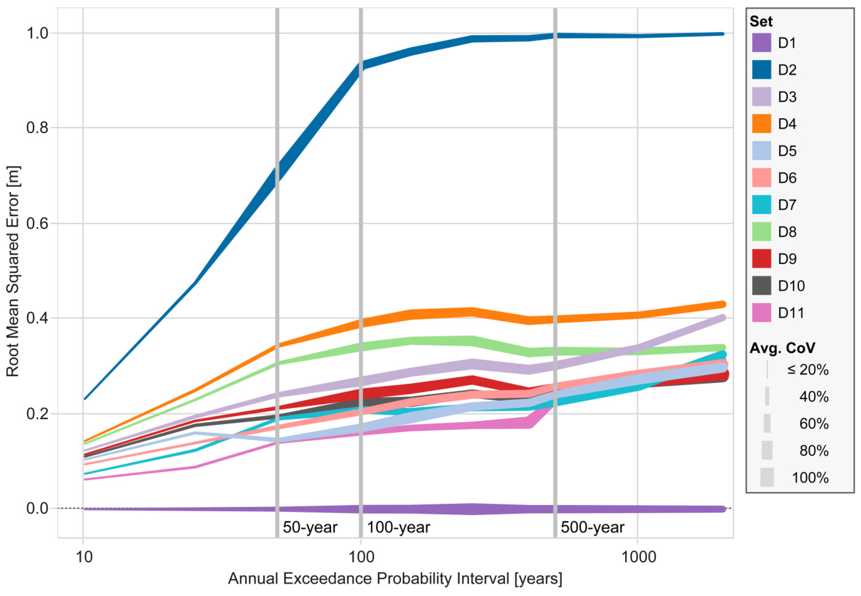
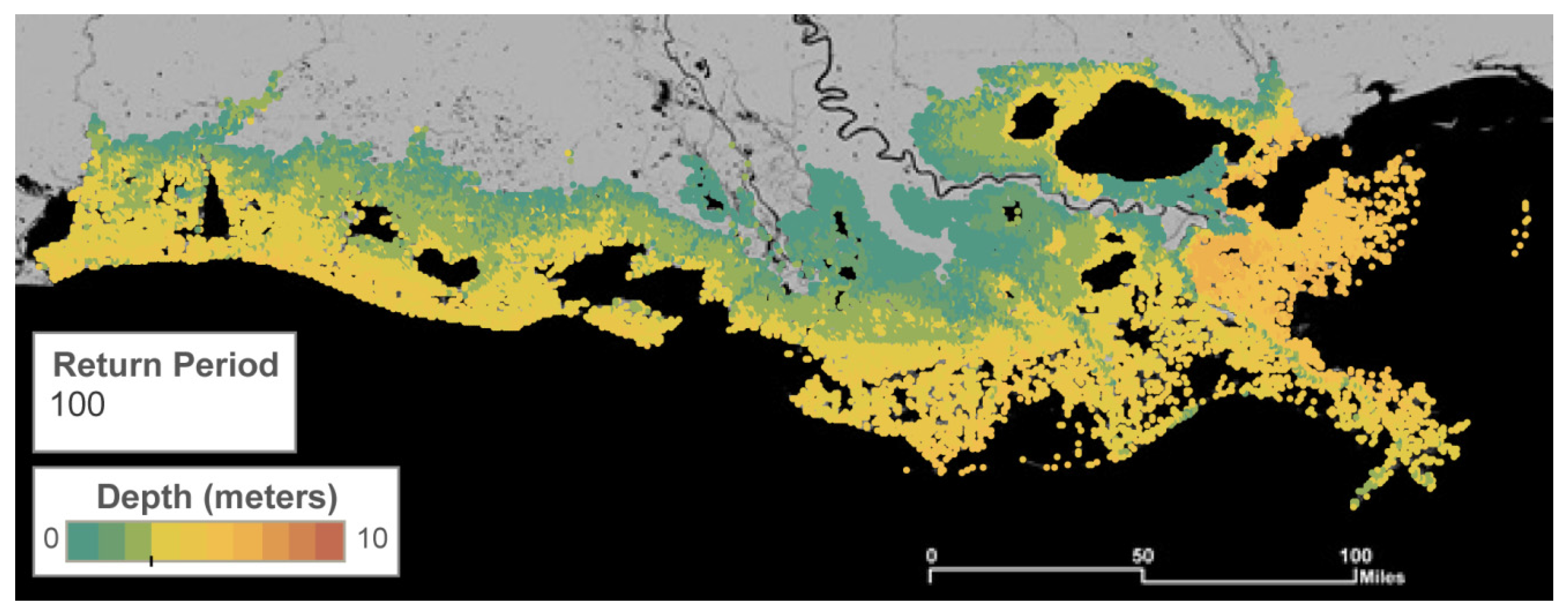
- Extract the flood depth exceedance values from the cumulative distribution functions at various return periods (A flood depth value with a (1−1/n)% annual exceedance probability (AEP)—the chance of occurring or being exceeded in a given year—is referred to as having an n-year return period. For this study, we recorded 5-, 8-, 10-, 13-, 15-, 20-, 25-, 33-, 42-, 50-, 75-, 100-, 125-, 150-, 200-, 250-, 300-, 350-, 400-, 500-, 1000-, and 2000-year exceedances.).
- Run the flood depth exceedances through CLARA’s economic module to estimate economic damage exceedances. Also estimate the expected annual damage (EAD) associated with each storm subset.
3. Experimental Section

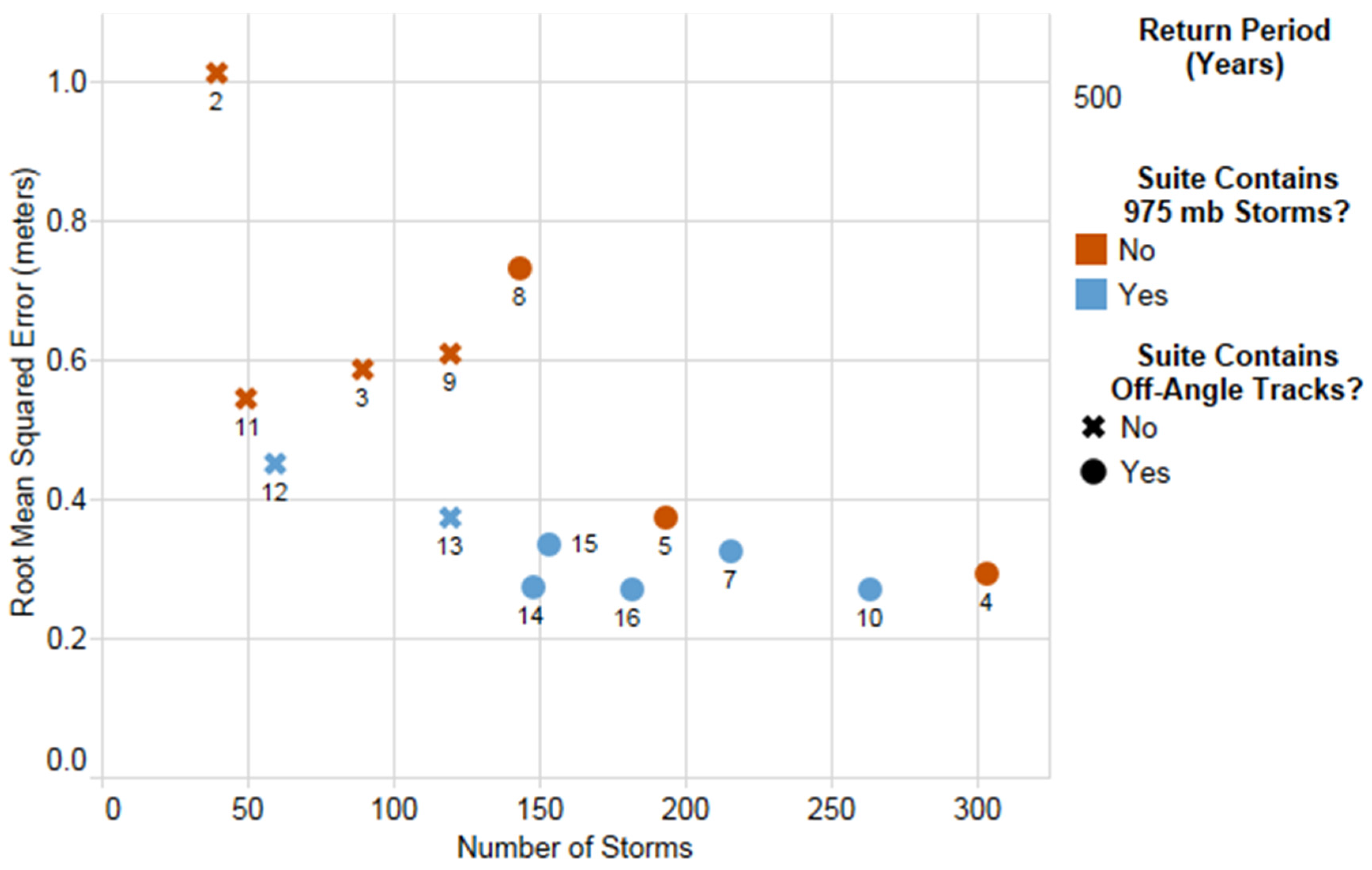
| Set | Storms | Description |
|---|---|---|
| S1 | 446 | Reference set |
| S2 | 40 | 2012 Master Plan (MP) storm suite: 10 primary storm tracks, 4 storms per track varying cp and rmax |
| S3 | 90 | 2012 MP storm suite expanded to 9 storms per track that vary cp and rmax |
| S4 | 304 | LACPR storm suite: all storms in reference set, except those with 975 mb cp |
| S5 | 194 | All storms from LACPR storm set with 11-knot vf |
| S6 | 154 | All storms from LACPR storm set with 11-knot vf on primary storm tracks |
| S7 | 216 | All storms from reference set with 11-knot vf on primary storm tracks |
| S8 | 144 | All storms from reference set on primary storm tracks with 900 mb or 930 mb cp |
| S9 | 120 | All LACPR storms on primary, central-angle tracks (includes variation in vf) |
| S10 | 264 | All storms from reference set with 11-knot vf |
| S11 | 50 | 2012 MP storm suite expanded to 5 storms per track varying cp and rmax |
| S12 | 60 | Set 11, plus storms with 975 mb cp and central values for rmax |
| S13 | 120 | All central-angle, primary-track storms with 11-knot vf (includes 975 mb storms) |
| S14 | 148 | Set 13, plus all 960 mb and 975 mb storms on secondary storm tracks |
| S15 | 154 | Set 3, plus all 960 mb and 975 mb storms on primary, off-angle storm tracks |
| S16 | 182 | Set 3, plus all 960 mb and 975 mb storms on secondary tracks or primary, off-angle tracks |
| Set | Storms | Description |
|---|---|---|
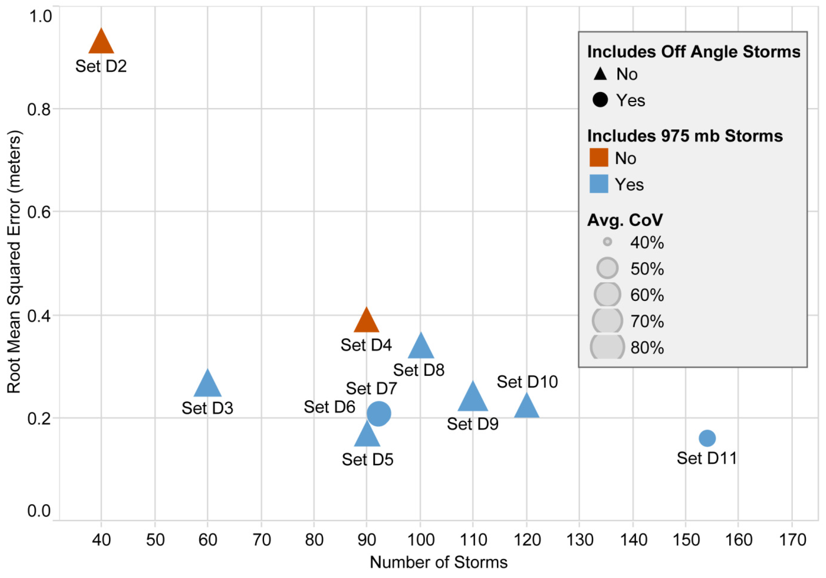
| D1 | 446 | Reference set |
| D2 | 40 | 2012 Master Plan (MP) storm suite: 10 primary storm tracks, 4 storms per track varying cp and rmax |
| D3 | 60 | 2012 MP storm suite, expanded to 5 storms per track varying cp and rmax, plus storms with 975 mb central pressure and central values for rmax |
| D4 | 90 | 2012 MP storm suite, expanded to 9 storms per track varying cp and rmax |
| D5 | 90 | 2012 MP storm suite, expanded to 7 storms per track (excludes one 930 mb and one 900 mb storm), plus 975 mb storms using extremal (rather than central) rmax values |
| D6 | 92 | Set 3, plus 960 mb and 975 mb storms on off-angle tracks only in E1-E4 |
| D7 | 92 | Set 3, plus 960 mb and 975 mb storms on off-angle tracks only in W3-W4, E1-E2 |
| D8 | 100 | All central-angle, primary-track storms with 11-knot vf, plus 975 mb storms with central rmax values |
| D9 | 110 | All central-angle, primary-track storms with 11-knot vf, plus 975 mb storms with extremal rmax values |
| D10 | 120 | All central-angle, primary track storms with 11-knot vf, including all 975 mb storms |
| D11 | 154 | Set 4, plus all 960 mb and 975 mb storms on primary, off-angle storm tracks |
4. Results and Discussion


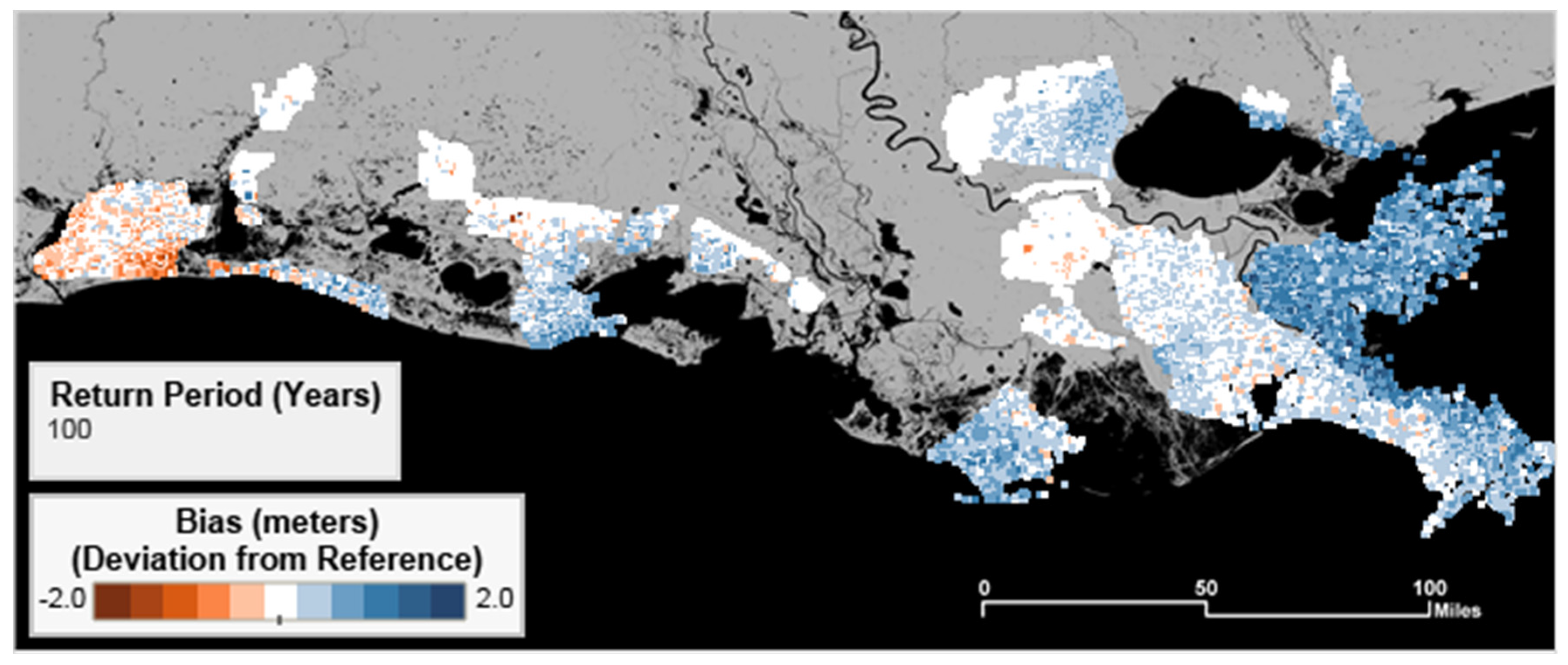
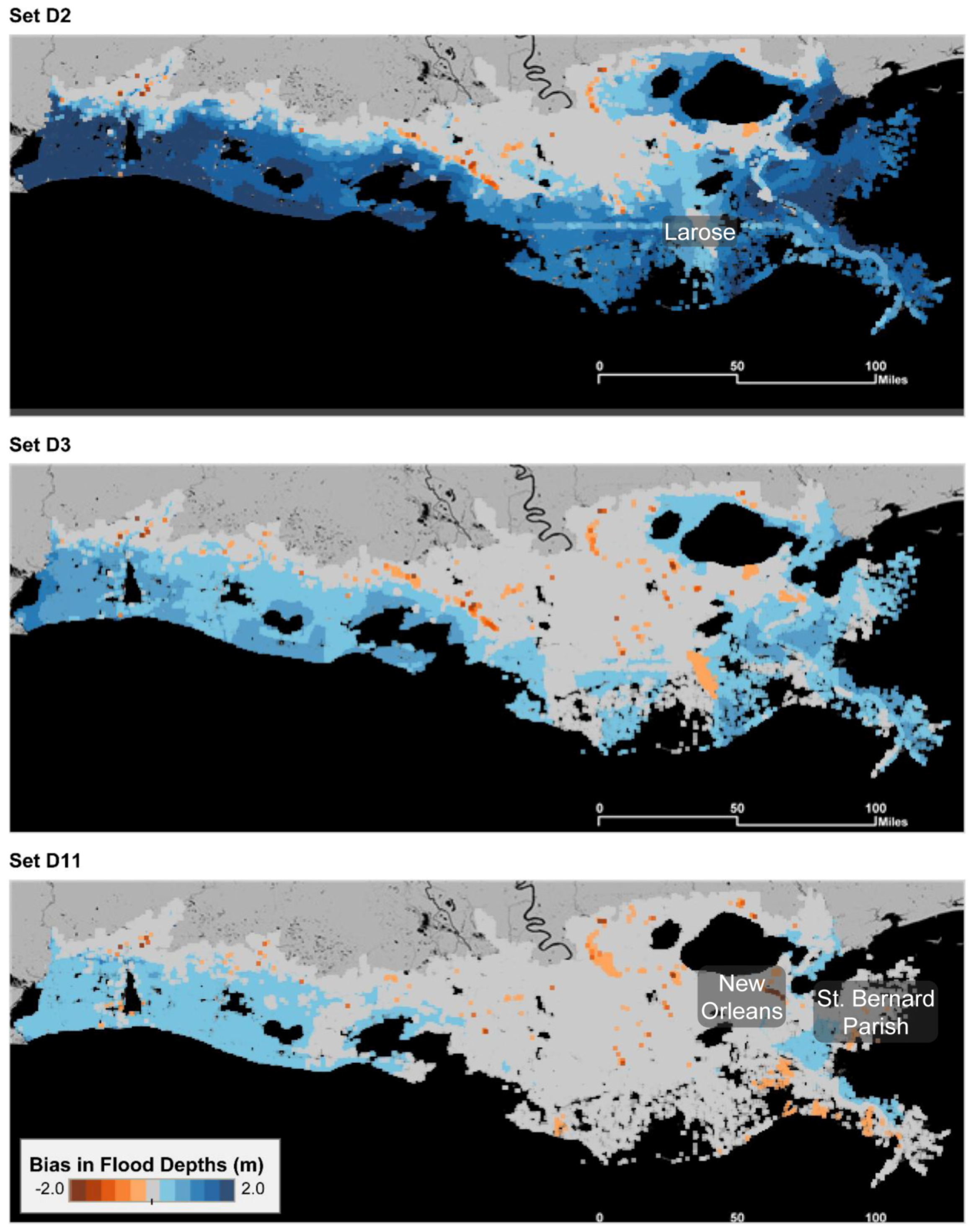
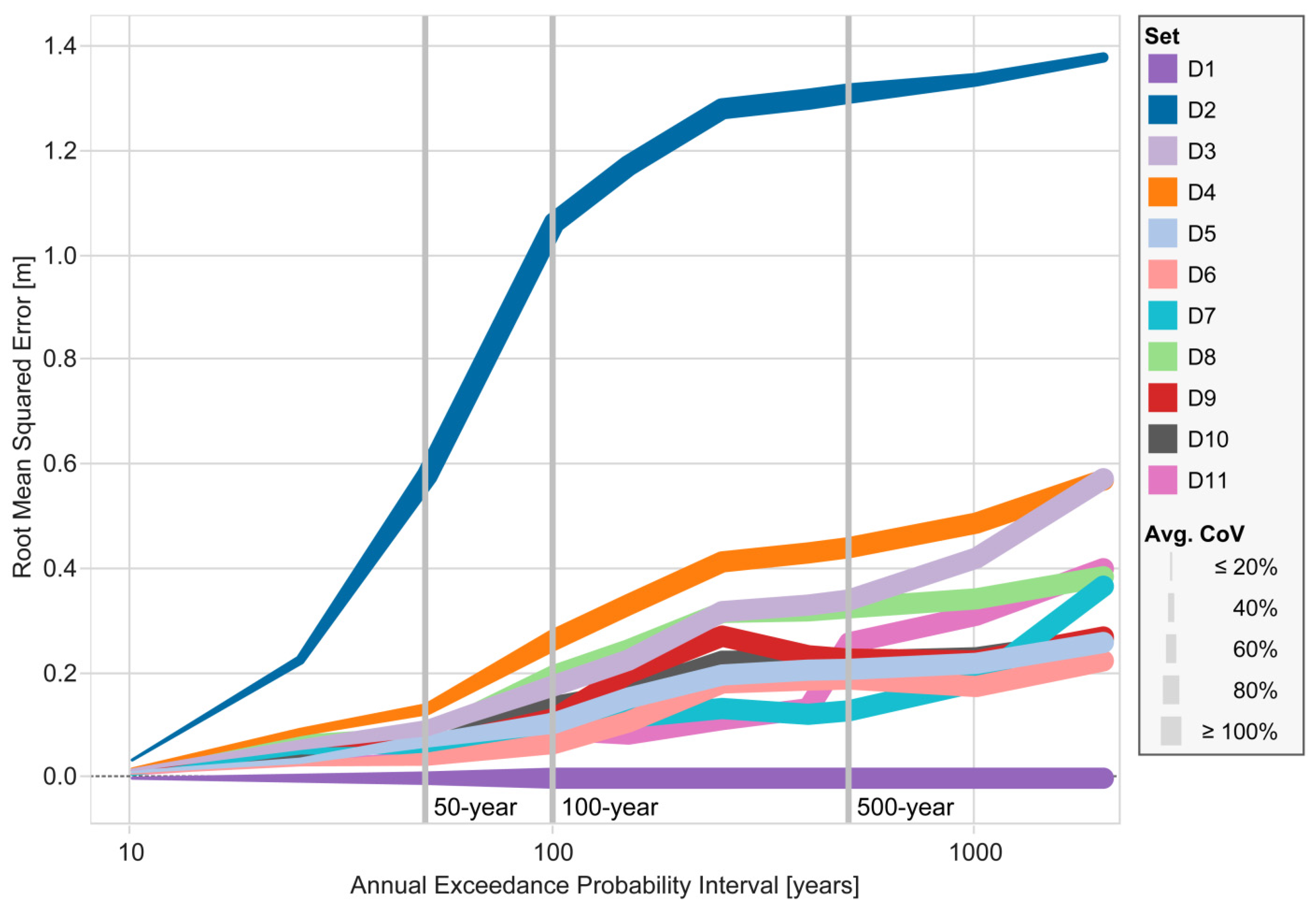
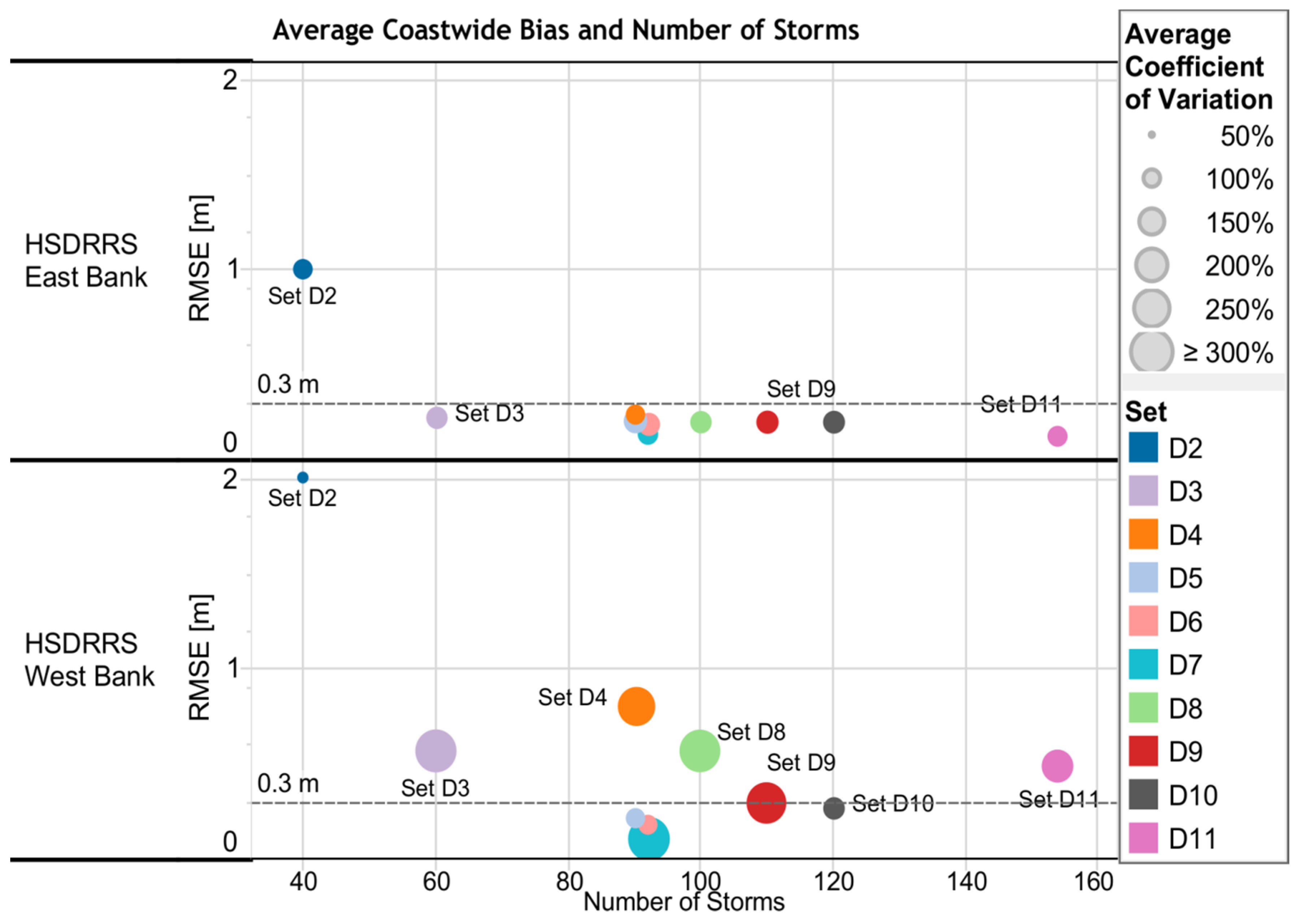
4.1. Flood Depth Bias and Variance Comparisons


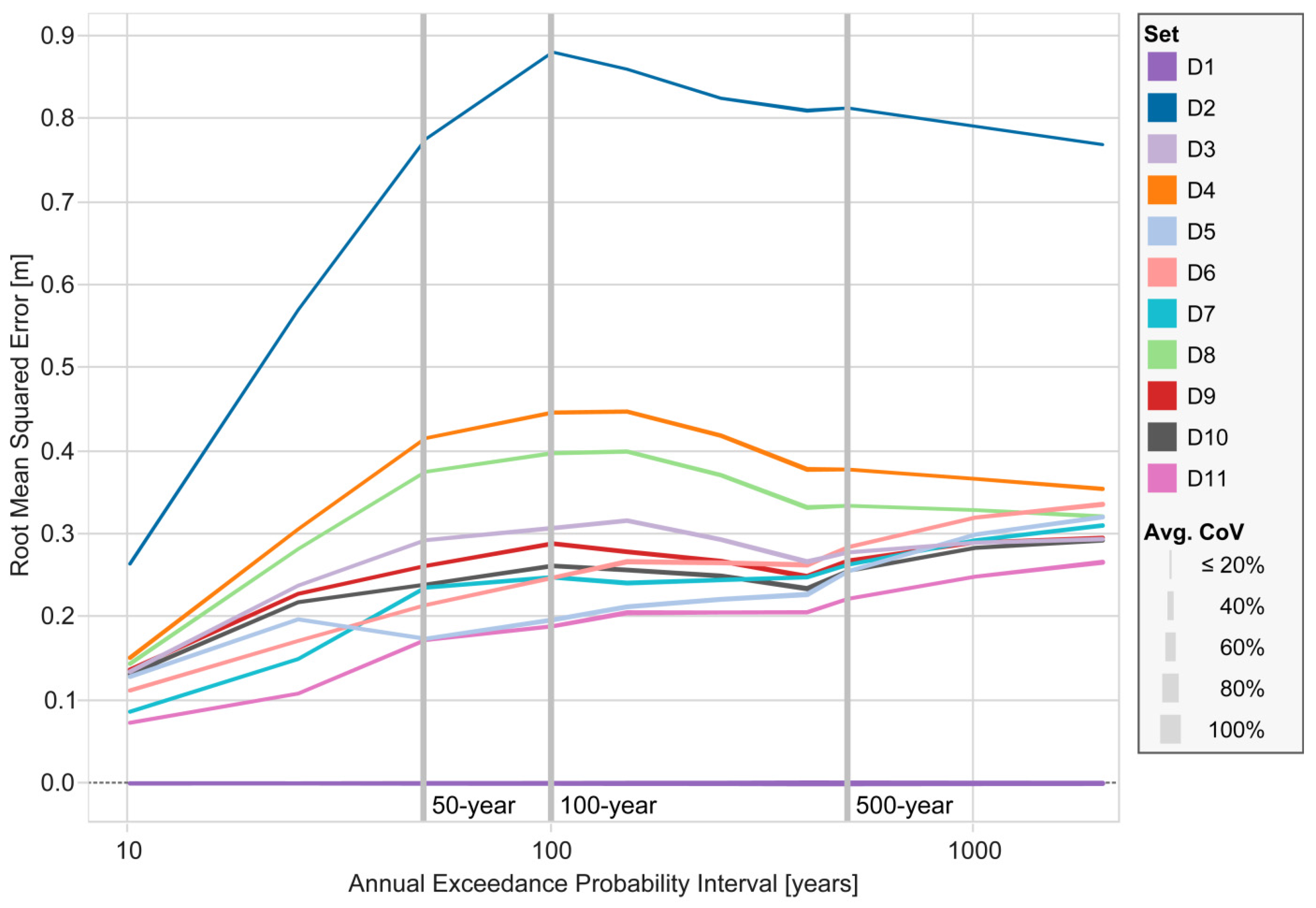
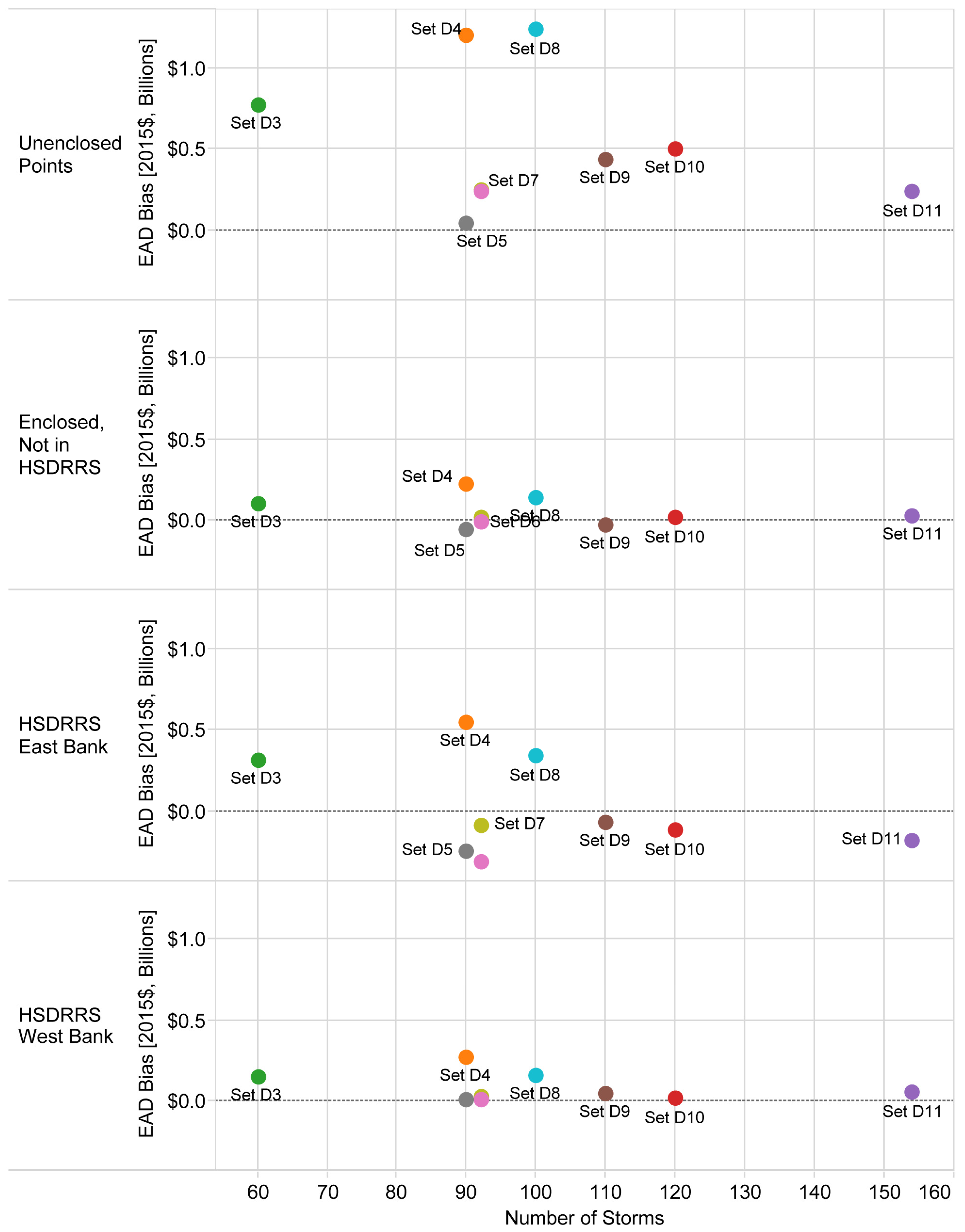
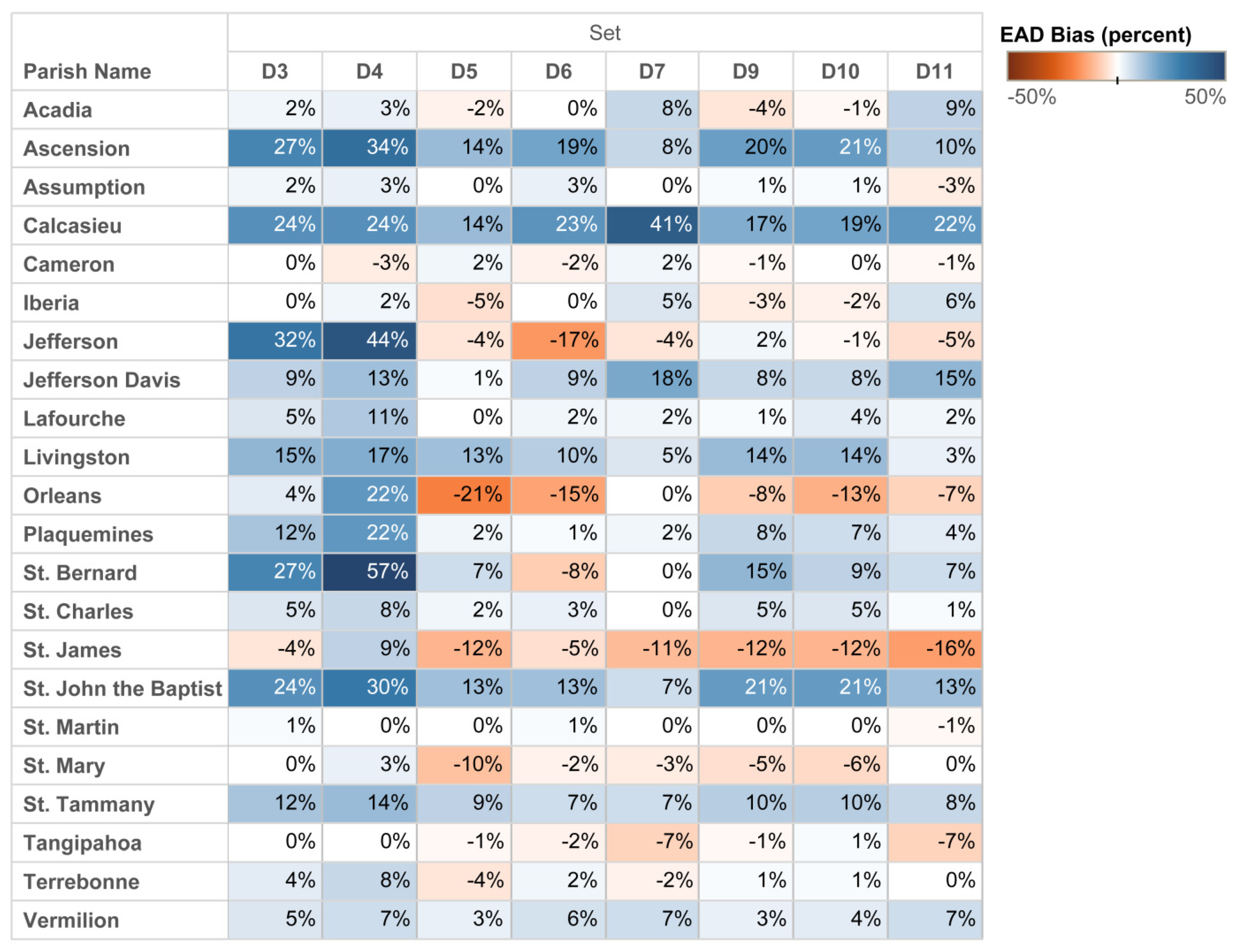
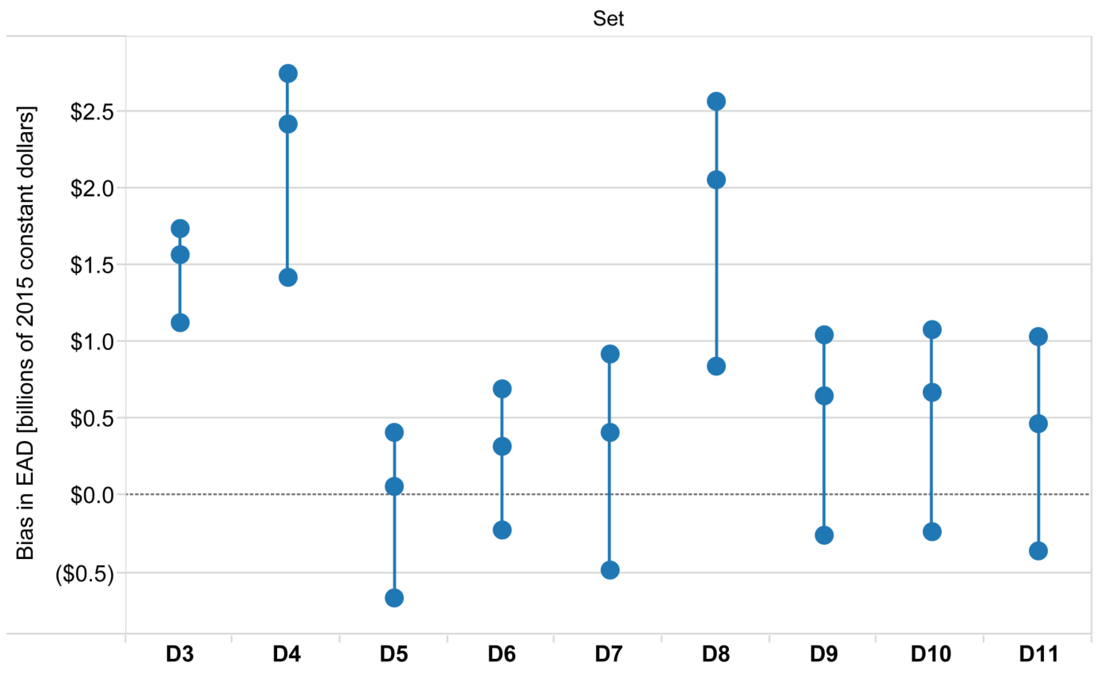
4.2. Damage Bias Comparisons


5. Conclusions
Acknowledgments
Author Contributions
Conflicts of Interest
References
- Federal Emergency Management Agency. Fact sheet: Flooding—Our nation’s most frequent and costly natural disaster. Federal Emergency Management Agency: Washington, DC, USA, 2010; p. 2. [Google Scholar]
- Karl, T.R.; Meehl, G.A.; Peterson, T.C.; Kunkel, K.E.; Gutowski, W.J., Jr.; Easterling, D.R. Weather and Climate Extremes in a Changing Climate, Regions of Focus: North America, Hawaii, Caribbean, and U.S. Pacific Islands; NOAA: Silver Spring, MD, USA, 2008.
- Burkett, V.R.; Davidson, M.A. Coastal Impacts, Adaptation and Vulnerability: A Technical Input to the 2012 National Climate Assessment; Burkett, V.R., Davidson, M.A., Eds.; Island Press: Washington, DC, USA, 2012. [Google Scholar]
- Neumann, J.E.; Emanuel, K.; Ravela, S.; Ludwig, L.; Kirshen, P.; Bosma, K.; Martinich, J. Joint effects of storm surge and sea-level rise on US coasts: New economic estimates of impacts, adaptation, and benefits of mitigation policy. Clim. Change 2014, 1–13. [Google Scholar] [CrossRef]
- Knutson, T.R.; McBride, J.L.; Chan, J.; Emanuel, K.; Holland, G.; Landsea, C.W.; Held, I.M.; Kossin, J.P.; Srivastava, A.K.; Sugi, M. Tropical cyclones and climate change. Nat. Geosci. 2010, 3, 157–163. [Google Scholar] [CrossRef] [Green Version]
- Emanuel, K. Downscaling CMIP5 climate models shows increased tropical cyclone activity over the 21st century. Proc. Natl. Acad. Sci. USA 2013, 100, 12219–12224. [Google Scholar] [CrossRef] [PubMed]
- Villarini, G.; Vecchi, G.A. Twenty-first century projections of north atlantic tropical storms from CMIP5 models. Nat. Clim. Change 2012, 604–607. [Google Scholar] [CrossRef]
- Webster, P.J.; Holland, G.J.; Curry, J.A.; Chang, H.R. Changes in tropical cyclone number, duration, and intensity in a warming environment. Science 2005, 309, 1844–1846. [Google Scholar] [CrossRef] [PubMed]
- Resio, D.T.; Irish, J.L.; Cialone, M.A. A surge response function approach to coastal hazard assessment. Part 1: Basic concepts. Nat. Hazards 2009, 51, 163–182. [Google Scholar] [CrossRef]
- Irish, J.L.; Resio, D.T.; Cialone, M.A. A surge response function approach to coastal hazard assessment. Part 2: Quantification of spatial attributes of response functions. Nat. Hazards 2009, 51, 183–205. [Google Scholar] [CrossRef]
- Toro, G.R.; Resio, D.T.; Divoky, D.; Niedoroda, A.W.; Reed, C. Efficient joint-probability methods for hurricane surge frequency analysis. Ocean Eng. 2010, 37, 125–134. [Google Scholar] [CrossRef]
- Ho, F.P.; Myers, V. Joint Probability Method of Tide Frequency Analysis Applied to Apalachicola Bay and St. George Sound, Florida; U.S. Department of Commerce: Silver Spring, MD, USA, 1975.
- Myers, V. Joint probability method of tide frequency analysis applied to Atlantic City and Long Beach Island, New Jersey; U.S. Department of Commerce: Silver Spring, MD, USA, 1970.
- Shen, W. Does the size of hurricane eye matter with its intensity? Geophys. Res. Lett. 2006, 33, L18813. [Google Scholar] [CrossRef]
- Westerink, J.J.; Luettich, R.A.; Feyen, J.C.; Atkinson, J.H.; Dawson, C.; Roberts, H.J.; Powell, M.D.; Dunion, J.P.; Kubatko, E.J.; Pourtaheri, H. A basin- to channel-scale unstructured grid hurricane storm surge model applied to southern Louisiana. Mon. Weather Rev. 2008, 136, 833–864. [Google Scholar] [CrossRef]
- Cobell, Z.; Zhao, H.; Roberts, H.J.; Clark, F.R.; Zou, S. Surge and wave modeling for the Louisiana 2012 Coastal Master Plan. J. Coast. Res. 2013, 88–108. [Google Scholar] [CrossRef]
- Luettich, R.A.; Westerink, J.J. Formulation and Numerical Implementation of the 2d/3d Adcirc Finite Element Model Version 44.Xx; R. Luettich: Chapel Hill, NC, USA, 2004. [Google Scholar]
- Fischbach, J.R.; Johnson, D.R.; Ortiz, D.S.; Bryant, B.P.; Hoover, M.; Ostwald, J. Coastal Louisiana Risk Assessment Model: Technical Description and 2012 Coastal Master Plan Analysis Results; RAND Corporation: Santa Monica, CA, USA, 2012. [Google Scholar]
- Johnson, D.R.; Fischbach, J.R. Using cost-effective and robust strategies to assess the potential for nonstructural risk reduction in coastal Louisiana. In Improving Flood Risk Estimates and Mitigation Policies in Coastal Louisiana under Deep Uncertainty; RAND Corporation: Santa Monica, CA, USA, 2013; pp. 67–101. [Google Scholar]
- Fischbach, J.R.; Johnson, D.R.; Kuhn, K.; Pollard, M.; Stelzner, C.; Costello, R.; Molina-Perez, E.; Sanchez, R.; Roberts, H.J.; Cobell, Z. 2017 Coastal Master Plan: Model Improvement Plan, Storm Surge and Risk Assessment Improvements (Subtask 4.9); Coastal Protection and Restoration Authority: Baton Rouge, LA, USA, 2015.
- Performance Evaluation of the New Orleans and Southeast Louisiana Hurricane Protection System; US Army Corps of Engineers: New Orleans, LA, USA, 2009.
- Louisiana Coastal Protection and Restoration Technical Report; US Army Corps of Engineers: New Orleans, LA, USA, 2009.
- Dietrich, J.C.; Tanaka, S.; Westerink, J.J.; Dawson, C.N.; Luettich, R.A., Jr.; Zijlema, M.; Holthuijsen, L.H.; Smith, J.M.; Westerink, L.G.; Westerink, H.J. Performance of the unstructured-mesh, SWAN+ADCIRC model in computing hurricane waves and surge. J. Sci. Comput. 2012, 52, 468–497. [Google Scholar] [CrossRef]
- Booij, N.; Holthuijsen, L.H.; Ris, R.C. The “swan” wave model for shallow water. Coast. Eng. Proc. 1996, 25. [Google Scholar] [CrossRef]
- Peyronnin, N.; Green, M.; Richards, C.P.; Owens, A.; Reed, D.; Chamberlain, J.; Groves, D.G.; Rhinehart, K.; Belhadjali, K. Louisiana’s 2012 Coastal Master Plan: Overview of a science-based and publicly-informed decision making process. J. Coast. Res. 2013, 67, 1–15. [Google Scholar] [CrossRef]
- Resio, D.T. White Paper on Estimating Hurricane Inundation Probabilities; US Army Corps of Engineers: New Orleans, LA, USA, 2007. [Google Scholar]
- Johnson, D.R.; Fischbach, J.R.; Ortiz, D.S. Estimating surge-based flood risk with the Coastal Louisiana Risk Assessment Model. J. Coast. Res. 2013, 67, 109–126. [Google Scholar] [CrossRef]
- Final Post Authorization Change Report: Morganza to the Gulf of Mexico, Louisiana; US Army Corps of Engineers: New Orleans, LA, USA, 2013.
- Johnson, D.R. Improving Flood Risk Estimates and Mitigation Policies in Coastal Louisiana under Deep Uncertainty; Pardee RAND Graduate School: Santa Monica, CA, USA, 2013. [Google Scholar]
- Holder, K. FEMA Accredits Hurricane and Storm Damage Risk Reduction System (HSDRRS); US Army Corps of Engineers: New Orleans, LA, USA, 2014. [Google Scholar]
- Johnson, D.R.; Fischbach, J.R.; Kuhn, K. Current and Future Flood Risk in Greater New Orleans; The Data Center: New Orleans, LA, USA, 2015. [Google Scholar]
© 2016 by the authors; licensee MDPI, Basel, Switzerland. This article is an open access article distributed under the terms and conditions of the Creative Commons Attribution license ( http://creativecommons.org/licenses/by/4.0/).
Share and Cite
Fischbach, J.R.; Johnson, D.R.; Kuhn, K. Bias and Efficiency Tradeoffs in the Selection of Storm Suites Used to Estimate Flood Risk. J. Mar. Sci. Eng. 2016, 4, 10. https://doi.org/10.3390/jmse4010010
Fischbach JR, Johnson DR, Kuhn K. Bias and Efficiency Tradeoffs in the Selection of Storm Suites Used to Estimate Flood Risk. Journal of Marine Science and Engineering. 2016; 4(1):10. https://doi.org/10.3390/jmse4010010
Chicago/Turabian StyleFischbach, Jordan R., David R. Johnson, and Kenneth Kuhn. 2016. "Bias and Efficiency Tradeoffs in the Selection of Storm Suites Used to Estimate Flood Risk" Journal of Marine Science and Engineering 4, no. 1: 10. https://doi.org/10.3390/jmse4010010