Multi-Fraction Bayesian Sediment Transport Model

Abstract

A Bayesian approach to sediment transport modeling can provide a strong basis for evaluating and propagating model uncertainty, which can be useful in transport applications. Previous work in developing and applying Bayesian sediment transport models used a single grain size fraction or characterized the transport of mixed-size sediment with a single characteristic grain size. Although this approach is common in sediment transport modeling, it precludes the possibility of capturing processes that cause mixed-size sediments to sort and, thereby, alter the grain size available for transport and the transport rates themselves. This paper extends development of a Bayesian transport model from one to k fractional dimensions. The model uses an existing transport function as its deterministic core and is applied to the dataset used to originally develop the function. The Bayesian multi-fraction model is able to infer the posterior distributions for essential model parameters and replicates predictive distributions of both bulk and fractional transport. Further, the inferred posterior distributions are used to evaluate parametric and other sources of variability in relations representing mixed-size interactions in the original model. Successful development of the model demonstrates that Bayesian methods can be used to provide a robust and rigorous basis for quantifying uncertainty in mixed-size sediment transport. Such a method has heretofore been unavailable and allows for the propagation of uncertainty in sediment transport applications.

1. Introduction

Sediments transported in natural systems contain a range of grain sizes. It is well understood that the transport rates of individual size fractions, when placed in a mixture, are different than when in a uni-size bed (e.g., [1,2,3]). Nonetheless, for simplicity, many transport formulas are based on an approximation that uses a single characteristic grain size (e.g., D₃₅ or D₅₀, or the grain sizes for which 35% and 50% of the particles are smaller) to represent the actual range of sizes in the sediment. Such simplifications can be useful, but cannot capture many sub-processes that drive grain sorting and can thereby influence overall transport.

A Bayesian approach to sediment transport modeling can provide a robust estimate of the predictive and parametric uncertainty that is difficult to formulate using deterministic theory or frequentist statistics [4,5]. For simplicity, previous Bayesian models have been developed using an aggregate or lumped approach to modeling the transport of single size fractions and bulk transport of multiple size fractions. This work [5] demonstrated that Bayesian statistics can successfully estimate both predictive and parametric uncertainty and can therefore be used to provide a quantitative estimate of, for example, cumulative sediment load.

The purpose of this paper is to implement a Bayesian approach for the transport of an arbitrary number of particle sizes. Such a multi-fraction model presents challenges over the previous uni-size model because the number of parameters increases directly with the number of size fractions, requiring a modification in the approach used to identify the model fit.

The Wilcock-Crowe equations [6] are used as the deterministic “center” of the model developed in this paper and the laboratory flume data that were used in their development [7] are used as a test data set. The Wilcock-Crowe equations are based on surface grain size, rather than bulk grain size that mixes surface and subsurface distributions. Hence, the transport rates are scaled to the size population immediately available for transport. This method avoids the ambiguity associated with grain sorting processes that cause a discrepancy between sediments under transport and those comprising the bulk bed mixture. Further, these equations have been used in numerous applications in the literature and in practice (for example, [8,9]), thereby making it a good candidate for use in a Bayesian framework.

1.1. Background

Previous work provides context for the motivation in developing Bayesian sediment transport models and demonstrates their utility in parameter estimation, incorporating prior knowledge, quantifying uncertainty, and in making probability-based predictions. For example, Schmelter et al. [4] modeled sediment transport in the Snake River using a bulk transport approach. Even without explicit consideration of the transport rate of different size fractions, the unit volumetric discharge of sediment was successfully modeled and this analysis was used to develop a sediment budget of the river with defined uncertainty. In systems where it is important to characterize the individual rates of movement for different size classes, this uni-size or bulk transport approach is not sufficient. For example, the Trinity River in northern California is a system that is actively being managed and “restored” after having been impacted by pervasive hydraulic and dredger mining and the construction of a large dam that diverted a large fraction of the annual runoff from the river basin. One effect of this history was an increase in fine sediments into the gravel-bedded Trinity River. Among the challenges to the Trinity River Restoration Program (TRRP), evacuation of fine sediments from the channel is a primary target, but as fine grain particles move, so do larger grains, thus quantifying the relative proportion of fine-grained to coarse-grained sediment transport becomes a relevant problem in this context. In this setting, a bulk fraction model is inadequate and a multi-fraction approach is necessary.

It is established in the literature that relative differences in grain sizes in mixed sediments results in preferential movement of specific size classes (e.g., [1,2,3,10,11]). Wilcock and Crowe [6] developed and introduced an advancement in modeling these dynamics through experimentation and the derivation of new transport equations. After making observations of multi-fraction sediment experiments in a flume, the observations were used to calibrate the transport equations and the inferred parameters were explored to develop new relationships that describe the relative size effects in mixed sediments. The research presented in this paper builds on the work of Wilcock and Crowe [6] and others [2,3] by incorporating these equations into a Bayesian model. Further, the present paper provides a formal basis for using observations to “learn” about the parameters much in the same way that Wilcock and Crowe [6] learned about the parameters through a manual calibration.

The procedure presented here provides a tool to robustly estimate model parameters (given some observations of the process) for better prediction of sediment transport rates, and for quantification of uncertainty in those predictions and in the transport model parameters. This method is offered as an alternative to manual expert calibration that relies on an individual adjusting model parameters until the model predictions are consistent with the observations. It is not the intention of this research to suggest that expert input has no place in modeling and that the purely expert-calibration is invalid. In fact, the Bayesian estimation and predictive architecture allows for incorporation of expert opinion and knowledge in ways that traditional statistical techniques do not. However, even under the assumption that Bayesian parameter estimates are no worse than the manually calibrated parameter values, the Bayesian method presents a more robust way of quantifying both parametric and predictive uncertainty compared to manual calibrations. Further, the estimated parameter values can then be used as in [6] to explore the inferred parameters and data to evaluate the extent to which the functional relationships derived in Wilcock and Crowe [6] are supported or challenged by the Bayesian estimates.

1.2. Objectives

The scope of this study includes three general objectives: (1) improve the previous Bayesian models published by Schmelter and others [4,5,12,13] extending the model from one to many fractions and by including a more suitable prior and a dimensionally scalable MCMC (Markov Chain/Monte Carlo) algorithm; (2) test the novel model using laboratory flume data and validate the Bayesian model results against previous work and other statistical methods; and (3) evaluate the model by examining differences between the Bayesian model output and the validation data analysis, by exploring what is gained by adopting a Bayesian approach over previous approaches, and developing conclusions regarding the suitability of the Bayesian multi-fraction transport model.

2. Experimental Section

2.1. Model Formulation

The proposed Bayesian model is comprised of two parts. First is the deterministic model that is assumed to generally describe the mean behavior of the phenomenon. Second is the Bayesian model into which the deterministic model is nested such that the parametric and predictive uncertainty of the deterministic equations can be estimated. The term “model” in this paper is used to describe both the sediment transport relations defined by the Wilcock-Crowe equations as well as the Bayesian statistical model. Readers are referred to [6,7] for further information on the Wilcock-Crowe equations and Schmelter et al. [5,12] for further details on Bayesian sediment transport models.

2.1.1. Sediment Transport Governing Equations

Wilcock et al. [7] performed a series of 38 sediment transport experiments in a flume 0.6 m wide and 7.9 m long supplementing 10 previous experiments for another sediment mixture, thereby totaling 48 flume runs with five sediments in which flow, transport rate, and bed surface grain size were measured over a range of different water discharges. The sediments that comprised these 48 runs varied in bulk sand content (particle sizes smaller than 2 mm), from 6% to 34%.

Nine or ten flume runs were conducted with each of five different sediment mixtures: J06 (6.2% sand), J14 (14.9%), J21 (20.6%), J27 (27.0%), and BOMC, or Bed of Many Colors (34.3%). The flume experiments themselves were brought to a steady-state condition in a water and sediment recirculating flume prior to measurement of discharge and fractional sediment transport. Wilcock and Crowe [6] utilized these data to develop a surface-based sediment transport equation that accounts for the sorting processes that result in grain hiding in mixed sediments. The transport equations, below, were calibrated by eye—that is, the model parameters (reference stress of each size fraction) were adjusted until the model fit the observations as judged by expert opinion and experience. These calibrated reference stresses were then used in subsequent analysis that explored relative size effects using a hiding function and the effect of sand content on the mobility of the entire mixture.

The Bayesian framework allows for integration of deterministic functions into a probabilistic framework [14]. Wilcock and Crowe [6] proposed a set of equations that accounts for the transport of different size fractions on the surface of a river bed and their interactions as a function of the proportion of fines contained in the bed surface. These equations are used as the deterministic function that provides the mean value of the distribution of predicted transport. Sediment transport can be described in non-dimensional terms:

$$W_j^{*}=\{\begin{array}{cc}0.002{\varphi }^{7.5}& \text{for }\varphi <1.35\\ 14{\left(1-\frac{0.894}{\sqrt{\varphi }}\right)}^{4.5}& \text{for }\varphi \ge 1.35\end{array}$$

(1)

where $W_j^{*}$ is the dimensionless transport rate of the jth size fraction, $\varphi =\tau ʹ/{\tau }_{rj}$, τ_rj is the reference stress of the jth size fraction (ML⁻¹T⁻²), and τʹ is the skin friction shear stress (ML⁻¹T⁻²). $W_j^{*}$ is defined as:

$$W_j^{*}=\frac{g{q}_{s,j}(s-1)}{F_j{u}_{*}^3}$$

(2)

where g is the acceleration due to gravity (LT⁻²), q_s,j is the unit bed load transport rate of the j^th size fraction [L²/T], s is the specific gravity (2.65), F_j is the proportion of size j on the bed surface, $u^{*}=\sqrt{\tau ʹ/\rho }$(LT⁻¹), and ρ is the density of the water (ML⁻³).

The reference stress τ_rj is a surrogate for the critical stress at initial grain motion. Equation (1) is the basis of a similarity collapse using τ_rj as the single adjustable parameter [3,15]. Equation (1) is similar in form to the equations proposed by Parker [16,17] and used in a previous Bayesian analysis by Schmelter et al. [4]. The relation can be applied to bulk transport by dropping the j subscript.

One of the key features of the multi-fraction model is the hiding function, a concept attributed to Einstein [1] that describes the effect of relative grain size on transport rate. Generally, fine grains in a mixed sediment will be shielded or hidden from the flow, thereby reducing their mobility. Coarser fractions are generally more mobile because of the smoothing effect fine grains have on the bed surface. The interaction between the jth size fraction reference shear stress and that of the geometric mean size reference shear stress was estimated in Wilcock and Crowe [6] and is defined as:

$$\frac{{\tau }_{rj}}{{\tau }_{r,sm}}={\left(\frac{D_j}{D_{sm}}\right)}^b$$

(3)

where τ_r,sm is reference shear stress for the geometric mean particle size of the surface (ML⁻¹T⁻²), D_sm is the geometric surface mean diameter (L), and the exponent b (dimensionless) in (3) is:

$$b=\frac{0.67}{1+\exp \left[1.5-\frac{D_j}{D_{sm}}\right]}$$

(4)

The remaining part of the model is prediction of τ_r,sm, which Wilcock and Crowe [6] found depended on the fraction of sand in the bed surface. It was determined that the Shields parameter, ${\tau }_{r,sm}^{*}$ (ML⁻¹T⁻²), in the sediment experiments varied with sand content, F_S, by:

$${\tau }_{r,sm}^{*}=0.021+0.015\exp [-20F_s]$$

(5)

where the conversion to dimensionless shear stress from shear stress follows:

$${\tau }_{r,sm}^{*}=\frac{{\tau }_{r,sm}}{(s-1)\rho g{D}_{sm}}$$

(6)

2.1.2. Multi-fraction Bayesian Transport Model

Using the Wilcock et al. [18] data, two Bayesian models were developed. The first model evaluates the bulk sediment transport, that is, it does not partition transport into different size fractions and therefore infers a reference stress that is representative of the mixture as a whole (bulk transport). This model is identical to that proposed in Schmelter et al. [4,12] with the exception of the specification of the prior distribution for the variance parameter and the deterministic function for the likelihood mean. The bulk transport model is described as:

$$\left[{\tau }_{r,bk},{\sigma }_{bk}^2|\log (Q_{s,o})\right]\propto {\displaystyle \prod _{i=1}^n\left[\log (Q_{s,o,i,bk})|{\tau }_{r,bk},{\sigma }_{bk}^2\right]\left[{\tau }_{r,bk}\right]\left[{\sigma }_{bk}^2\right]}$$

(7)

where τ_r,bk ~ TN(μ_bk,ψ_bk,a_bk,b_bk) is the reference shear stress of the bulk transport rate (ML⁻¹T⁻²) with hyperpriors μ_bk,ψ_bk,a_bk,b_bk; ${\sigma }_{bk}^2$ ~ N(η_bk,γ_bk²) is the variance of the bulk transport (ML⁻¹T⁻²)² with hyperpriors η_bk,γ_bk²; Q_s;o;i;bk is vector of n observations (for i = 1,...,n) of sediment transport summed across all size fractions for a given flow condition (shear stress) and Q_s,0 is the vector of sediment transport observations. The logarithm of Q_s,0 is used because transport rate is a power function of shear stress and is modeled as log(Q_s,o,i,bk) ~ N(log(Q_s,i,bk),σ_b²), where the mean value of the distribution is the logarithm of the dimensionalized transport rate (i.e., Qs rather than W*) calculated by Equations (1) and (2). This first model evaluates the total bed load transport of all size fractions for a given flow condition in aggregate and results from the likelihood and priors described immediately above.

The second model is a multi-fraction sediment transport model that distinguishes transport between one size fraction to another. This model is very similar to Equation (7) except that the joint likelihood is the product over m size fractions and n observations of each size fraction. The likelihood, or probability, is represented as:

$$\left[{\tau }_r,{\sigma }^2|\log (Q_{s,o})\right]\propto {\displaystyle \prod _{j=1}^m{\displaystyle \prod _{i=1}^n\left[\log (Q_{s,o,i,j})|{\tau }_{r,j},{\sigma }_j^2\right]\left[{\tau }_{r,j}\right]\left[{\sigma }_j^2\right]}}$$

(8)

where, Q_s,o,i,j is an n × m matrix of sediment transport observations for each size fraction (i = 1,...,n observations and j = 1,...,m size fractions). The terms in bold are vector forms of those terms defined in Equation (7) due to the use of the multiple individual particle sizes.

The likelihood, which describes the distribution from which the data are derived, has for a mean value the deterministic function of sediment transport using the Wilcock-Crowe equations:

log(Q_s,o,i,j)|τ_c,j,σ_j² ~ N(log(Q_s,i,j),σ_j²)

(9)

where Q_s,i,j is determined from Equation (1), using Equations (2)–(6). As demonstrated in previous work, the mean value of the likelihood can be any function. In the absence of a pre-defined model, the mean value of the likelihood could be a statistical function of forcing variables with unknown coefficients. In this case, the number of model parameters to estimate increases and priors would need to be specified for each of the new parameters.

The parameters to be estimated in both the bulk and multi-fraction models are the reference stress(es) and standard deviation(s). The prior reference stress for particle size j is distributed as:

τ_r,j ~ TN(μ_j,ψ_j,a_j,b_j)

(10)

where μ_j, ψ_j, a_j, and b_j are hyperpriors (mean, variance, lower support and upper support, respectively) of the truncated normal distribution on τ_r,j. For the bulk transport model, the same specification applies by simply dropping the j subscripts. The prior standard deviation for each particle size j is distributed as:

log(σ_j) ~ N(η_j,γ_j²)

(11)

where η_j and γ_j² are hyperpriors (mean and variance, respectively) of the normal distribution on log(σ_j) (essentially, a lognormal distribution on σ_j). As before, replacing the j subscript with bk specifies the prior variance for the bulk transport model.

Previous studies using a single representation fraction assumed that the Bayesian prior for the variance parameter was an inverse gamma distribution based on the required support of the random variable (positive support) as well as the fact that it was conjugate with the likelihood and made it possible to use a Gibbs sampler rather than a Metropolis-Hastings update. The initial Bayesian models described in Schmelter et al. [4,5,12] indicated that the inverse gamma, while conjugate, was not ideal for an uninformative prior. The multi-fraction model deviates from the original specification for variance distributions. Here, the log-normal prior specification for variances was explored to test alternatives to the inverse gamma.

2.2. MCMC Algorithm

The models we have used in previous Bayesian models of sediment transport (Schmelter et al. [4,5]) employed a two parameter MCMC algorithm consisting of a Gibbs sampler [19] for the variance parameter (because the prior for σ² was conjugate with the likelihood) and a Metropolis update for the reference/critical stress. The Metropolis update [20] was manually tuned. The model presented here has many more dimensions that make manually tuning the MCMC algorithm prohibitive. In previous work [4] a single tuning parameter for the critical/reference stress was all that was required to make the Markov chain converge to the target distribution. The work in this paper uses five different sediment experiments, each consisting of 13 different size fractions. Further, the modification of the prior for σ precludes the use of a Gibbs sampler because Equation (11) is not conjugate with the likelihood, therefore two Metropolis updates are required. In short, a manual tuning in the present work would require the specification of 130 tuning parameters (assuming a single chain is utilized). To avoid this, an adaptive MCMC algorithm was employed.

Adaptive MCMC algorithms essentially tune themselves such that the proposal variance (the magnitude of the random walk through the parameter space) scales are based on a pre-defined optimal acceptance ratio. There are numerous adaptive MCMC algorithms of varying complexity (e.g., [21,22,23]). For this model, a parsimonious adaptive MCMC algorithm was selected. Atchadé and Rosenthal [24] outline several adaptive algorithms and provide the framework for the algorithm used in for this model. Algorithm 4.1 of Atchadé and Rosenthal [24] was implemented for this model. This algorithm evaluates the acceptance probability and adjusts the adaptation parameter to fit a predefined optimal acceptance rate of 0.234 for this two-parameter model. Where before it was required to directly specify a tuning variance, σ², a seed tuning variance is specified that is generally appropriate and is selected by trial and error, and this initial tuning variance is adapted (modified) at each MCMC iteration such that the acceptance probability is optimal. The adapted tuning variance is defined as:

$${\sigma }_{k+1}={\sigma }_k+{\gamma }_k\left(\alpha \left(X_k, Y_{k+1}\right)-\overline{\tau }\right)$$

(12)

where γ_k = σ_k/k and effectively scales the adaptation such that with each iteration the tuning variance adapts less and less, $\alpha (x,y)=\min \left(1,\frac{\pi (y)}{\pi (x)}\right)$ π(x) is the likelihood of parameter value x, X_k is the Markov chain for the parameter of interest, Y_k+1 is a new proposal Y_k+1 ~ N(X_k,σ_k²), and $\overline{\tau }\equiv 0.234$. A random variable U ~ Uniform(0,1) is sampled, and the newly proposed value is accepted when $U\le \alpha \left(X_k,Y_{k+1}\right)$ and rejected otherwise in which case X_k+1 = X_k.

For the simulations in this research a single MCMC chain was used rather than multiple chains primarily due to the simple nature of the model itself. There are very few parameters being estimated here compared to more complex hierarchical models (we only hold interest in the reference stress and the variance parameters, rather than lower level hyper-parameters, such as the mean value of the prior distribution for the model variance) and during model fitting an ad hoc analysis of the impact of seed values for the MCMC chains was performed. This ad hoc analysis demonstrated that convergence on the target distribution was not affected by the selection of the seed value—all simulations using different seed values had converged to the same distribution. The well-behaved nature of the MCMC simulations in this research is likely due to the simple model formulation; more complicated models (higher number of parameters, inference at multiple hierarchies) will likely require more formal methods and tests to ensure validity of the posterior distribution.

3. Results and Discussion

3.1. Results

The purpose of this paper is to develop and test a Bayesian multi-fraction model centered on the Wilcock-Crowe equations using the laboratory flume data used to originally develop those equations. Using these data provides a convenient way to evaluate the inferred reference stresses from the Bayesian model as well as compare the resulting relationships of reference stress to sand content and the hiding function proposed by Wilcock and Crowe [6].

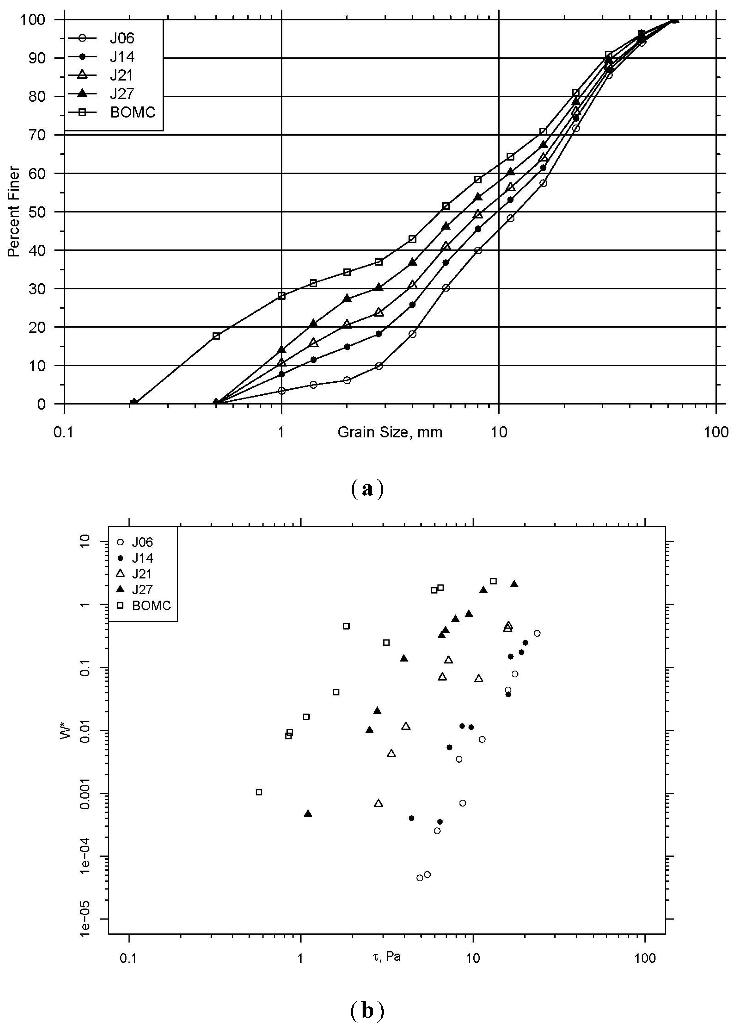
The results that follow are in three sections. The first briefly describes the dataset and provides visualizations and analysis. These also serve as illustrations of the data. The remaining two sections describe the results of the bulk and fractional transport models.

3.1.1. Experimental Data

The Wilcock-Kenworthy-Crowe (WKC) [7] data used in this research were downloaded from the original paper’s FTP site hosted by the American Geophysical Union (AGU). Several plots of the data were created for comparison against published figures for verification. Figure 1a,b are two figures that were created independently according to published data from the original paper.

Figure 1a shows the particle size distributions for each sediment mixture, which is labeled in the legend. Each sediment uses the same gravel (>2 mm) size distribution and different proportions of sand. The minimum size for the sand fraction is 0.5 mm for all sediments except BOMC, for which the minimum is 0.21 mm). The bulk transport rates of the sandier mixtures are much larger than the less sand mixtures.

Figure 1. (a) Grain-size distribution of sediments and (b) bulk transport rates from the Wilcock et al. [18] experiments (W* is defined in Equations (1) and (2)).

Figure 1. (a) Grain-size distribution of sediments and (b) bulk transport rates from the Wilcock et al. [18] experiments (W* is defined in Equations (1) and (2)).

3.1.2. Bulk Transport

The bulk transport model fitted to the observations is similar to the analysis performed in previous work (Schmelter et al. [4,12] for a single sediment size, in which a multi-fraction sediment mixture is modeled using a single fraction model. The total transport rate, integrated across all grain sizes, is the observation and prediction in such an analysis. The reference shear stress and variance inferred from this model represent the integrated or bulk behavior of the sediment mixture as an ensemble. Each different sediment mixture was analyzed in the model described by Equation (7). The inferred reference stresses and variances are summarized in Table 1.

Table 1. Data summary for sediment mixtures. Inferred bulk transport posterior means for τ_r, in Pa and σ in m³/m/s, number of observational runs for each sediment, and the proportion sand in both the surface and total mixture.

Parameter	Sediment Mixture
	J06	J14	J21	J27	BOMC
τ	8.90	7.14	3.46	1.82	0.73
σ	0.74	1.26	1.23	1.11	1.04
Observations	10	9	8	10	10
Surface sand proportion	0.0013	0.0130	0.0728	0.1990	0.4789
Total sand proportion	0.0612	0.1484	0.2056	0.2730	0.3432

Table 1. Data summary for sediment mixtures. Inferred bulk transport posterior means for τ_r, in Pa and σ in m³/m/s, number of observational runs for each sediment, and the proportion sand in both the surface and total mixture.

Parameter	Sediment Mixture
	J06	J14	J21	J27	BOMC
τ	8.90	7.14	3.46	1.82	0.73
σ	0.74	1.26	1.23	1.11	1.04
Observations	10	9	8	10	10
Surface sand proportion	0.0013	0.0130	0.0728	0.1990	0.4789
Total sand proportion	0.0612	0.1484	0.2056	0.2730	0.3432

Typical prior parameterizations for reference stress and standard deviation parameters in the likelihood of both the bulk and fractional transport models are generally vague and were used in all models.

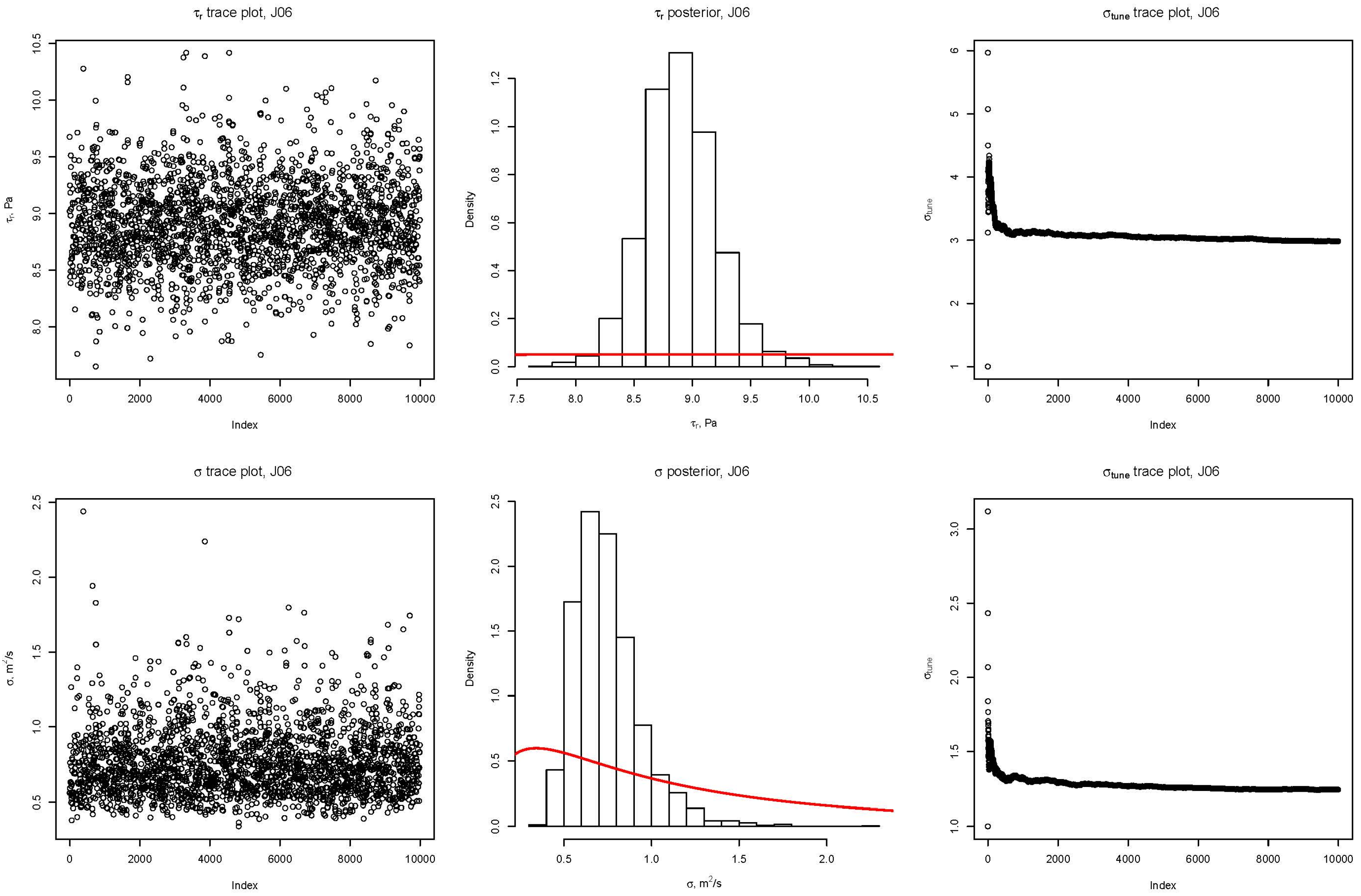
Figure 2. Trace plots for J06 sediment. Results are representative of all bulk sediments. Red line represents the prior distribution used in the model.

Figure 2. Trace plots for J06 sediment. Results are representative of all bulk sediments. Red line represents the prior distribution used in the model.

Figure 2 displays the diagnostic plots that resulted from the bulk transport model run for the J06 sediment. The left-most column shows the MCMC trace plots up to the maximum value of 10,000 samples. In these columns we see good mixing of the chains. Further, convergence was rapid and there appears to be minimal autocorrelation among the data points (partial autocorrelation plots were created and inspected, but are not included here), another indicator of valid MCMC results. The middle column shows the posterior histograms after discarding the first 2000 samples as “burn-in”. The right-most column shows the tuning variance adaptation trace plot. There are large fluctuations in the trace plot followed quickly by convergence to a stable tuning variance value. Trace plots for additional sediment exhibited similar characteristics, but are not included here.

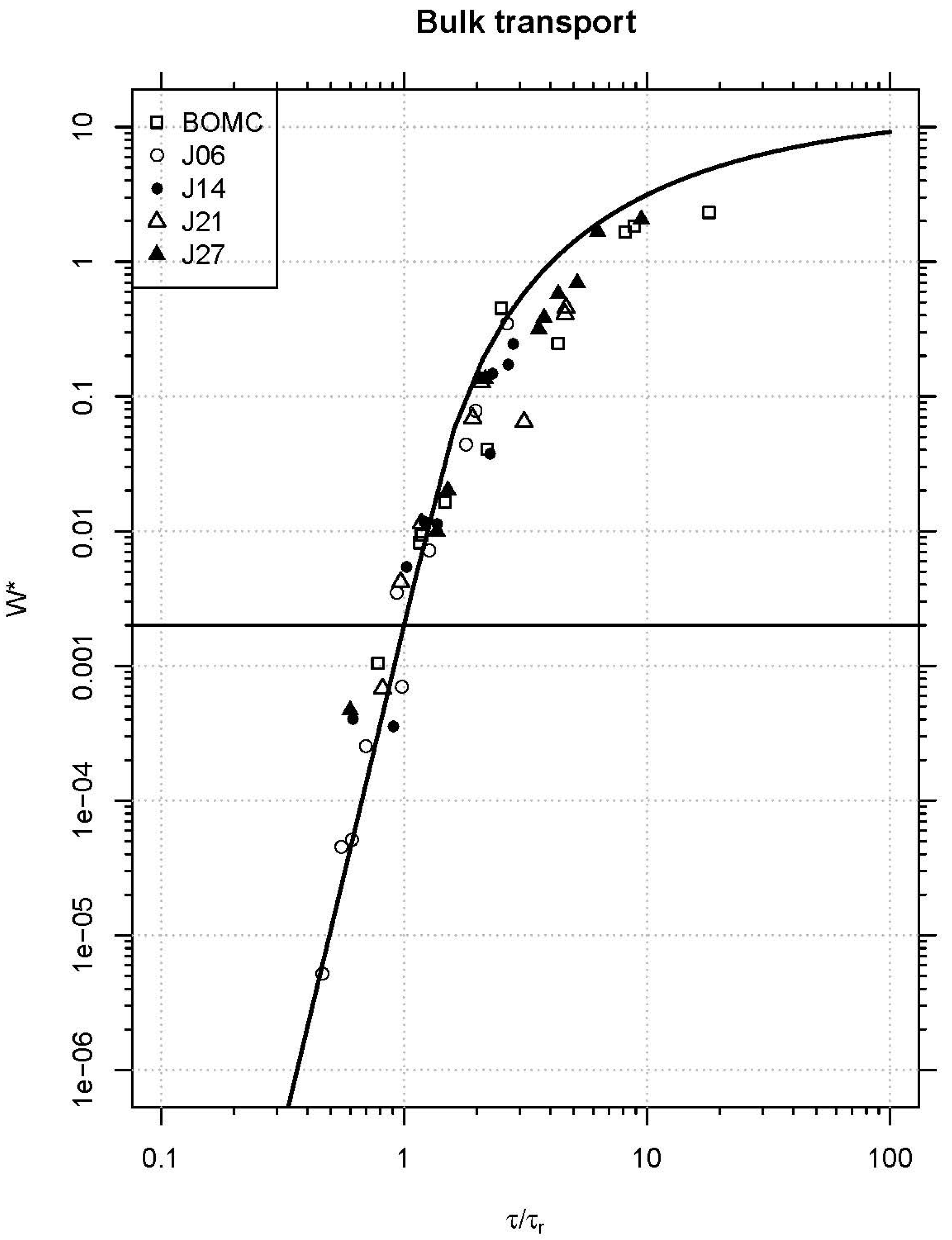
Figure 3 shows the similarity collapse of the bulk transport data. If a single transport function applies to all mixtures, then dividing each stress by the reference stress should collapse all transport observations about a common trend. The similarity collapse relies on the inferred reference stresses for each bulk sediment mixture, which are included in Table 1 along with the inferred variances and number of observations for each sediment. The mean inferred reference stresses provides the normalizing constant to make all the transport observations collapse into a single series of points. The resulting similarity collapse for the bulk transport model demonstrates that when each sediment mixture and transport observation is scaled by the inferred reference stress, then all of the points collapse into a single relationship. The line in Figure 3 (the calibrated Wilcock-Crowe Equation (1) for the bulk transport data) fits the data very well for W* values less than 0.01. Transport rates appear to be over predicted for W* values greater than 0.03, indicating a model deficiency in the case of bulk sediment transport.

Figure 3. Similarity collapse for bulk transport rates. The bold line is the calibrated Wilcock-Crowe Equation (1) for the bulk transport data. W* = 0.002 is the reference value that corresponds to the reference shear stress τ_r.

Figure 3. Similarity collapse for bulk transport rates. The bold line is the calibrated Wilcock-Crowe Equation (1) for the bulk transport data. W* = 0.002 is the reference value that corresponds to the reference shear stress τ_r.

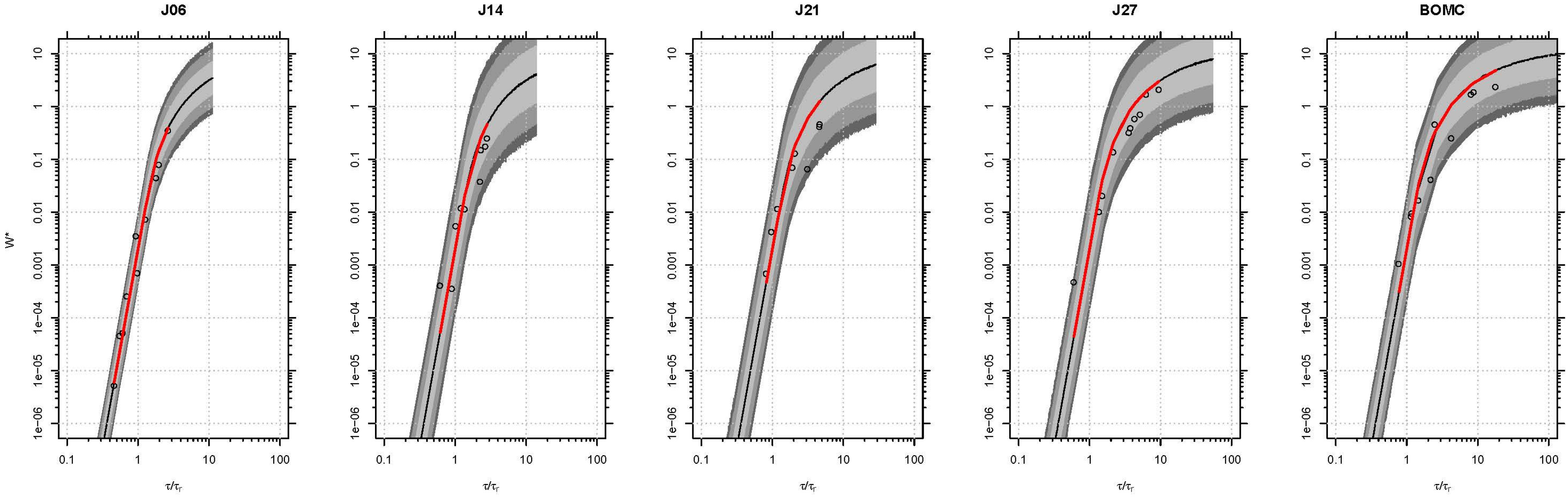
Individual posterior predictive distributions (PPDs) were calculated for each sediment mixture, and these PPDs are included as Figure 4. As a validation/check of Bayesian parameter estimates, a non-linear least squares regression was fitted to the observed data, and the resulting rating curves are represented by the red lines. This overlay demonstrates that parameter inference resulting from the Bayesian and nonlinear least squares (NLS) approaches agree, so this serves as a type of validation that the Bayesian model was correctly implemented in the code. Figure 4 also illustrates one of the primary differences defined in the Bayesian approach. Individually, the transport rating curves may also suggest systematic over-prediction evidenced by the individual rating curves for J21 and J27, though it is less convincing than the evidence provided by the similarity collapse in Figure 3.

Figure 4. Bulk rating curves. Red line shows the NLS prediction. Color coded darkest to lightest for the 95%, 90%, and 68% credible intervals.

Figure 4. Bulk rating curves. Red line shows the NLS prediction. Color coded darkest to lightest for the 95%, 90%, and 68% credible intervals.

3.1.3. Fractional Transport

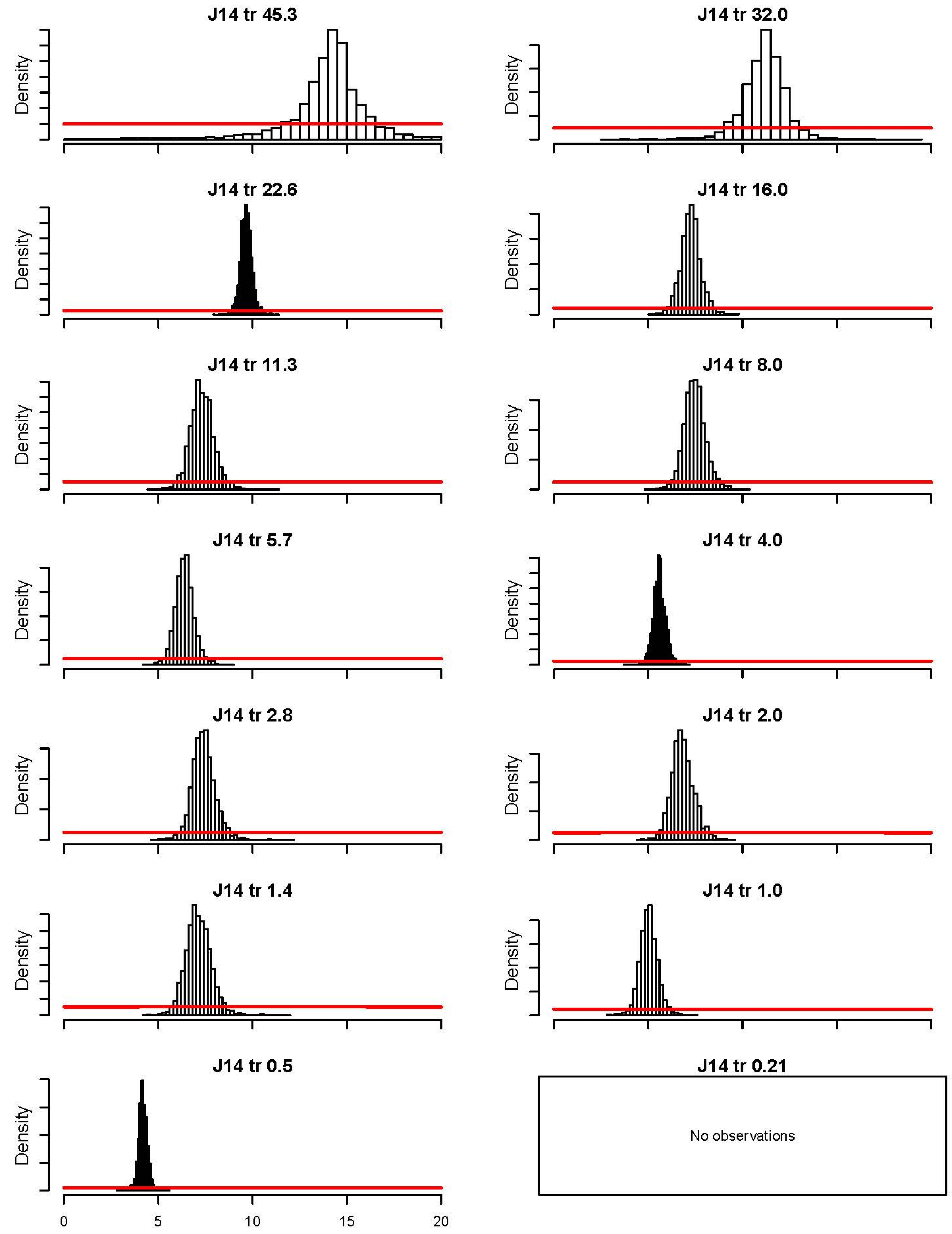
Figure 5 and Figure 6 show the posterior distributions for the fractional model fitted to the J14 sediment mixture. The distributions are plotted by size fraction, along with the prior distribution plotted as a solid (red) line for reference. Compared to the prior information supplied, which was a uniform distribution over the interval (0,20], the information provided by the observations, even where there were very few observations as is the case for the coarser grain sizes, such as 45.3 mm, (Table 2) indicates that there is still significant learning about the reference stress. One weakness of the current model, however, is that flume experiments that did not result in any movement of a particular grain size (e.g., larger grains at small τ) are not accounted for in the model. That is, only those instances where sediment moved are considered a data point, even though there is important information contained in experiments with nonmoving fractions. The current model does not use any of the information contained in zero-transport experimental runs. This is possible by specifying a lower limit in the prior distribution based on the experimental runs with no transport for some fractions. Those conditions produce a shear stress that is necessarily smaller than the reference stress for immobile fractions. Finally, incorporating this information into the model in a more formal way (i.e., developing a model that accounts for zero transport events) would be a valuable improvement in future research.

Figure 5. Fractional posterior distributions of τ_r;j for J14. Red line represents the prior distribution used in the model.

Figure 5. Fractional posterior distributions of τ_r;j for J14. Red line represents the prior distribution used in the model.

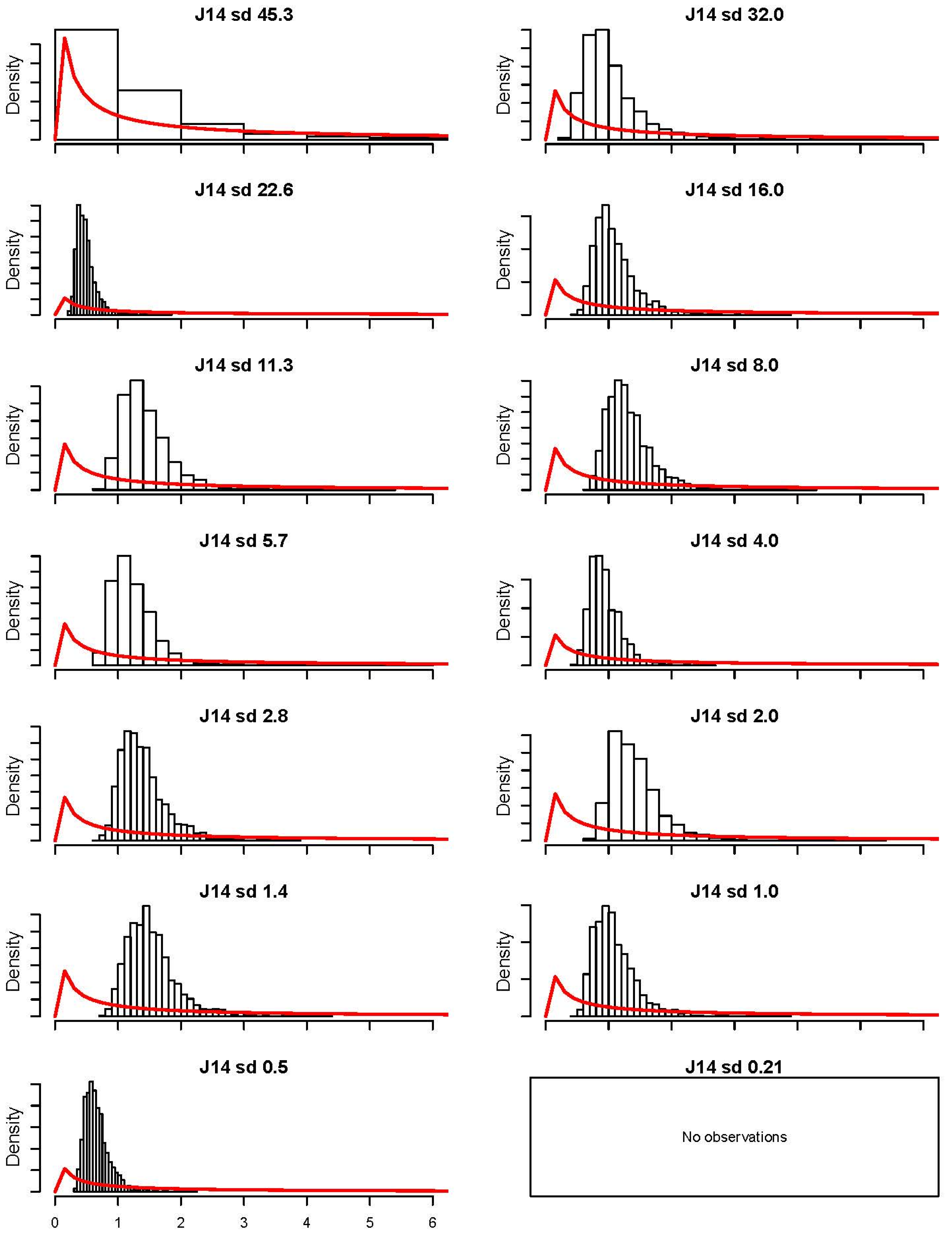
Figure 6. Fractional posterior distributions of σ_j for J14. Red line represents the prior distribution used in the model.

Figure 6. Fractional posterior distributions of σ_j for J14. Red line represents the prior distribution used in the model.

Table 2. Inferred fractional transport posterior means for τ_r,j (Pa).

Size (mm)	Sediment Mixture
	J06		J14		J21		J27		BOMC
	τr,j (Pa)	# Obs.	τr,j (Pa)	# Obs.	τr,j (Pa)	# Obs.	τr,j (Pa)	# Obs.	τr,j (Pa)	# Obs.
45.3	14.40	3	13.87	2	13.13	1	8.14	1	8.42	1
32.0	11.33	4	11.15	4	7.45	2	7.00	4	7.07	2
22.6	10.27	6	9.67	7	7.48	5	5.38	6	3.59	4
16.0	9.08	7	7.25	8	5.39	6	3.57	6	3.86	4
11.3	9.39	7	7.31	9	4.80	6	3.08	7	3.46	4
8.0	8.65	9	7.46	9	4.04	8	2.83	9	2.31	5
5.7	7.90	10	6.38	9	3.09	8	2.19	9	1.94	6
4.0	7.71	10	5.60	9	2.87	8	1.48	10	1.79	6
2.8	8.99	10	7.41	9	3.47	8	1.97	10	1.31	8
2.0	8.96	9	6.83	9	3.07	8	1.51	10	1.03	9
1.4	9.53	8	7.12	9	3.21	8	1.56	10	1.01	10
1.0	na	0	5.02	8	2.57	8	1.35	10	0.74	10
0.5	6.77	4	4.18	8	2.63	8	1.43	10	0.61	10
0.21	na	0	na	0	na	0	na	0	0.62	10

Table 2. Inferred fractional transport posterior means for τ_r,j (Pa).

Size (mm)	Sediment Mixture
	J06		J14		J21		J27		BOMC
	τr,j (Pa)	# Obs.	τr,j (Pa)	# Obs.	τr,j (Pa)	# Obs.	τr,j (Pa)	# Obs.	τr,j (Pa)	# Obs.
45.3	14.40	3	13.87	2	13.13	1	8.14	1	8.42	1
32.0	11.33	4	11.15	4	7.45	2	7.00	4	7.07	2
22.6	10.27	6	9.67	7	7.48	5	5.38	6	3.59	4
16.0	9.08	7	7.25	8	5.39	6	3.57	6	3.86	4
11.3	9.39	7	7.31	9	4.80	6	3.08	7	3.46	4
8.0	8.65	9	7.46	9	4.04	8	2.83	9	2.31	5
5.7	7.90	10	6.38	9	3.09	8	2.19	9	1.94	6
4.0	7.71	10	5.60	9	2.87	8	1.48	10	1.79	6
2.8	8.99	10	7.41	9	3.47	8	1.97	10	1.31	8
2.0	8.96	9	6.83	9	3.07	8	1.51	10	1.03	9
1.4	9.53	8	7.12	9	3.21	8	1.56	10	1.01	10
1.0	na	0	5.02	8	2.57	8	1.35	10	0.74	10
0.5	6.77	4	4.18	8	2.63	8	1.43	10	0.61	10
0.21	na	0	na	0	na	0	na	0	0.62	10

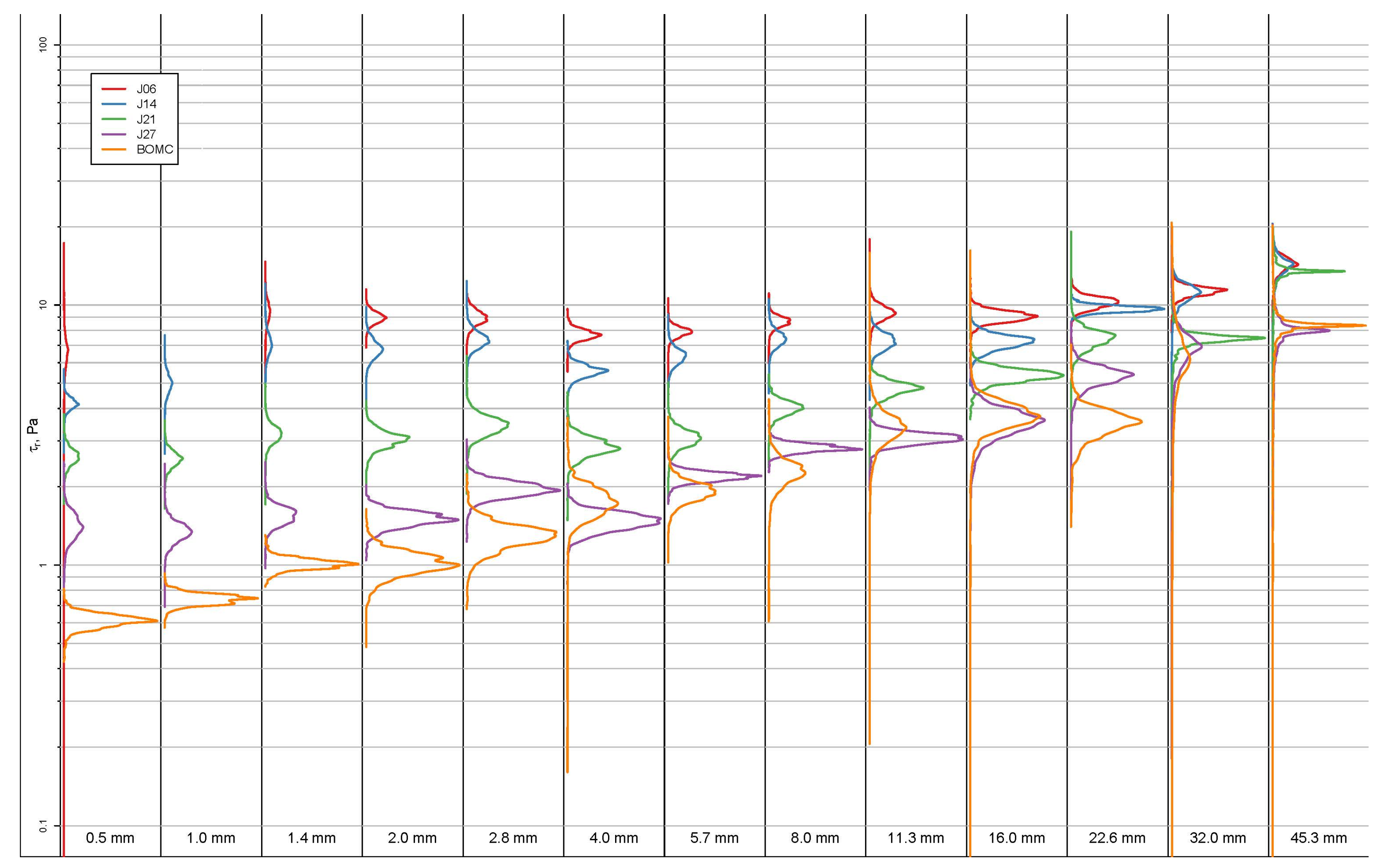
The original derivation of the Wilcock-Crowe equations was based on reference stress values that were fitted by eye in Wilcock and Crowe [6] because it was observed that optimized solutions for the parameters did not provide as good a fit visually and seemed to be overly influenced by outliers. The Bayesian model produces estimates of reference shear. The point values (means) are shown in Table 2, and the graphical representation of the posteriors is shown in Figure 7. From these densities, the inference can be visualized in a number of ways. 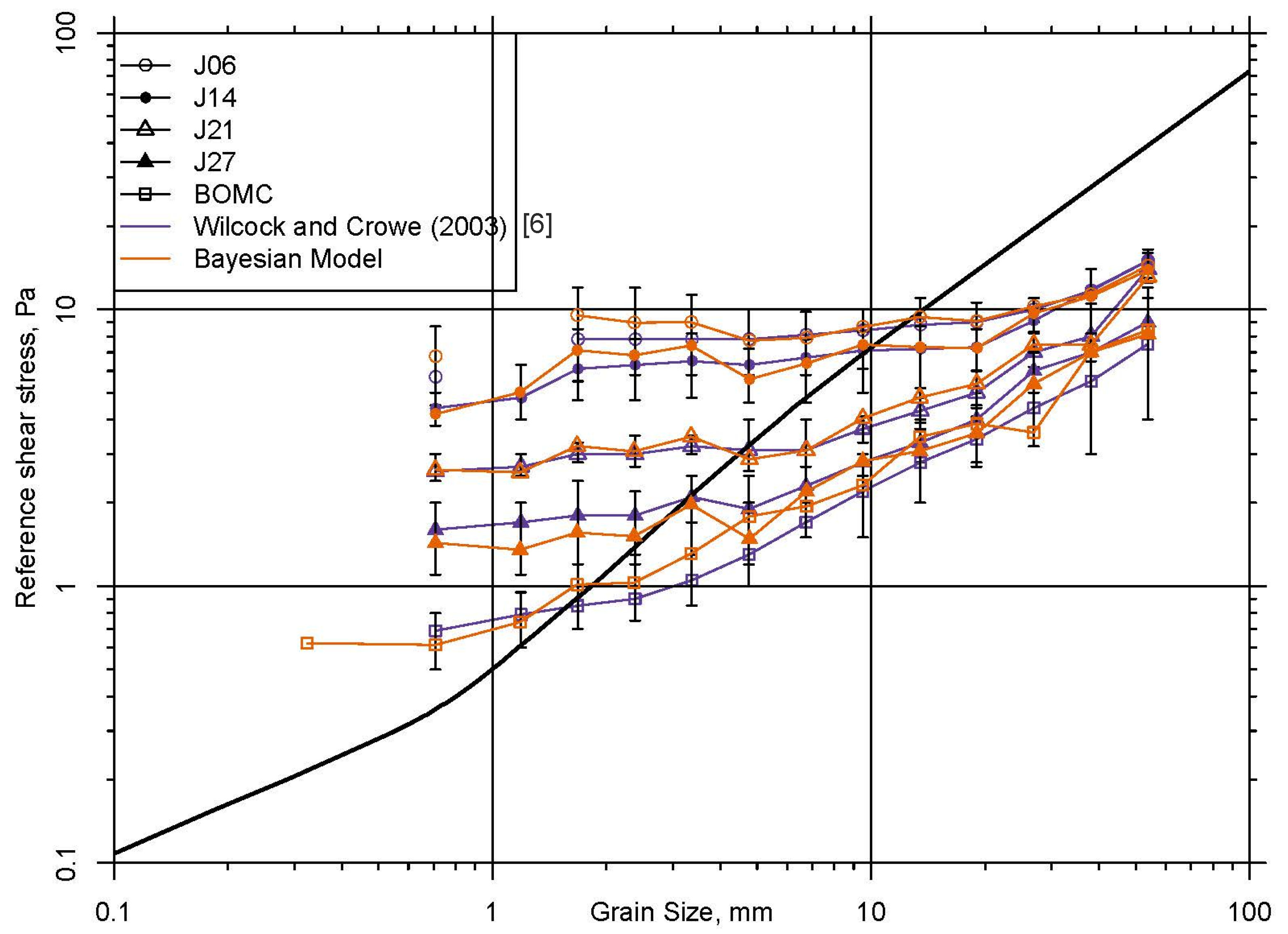Figure 8 shows the original Wilcock and Crowe [6] point estimates for reference stress, as well as error bars for each point value, along with the posterior mean values referenced in Table 2.

Figure 7. Inferred densities for reference shear stress.

Figure 7. Inferred densities for reference shear stress.

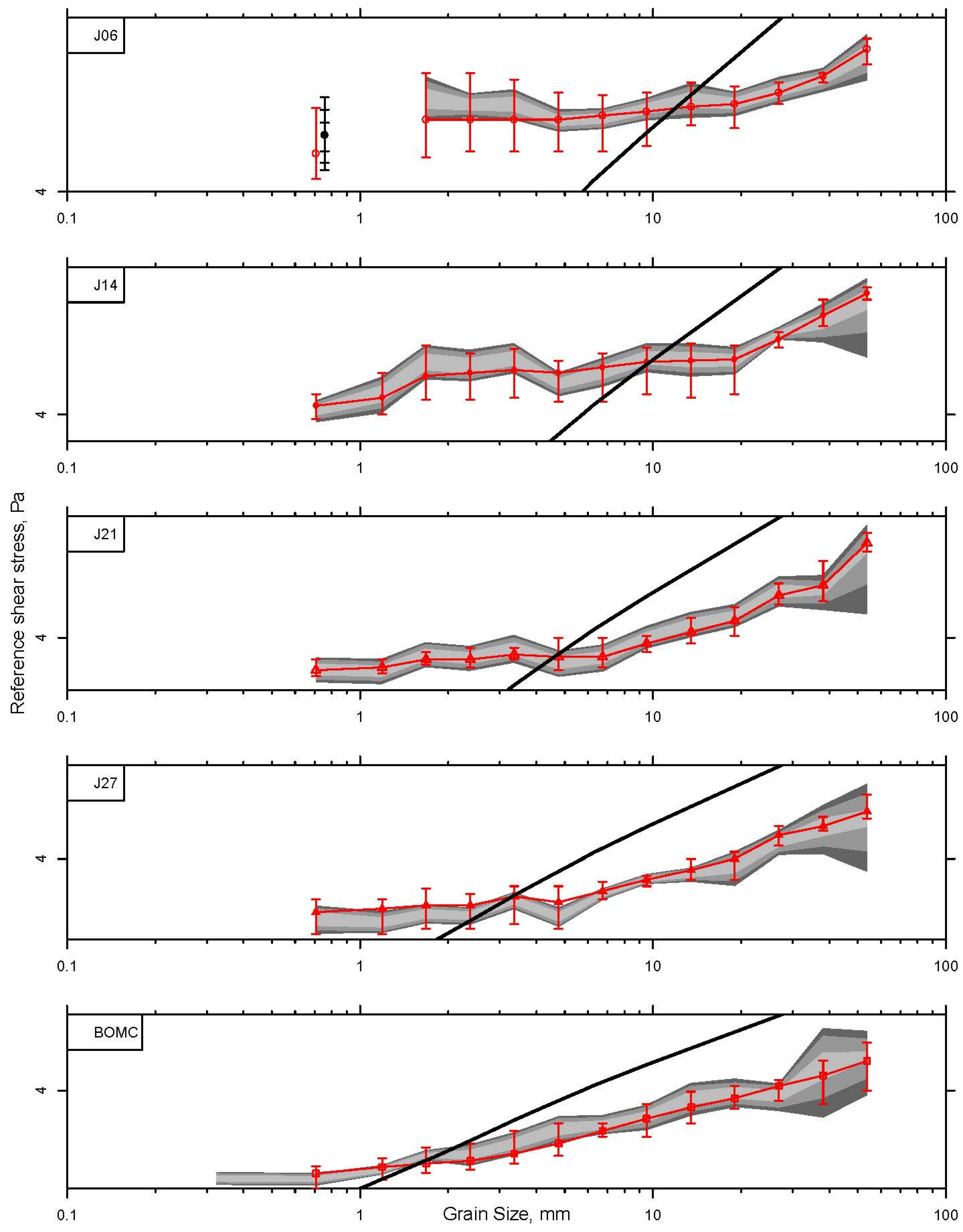
Figure 8. Comparison of original reference stress curves from Wilcock and Crowe [6] to inferred curves from Bayesian model. Error bars are those from [6]. The solid black line shows the standard Shields Curve for incipient motion of uni-size sediment.

Figure 8. Comparison of original reference stress curves from Wilcock and Crowe [6] to inferred curves from Bayesian model. Error bars are those from [6]. The solid black line shows the standard Shields Curve for incipient motion of uni-size sediment.

Reference shear stress are more widely separated among the mixtures for finer grain sizes. The mixtures with less sand are generally flatter, indicating a condition of equal mobility in which all particles begin to move at the same shear stress. Sandier mixtures exhibit a larger variation in reference shear stress and, in general, fall below the mixtures with less sand, indicating the effect of sand on reducing mobility and increasing transport rate. Also shown on Figure 8 is the traditional Shields curve for incipient motion of uni-size sediment (solid black line). The reference shear stress for different size fractions in a mixture is clearly different than for uni-size beds. Figure 9 shows each sediment mixture broken out individually with the posterior distribution of reference stress overlain by the original estimates of reference stress, with their associated uncertainty estimates, from [6].

There are some structural differences in the individual model results from this analysis. For example, inferred reference stresses for sediment mixture J27 shows a dip in the 4.0 mm size. The reference stresses from [6] show a much smaller decrease for this size fraction, but it is not as prominent as the results from the Bayesian model. On the whole, the original results shown in Figure 5 of Wilcock and Crowe [6] are more monotonic than the results of the current analysis. One underlying goal of Wilcock and Crowe [6] was to further investigate the effect of sand content on transport and it was assumed that increased sand contents correlated with increased transport rates. With an overarching theory of increased transport with sand content, one would believe the relationship to be positive monotonic, so the bumps and deviations in the inferred reference stresses may be experimental noise.

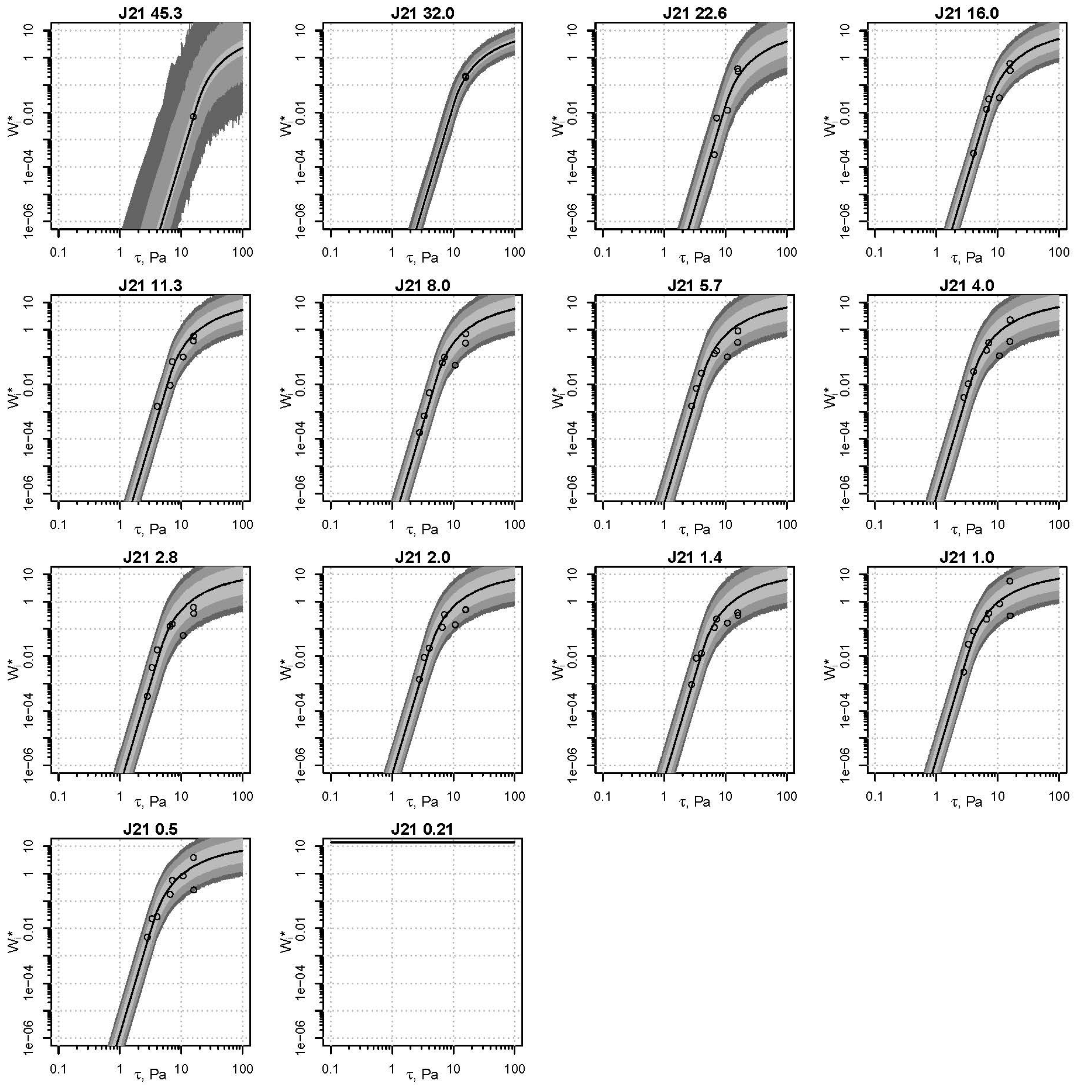
The overall positive monotonic theoretical relationship for sand content and transport, while not directly inferred from the analysis, is still likely given the variability of the parameters. Figure 10 shows an example the fractional rating curves for the J21 sediment. The results in this and related figures [25] indicate that the model is generally able to infer a reference stress distribution that produces predictions consistent with the observations. While the rating curves generally seem to be appropriate, there is one suspect rating curve, that for the 32.0 mm size fraction. This size fraction had only two closely spaced observations, such that the posterior distribution is surprisingly narrow compared to the 45.3 mm posterior of the same figure, which has only one observation. The variance for the 32.0 mm fraction is evidently not representative of the true process. This shortcoming is not unique to a Bayesian approach, but is a general limitation and constraint that accompany these data. To compensate for this, a more specific prior for the variance parameter could be specified.

Figure 9. Individual sediment comparisons of original reference stress curves from Wilcock and Crowe [6] to inferred curves from Bayesian Model. Error bars are those from Wilcock and Crowe [6]. Credible intervals are color coded from darkest to lightest for 95%, 90%, and 68%. The 0.707 mm value was jittered so as to not overplot for J06. The solid black line shows the standard Shields Curve for incipient motion of uni-size sediment.

Figure 9. Individual sediment comparisons of original reference stress curves from Wilcock and Crowe [6] to inferred curves from Bayesian Model. Error bars are those from Wilcock and Crowe [6]. Credible intervals are color coded from darkest to lightest for 95%, 90%, and 68%. The 0.707 mm value was jittered so as to not overplot for J06. The solid black line shows the standard Shields Curve for incipient motion of uni-size sediment.

Figure 10. Posterior predictive distribution for J21, color coded darkest to lightest for the 95%, 90%, and 68% credible intervals.

Figure 10. Posterior predictive distribution for J21, color coded darkest to lightest for the 95%, 90%, and 68% credible intervals.

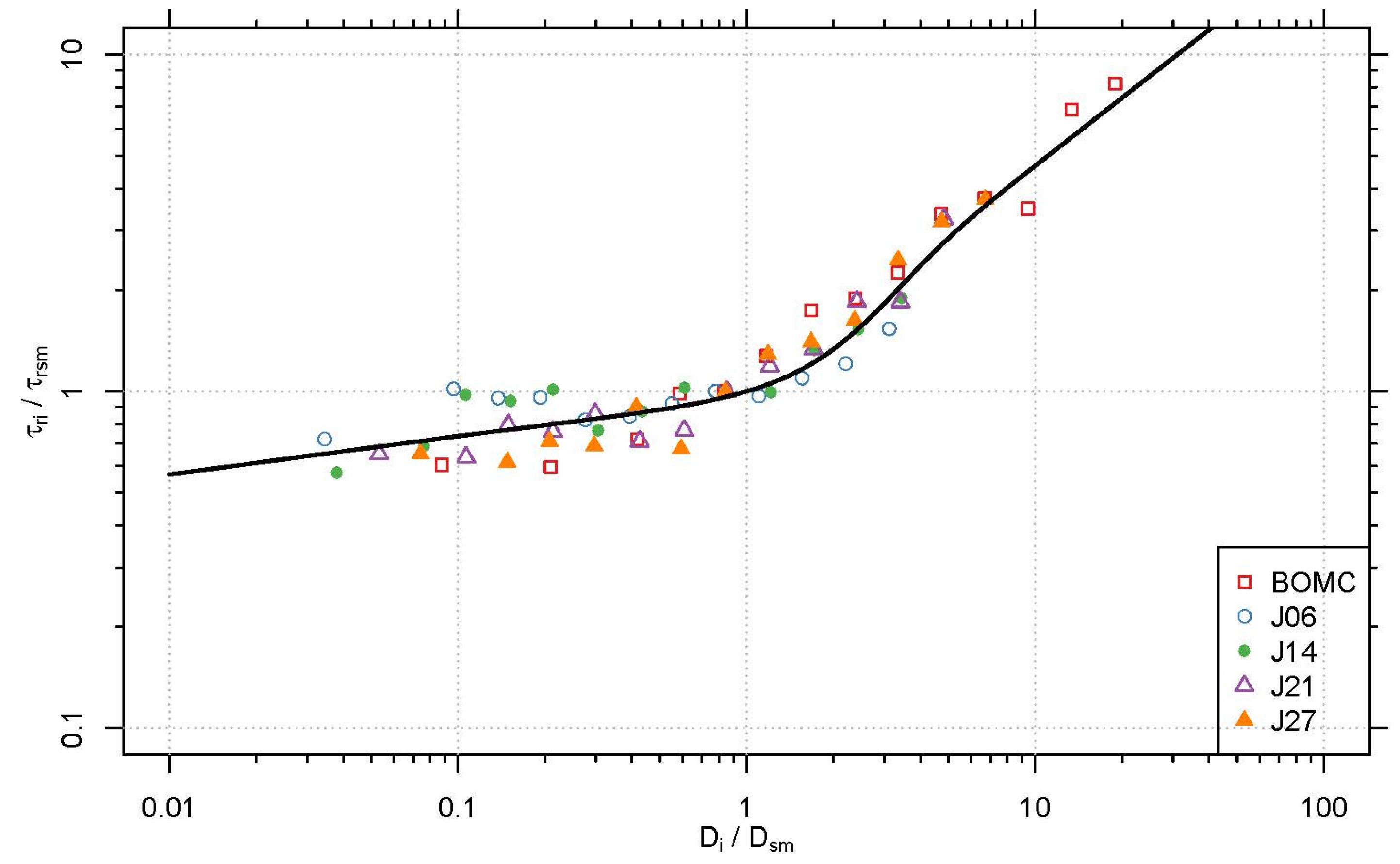
The inferred reference stresses in Table 2 can be used to construct a plot of the Wilcock-Crowe hiding function, which plots the ratio of the reference stress for a given size fraction to the reference stress of the surface geometric mean particle size against the ratio of the grain diameter of a given size fraction to the ratio of the geometric mean surface grain diameter. Thus, Figure 11 shows how the reference stress for a given size fraction can collapse into a single relation when scaled by the geometric mean particle size reference stress and diameter. This relationship was a central finding of Wilcock and Crowe ([6], Figure 4) and resulted from the manually calibrated reference stresses. In this research, the reference stresses were inferred from the Bayesian multi-fraction model and yield a similar trend.

Another central result from Wilcock and Crowe ([6], Figure 5) was the observation that the reference shear stress of the entire sediment mixture varies with sand content. It was observed that the reference stress of the geometric mean particle size of the mixture—the grain size used to scale the hiding function—decreased with increasing sand content and a model to describe this change in reference stress was proposed

$${\tau }_{rm}^{*}={\theta }_1+{\theta }_2\exp \left[-{\theta }_3{F}_s\right]$$

(13)

with the published result

$${\tau }_{rm}^{*}=0.021+0.015\exp \left[-20F_s\right]$$

(14)

Figure 11. Hiding function using inferred mean surface size reference stresses give valid results when compared to the manually-estimated parameter values used to construct the original similarity collapse of Figure 6 in Wilcock and Crowe [6].

Figure 11. Hiding function using inferred mean surface size reference stresses give valid results when compared to the manually-estimated parameter values used to construct the original similarity collapse of Figure 6 in Wilcock and Crowe [6].

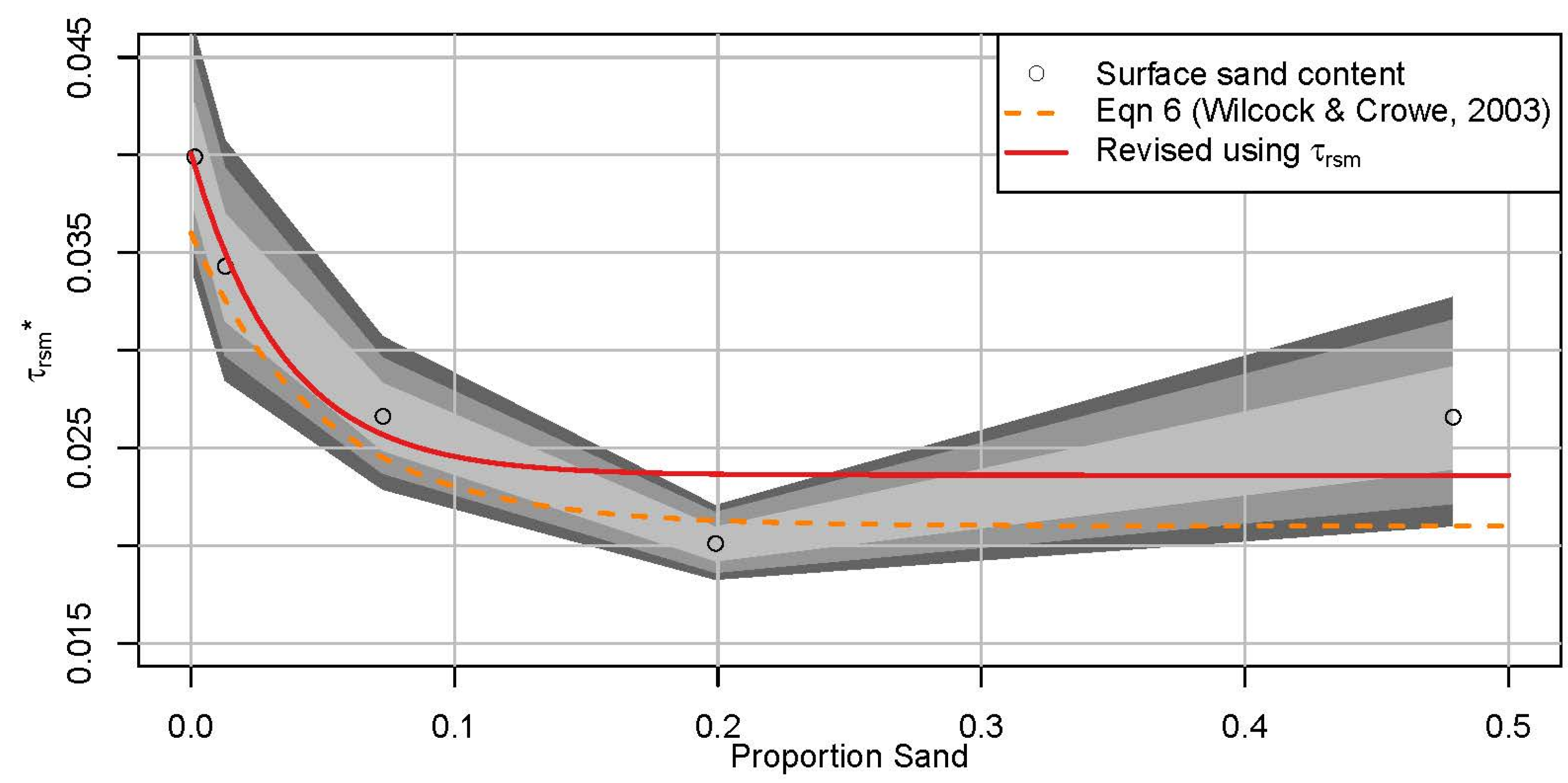
Figure 5 of [6] was updated using the inferred parameter values for reference stress and is included as Figure 12. The original formulation for describing the change in the reference stress of the mean particle size class is plotted as a dashed line in Figure 12. Because there is significant variability in the right-most point (corresponding to the inferred mean reference stress for BOMC), a new relationship was fitted to these data points using NLS:

$${\tau }_{rm}^{*}=0.024+0.016\exp \left[-28F_s\right]$$

(15)

Figure 12. Reference Shields stresses for the mean size of the bed surface ${\tau }_{r,sm}^{*}$ plotted against proportion sand on the bed surface, with credible intervals, color coded darkest to lightest for 95%, 90%, and 68%.

Figure 12. Reference Shields stresses for the mean size of the bed surface ${\tau }_{r,sm}^{*}$ plotted against proportion sand on the bed surface, with credible intervals, color coded darkest to lightest for 95%, 90%, and 68%.

While a new equation can be fitted to the plotted points, this does not change the fact that there the right-most point exerts leverage and requires the entire flat portion of Equation (15) and Figure 12 to be elevated. The posterior distribution of the geometric mean surface grain size reference stress was used to construct a credible interval, plotted in Figure 12. Here we see that the variation in the reference stress alone could account for significant spread in the resulting Equations (13) through (15).

Another central result from Wilcock and Crowe ([6], Figure 5) was the observation that the reference shear stress of the entire sediment mixture varies with sand content. It was observed that the reference stress of the geometric mean particle size of the mixture—the grain size used to scale the hiding function—decreased with increasing sand content and a model to describe this change in reference stress was proposed

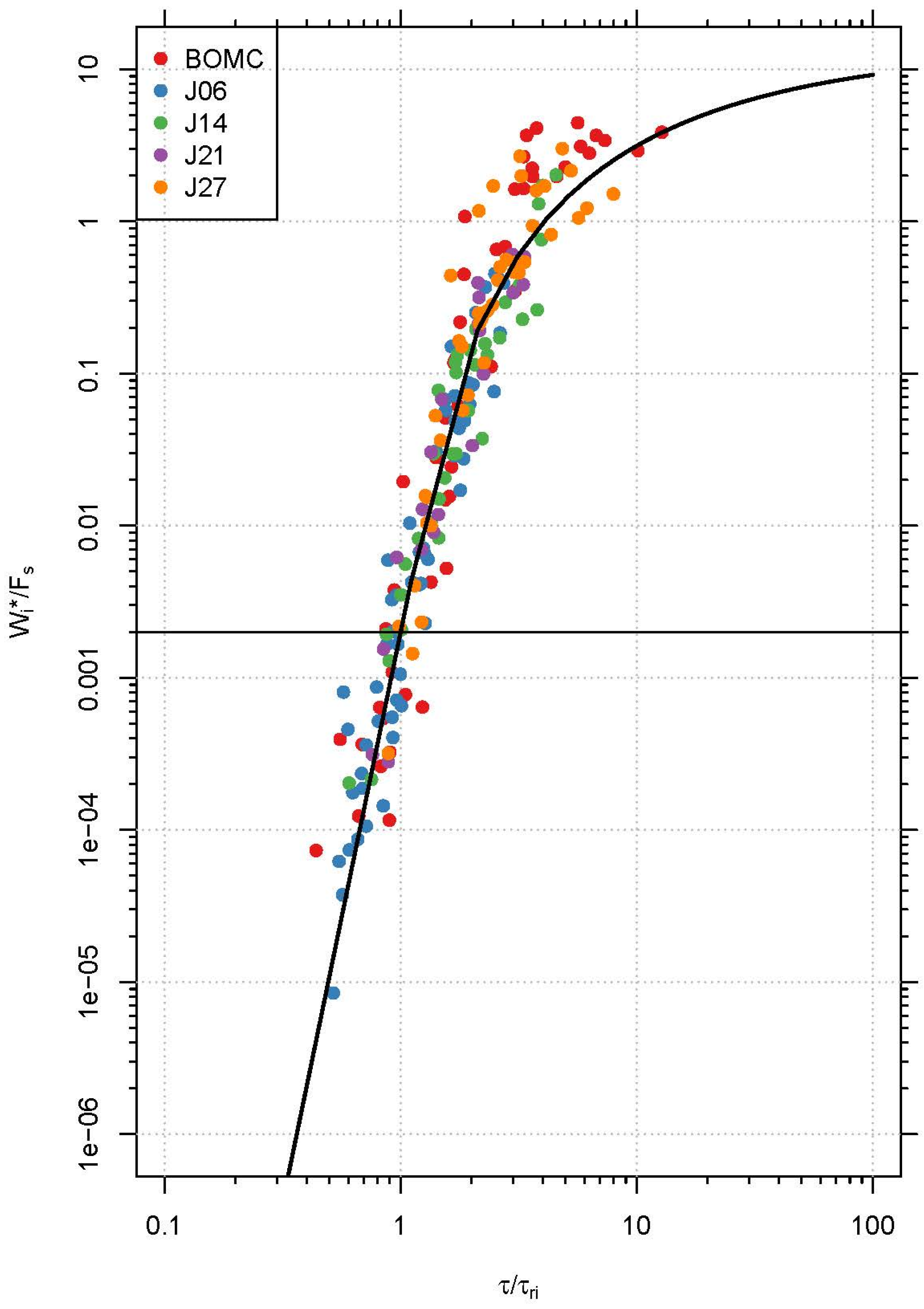
Figure 13 shows the fractional similarity collapse constructed using the inferred reference stresses for each grain size class and sediment mixture. This figure is comparable to Figure 6 of Wilcock and Crowe [6] and demonstrates that the estimated parameters from the Bayesian model are able to give valid results when compared to the manually-estimated parameter values used to construct the original similarity collapse of Figure 6 in Wilcock and Crowe [6].

Figure 13. Fractional similarity collapse for multifraction observations and model prediction. The bold line though the data is the calibrated multifraction Wilcock-Crowe Equations (2)–(6) for the multifraction transport data). W* = 0.002 is the reference value that corresponds to the reference shear stress τ_r.

Figure 13. Fractional similarity collapse for multifraction observations and model prediction. The bold line though the data is the calibrated multifraction Wilcock-Crowe Equations (2)–(6) for the multifraction transport data). W* = 0.002 is the reference value that corresponds to the reference shear stress τ_r.

3.2. Discussion

3.2.1. General

The Bayesian fractional transport model developed here has reasonable inferential and predictive power. The first indication of this success is in the positive indications from the numerical method diagnostic plots, the trace plots and posterior histograms. A second and more convincing indication of model validity is the general correlation of the manually/expert-fitted reference stress curves with those inferred from the model.

Several figures communicate this feature of the analysis, including Figure 8 and Figure 9. In Figure 9, there is no instance in which the error bars and credible interval infer a distinct region. The error bars set by Wilcock and Crowe [6] are generally conservative relative to the 95% credible interval. For example, J06, J14, and J27 have numerous points that assume wider error bars than the credible interval. Small diameters of J06 have almost twice the interval width. One possible explanation for this is that the Wilcock and Crowe [6] ranges were manually determined and represent values (no formal confidence interval associated with it) that provide a visual estimate of the broadest possible fit. Thus, all of the variability in the predictions was assumed to come from variation in the reference stress parameter. In the Bayesian model, there are two components that contribute to overall variation—reference stress and the variance parameter. Thus, the reference stress credible intervals of the Bayesian model represent true parameter variability, and the variance parameter represents the manual values are much smoother and are closer to monotonicity than the Bayesian estimates. As discussed briefly before, one would expect a positive monotonic relationship between sand and transport, so while the manual fitting is likely influenced by this overarching thought, the Bayesian estimates are independent of the monotonic assumption. However, the credible regions do show a consistent monotonic trend with only a few slight exceptions (e.g., J14).

The fractional posterior densities in Figure 7 show some hints of bi-modality in the reference stress parameter. There are also other posteriors that resemble a heavy-tailed, non-Gaussian distribution (see, for example, the posterior for the 45.3 mm size fraction of J21). As discussed in [12], traditional methods of parameter inference (e.g., NLS or weighted least squares) cannot be easily modified to accommodate this type of result. A feature of the inferred data is that the form of the parameter estimates is an outcome of the Bayesian methodology through a simple evaluation of the posterior distribution. Further, the original error bars in Figure 3 of Wilcock and Crowe [6] do not specify how the values are distributed between the limits. This information is provided by the Bayesian approach.

Figure 7 also illustrates the effect of sand content on mobility of individual fractions. For instance, the 0.5 mm panel shows that the mobility of sand fractions is highly dependent on bulk sand content, explaining why five distinct posterior distributions of reference stress have overlap only in their tails.

The success of the adaptive component of the MCMC algorithm is a significant model development. Because previous models were developed from only a few sediments and a single size fraction, manually tuning these models for numerical stability, despite being an iterative trial and error process, was a manageable modeling cost. To manually fit numerous sediments each with 13 size fractions would have made fitting the model impractical. Further, previous models only required the specification of one tuning variance, for the reference stress, because the prior distribution for the sediment transport variance parameter Equation (11) was an inverse gamma distribution, which is conjugate with the likelihood Equation (9) and therefore can be sampled via the Gibbs sampler for which a tuning variance is not required. Because the prior for σ was changed to a non-conjugate prior distribution, the MCMC algorithm then requires two tuning variances. To fit all the fractional models in this method requires tuning 130 parameters. An adaptive MCMC algorithm was needed to make such a process practical.

3.2.2. Hiding Function and Similarity Collapse

Using the calibrated model parameters from their analysis, Wilcock and Crowe [6] explored the relations between reference stresses, fraction grain size, and sand content. They developed a hiding function, Equations (3) and (4), similar to those previously developed by Ashida and Michue [15] and Parker et al., [3], to describe the shear stress needed to entrain different size fractions of a given mixture. Figure 11 shows the original hiding function as developed by Wilcock and Crowe [6] and the plotted points using the Bayesian estimates for τ_r,sm. The hiding function fitted to the inferred reference stresses does not suggest any deficiencies of the original function. By comparing Figure 3 of [6] to Figure 11 in the present analysis, the only discerning feature is that the Bayesian fit seems to have more uncertainty than the original fit as judged by the spread of the data points in the figure.

Prediction of the reference stress for the mean grain size of the bed surface τ_r,sm controls the overall mobility of the mixture. Wilcock and Crowe [6] plotted τ_r,sm versus sand content and demonstrated that the overall mixture mobility depends on the sand content of the bed (Equation (14), Figure 12). The notion that τ_r,sm would decrease with increasing sand content was a departure from previous thought. The fitted relation used the best estimate for the reference stresses and was sensitive to uncertainty in the data because only five points (one for each sediment mixture) were available to fit the trend. As established above, the reference stresses are distributions and are not fixed. The analysis leading to Equation(14) had no basis for accounting for uncertainty in the five values of τ_r,sm. Using the posterior mean values for the mean surface stresses, the present analysis resulted in a somewhat different relationship Equation (15), with the reference stress for BOMC being larger than what was originally specified in [6] for the same sediment. Because τ_r,sm for BOMC is a leverage point, small shifts in its value result in larger changes to the trend. The reference stress itself is a random variable, and if we account for this, credible intervals can be developed (Figure 12). The regions defined in Figure 12 generally support the validity of the original equation, especially when one considers that for each of the 9–10 flume experiments for a given sediment, the mean surface diameter, while well-defined, also had some variability.

To some extent, the validity of Equation (14) is a moot point under a Bayesian approach because this method of parameter estimation can infer the value of τ_r,sm directly. Although the original relation for τ_r,sm proposed by Wilcock and Crowe [6] (14) and the modified relation developed here Equation (15) are largely contained within the credible regions in Figure 12, the new relation Equation (15) exceeds the credible interval for a surface sand content of 20%. Thus, while prediction of τ_r,sm using the proposed equations is not needed for a Bayesian implementation of this sediment transport model, the original equation is supported by the Bayesian model results.

The final component of the multi-fraction model is the similarity collapse, shown as Figure 13. Each fractional transport observation is plotted using each size fraction’s posterior mean value divided into the observed skin friction shear stress, giving the x-axis ratio τ/τ_r,j. The results indicate that the model parameters estimated by the Bayesian algorithm provide a well-defined similarity collapse quite similar to that originally produced in Figure 6 of [6]. Any of the sensitivities that were observed in the hiding and Shields parameter variation plots are not an issue in the similarity collapse indicating that the general similarity phenomenon is a robust characteristic of sediment transport rather than an experiment-specific result. In the linear portion of the curve (τ/τ_r,j < 2) the data points are tightly and symmetrically clustered about the deterministic prediction, and the over-prediction that was observed in the bulk similarity collapse in Figure 3 does not appear to be an issue in the multi-fraction collapse. The original similarity collapse of Wilcock and Crowe [6] does not have this same symmetry in the linear region of the plot. However, the collapse shown in Figure 13 does suggest a small bias (under-prediction) relative to the observations, something that the original collapse in Wilcock and Crowe [6] does not have.

3.2.3. Motivation and Implementation on New Datasets

An underlying motivation for using a Bayesian approach is to provide a sound basis for quantifying uncertainty. The process of sediment transport is nonlinear and governed by factors that are more random variables than fixed values. Deterministic predictions of sediment transport, “on average”, do not explicitly account for the full range of interactions possible for a given set of conditions. The results of this paper demonstrate that the Bayesian approach provides valid estimates of model parameters for multi-fraction sediment transport and, therefore, a sound basis for assessing uncertainty. It is widely understood that randomness and variability are key components of the sediment transport process, so a model that makes it possible to leverage advances in multi-fraction transport prediction (such as the Wilcock-Crowe equations) with robust inference of the parameters and predictions as random variables (the Bayesian approach) provides an answer to problem of accounting for and managing uncertainty in sediment transport processes.

Kirchner et al. [25] observed that for a given sediment mixture, a multiplicity of bed configuration and transport rates are possible. This phenomenon, while understood and widely accepted, has no general solution. Sediment transport predictions may be calibrated to observations, but calibration results in point predictions for quantities better considered as random variables. This problem of fitting a transport relation is generally challenging enough in practice that formal assessment of uncertainty is generally not attempted. Without a formal method of quantifying the uncertainty, the only practical option is a manual perturbation analysis to assess the range of parameter values. Doing this type of analysis for 65 different sediment runs (13 sediment fractions for five different sediments) is time-consuming and prone to error. Further, as discussed in a previous section, doing this for one parameter (reference stress) is likely feasible, but including an additional parameter (e.g., variance) in a conventional analysis makes it impractical to sort out parametric and other variability.

In the present paper, the Wilcock-Crowe equation is calibrated to observations with the primary calibration parameter being reference stress. There are numerous ways of calculating the boundary stress of a river or flume, but what is largely unknown is how the total boundary stress is partitioned into skin friction. This partitioning is largely due to complex, changing bed configuration that is driven by the flow and transport itself. Using observed transport rates to calibrate the reference shear stress effectively accomplishes the partitioning of the total boundary stress into skin friction (or grain stress) and form drag (stress acting on the dunes, bars, and banks which does not contribute to grain movement) Wilcock (2001) [18]. The approach offered in this paper provides a robust means to determine reference stress and effectively address the drag partition problem.

In addition to estimation of parametric uncertainty, an ability to quantify risk associated with predictions is extremely valuable. There are a variety of situations in which the preferential transport of one size fraction relative to another is of interest. This may be to remove a certain range of sizes (e.g., flushing fines from a gravel bed for spawning habitat improvement), retain a certain fraction (e.g., contaminated sediment mobility), or simply assess mobility of a given size class (e.g., economically valuable grains). The bulk transport approach does not permit such questions to be answered. The model developed here allows for an estimation of risk on a size class basis. Where traditional methods provide a deterministic estimate of mobility, the approach described here provides a probability-based mobility assessment and makes it possible to achieve an estimate of the likelihood of mobilizing one grain size under conditions that would mobilize another. Traditional transport models cannot do this.

For application with a new transport dataset, the fractional transport data (of an arbitrary number of size fractions) can be evaluated using Equation (8). In this capacity, the general form of the sediment transport curve would be the Wilcock-Crowe equation, which would essentially be calibrated for the new dataset. Because the calibration (i.e., the Bayesian parameter estimation procedure) directly specifies the reference stresses for all of the particle size classes, the elements of the Wilcock and Crowe [6] model for specifying reference stress are not necessary (Equations (3)–(6) and (14)). This simplifies the overall approach and likely has the effect of reducing uncertainty because, as was shown previously, the variation of Shields stress with sand content was sensitive to the inferred reference stress of BOMC.

4. Conclusions

We present a multi-fraction Bayesian sediment transport model developed using the Wilcock-Crowe equations and sediment transport data from mixed-size sediment transport experiments [8]. The Bayesian model was fitted to these transport observations and the resulting posterior distributions were analyzed and compared to transport model developed by Wilcock and Crowe [6]. The bulk model posterior distributions were compared to NLS estimates of model parameters as a verification that the Bayesian code was working correctly and the derived relationships originally produced as the Wilcock-Crowe equations were evaluated using the Bayesian posterior distribution results. We found that the Bayesian model generally provides an accurate and useful tool to robustly estimate model parameters, though small differences in some detail of the Wilcock-Crowe equations (the hiding function and relation for incipient motion of the mixture) were observed for the sandier mixtures.

From a modeling perspective, a fractional transport approach increases the dimensionality of the model from two parameters (bulk reference stress and variance) to 2 × k size fractions dimensions. Also, the prior distribution for the variance parameter was changed from an inverse gamma distribution used in prior work with single fraction/aggregated transport [4] to a lognormal distribution to overcome some constraints identified in previous work. The model was developed using observations for five mixed-size sediments of 13 fractions each, resulting in an estimation of 130 parameters. This increase in dimensionality is significant as it presents a more complete description of sediment transport processes, but brings along with it an increased demand on the MCMC algorithm. While multiple Markov chains could be spawned (for example, one for each size fraction), each Markov chain must be run sequentially thereby disallowing parallel computations for a single fraction. Previous research manually tuned the MCMC algorithm by specifying the tuning variances for the reference stress parameter. Because previous Bayesian transport models did not consider numerous sediments and size fractions, manually tuning was an acceptable task. In the multi-fraction model, manually specifying 130 parameters in an iterative framework is impractical, so an adaptive algorithm was developed to mitigate the increase in number of dimensions. The AMCMC algorithm showed good convergence on both the model parameters as well as the numerical method tuning parameter to the degree that model diagnostic plots confirm convergence on the target posterior distributions.

Predictive distributions were developed for both the bulk and fractional transport rating curves and closely agree with the observations and the relations manually fitted by Wilcock and Crowe [6]. Some difference was observed for larger particle sizes, owing to the fact that these fractions were immobile for many runs, such that the data set had few observations of large particle movement. Future work should provide a way of managing the zero-transport events so that the information from the experiments in which there was no measurable transport.

The model we developed is suitable for use in multi-fraction sediment transport, and the next steps involve applying the methodology to transport events in gravel bedded rivers where the transport of multiple fractions is being measured. Possible applications of this concept include the development of a two-fraction (sand and gravel) model, application to suspended sediment transport, and development of model code that is distributable for wider use by practitioners. Particularly relevant to coastal sedimentation problems is the observation that as sediments are transported from the mountains, into the piedmont, onto the coastal plain, and then into the estuaries, the bed grain sizes and transported fractions are constantly adapting to slope, stress, and relative proportions, making multi-fraction transport particularly important to coastal geomorphology and sediment transport.

The Bayesian method developed here provides a sound basis for quantifying uncertainty in mixed-size sediment transport. Sediment transport arises from complex, nonlinear interactions among flow, bed grain size, and transport. Data scatter and uncertainty are persistent components of the process and a Bayesian approach provides the ability to robustly infer model parameters and predictions as random variables. The method presented here provides a means to account for and manage uncertainty in sediment transport applications.