Investigating the Joint Probability of High Coastal Sea Level and High Precipitation

Abstract

The design strategies for flood risk reduction in coastal towns must be informed by the likelihood of flooding resulting from both precipitation and coastal storm surge. This paper discusses various bivariate extreme value methods to investigate the joint probability of the exceedance of thresholds in both precipitation and sea level and estimate their dependence structure. We present the results of the dependence structure obtained using the observational record at Bridgeport, CT, a station with long data records representative of coastal Connecticut. Furthermore, we evaluate the dependence structure after removing the effects of harmonics in the sea level data. Through this comprehensive analysis, our study seeks to contribute to the understanding of the joint occurrence of sea level and precipitation extremes, providing insights that are crucial for effective coastal management.

1. Introduction

Climate change and sea level rise play a major role in the risk of flooding in coastal areas [1]. Coastal flooding and erosion can result from several factors such as storm surges, tsunamis, subsidence, and high rainfall events, as discussed in [2,3]. Rising mean air temperature and sea level will increase the expected frequency of these events [4], and this has prompted the need for the development of designs for interventions to reduce impacts. There is wide geographic variability in the relative importance of these flooding mechanisms. Many coastal communities are located in bays or separated from the ocean by islands and are, therefore, sheltered from the direct effects of long period and high amplitude ocean waves. However, wind-driven storm surges freely propagate into bays to cause coastal flooding. Many other towns have been established near the mouths of rivers where they are vulnerable to flooding caused by high precipitation or snow melt in the watershed. The construction of seawalls or levees is often considered as a flood defence measure to address all three of these threats. However, a significant disadvantage of the approach is that the management of storm water during high precipitation rates is made more difficult. Retention basins and pumps are often employed and the system design must be informed by the joint probability distribution of high rainfall rates and high water level/wave heights.

Extreme value analysis ([5]) is usually employed to develop design criteria for hazard mitigation projects. Univariate extreme value analysis has been extensively studied in offshore and coastal safety by investigating the behavior of coastal wave heights [6,7], wind speed [8], and precipitation [9,10]. Insurance companies are also interested in assessing the risk from weather extremes, in order to design strategies to cope with, and adapt to, increased risks and expected damages [11]. The most popular univariate extreme value methods include Peaks Over Threshold (POT) by the Generalized Pareto Distribution (GPD), as well as the Block Maxima approach [5]. While univariate extreme value methods are a useful tool to investigate extreme behavior of individual events, bivariate extreme value methods should be employed when the co-occurrence of extremes in two processes must be considered.

Modeling the joint behavior of two or more events provides valuable insights into the likelihood and severity of extreme events, leading to more effective risk management strategies. For instance, the authors of [12] discuss modeling wave extremes by capturing the dependence among storm intensity, directionality, and intra-time distribution, offering improved boundary conditions for wave and near-shore analyses. In particular, traditional models for bivariate extremes are based on limiting joint distributions for the extreme values in each margin of a bivariate sample. Bivariate extreme value theory has been well developed and includes analogous extensions of the POT and Block Maxima approaches [5]. In addition, copulas [13] are also used as a popular choice to model the bivariate extremes. Copulas have extensive applications in storm modeling [14,15,16], hydrology [17,18,19], and coastal engineering [20,21]. For example, the dependence between observed water levels and precipitation, including impacts of sampling methods and distribution fitting and the resulting flood values, is explored using copulas in [22]. The joint distribution of rainfall and storm surge based on the copula function is investigated in [23]. The effect of internal climate variability on copula-based compound event analysis is studied in a case study in the Netherlands by [24]. Ref. [25] provides a review of commonly used techniques for estimating the tail dependence of a joint distribution. Ref. [26] discusses a tail dependence matrix, where a multivariate dependence measure is constructed using this bivariate tail dependence structure.

In this paper, we employ various bivariate extreme value methods to estimate the dependence between sea level and precipitation based on their joint probability of exceedances. By modeling the joint behavior of two variables, we can evaluate the dependence between the two variables in their extremes. We discuss and summarize the results from various bivariate extreme value analysis methods with respect to the bivariate sea level and precipitation data from Bridgeport, CT. Our goal in this study is to (i) explore various bivariate extreme value methods to estimate the dependence structure on the bivariate data, and (ii) compare the dependence structure between sea level and precipitation in the presence and absence of tidal harmonics. Of course, at some sites, river flow and water level, or wave conditions, may have to be considered, so in the discussion section we comment on how the methods we have considered may be extended to more than two variables.

The format of this paper follows. Section 2 describes the bivariate daily maximum sea level and precipitation data from Bridgeport, CT. Section 3 discusses different bivariate extreme value methods for modeling the joint behavior of two variables and discusses the dependence structure. In Section 4, we discuss the dependence structure between sea level and precipitation after adjusting for sea level harmonics.

2. Data Description and Exploration

We analyze data with regard to two variables, sea level and precipitation, to investigate the dependence in their extremes. Observations on sea level have been recorded at hourly intervals from approximately 200 water level gauges across various locations in the United States by the National Oceanic and Atmospheric Administration (NOAA) and predecessor agencies. The data are shared through an interface at https://coastwatch.pfeg.noaa.gov/erddap/tabledap/ accessed on 17 May 2023. The hourly data are measured with respect to the North American Vertical Datum of 1988 (NAVD 88), which is the official vertical datum of the United States used as a reference system by surveyors, engineers, and mapping professionals to measure and relate elevations to the Earth’s surface [27] and is recorded in meters. Therefore, the sea level data has negative values, corresponding to the observations below the reference point.

Data on precipitation were obtained from the NOAA National Climatic Data Center, which archives 24 h precipitation totals for numerous stations in the United States recorded in inches. Ref. [28] describes the database known as the Global Historical Climatology Network (GHCN)-Daily dataset, which contains daily data from over 80,000 surface stations worldwide, about two-thirds of which are for precipitation alone.

We analyzed sea level and precipitation data from Bridgeport, CT for the years 1970–2015. The sea level data are from the Bridgeport harbor, while the 24 h precipitation totals are from the Sikorsky Memorial Airport in Bridgeport. The time series plot of the two variables are shown in Figure 1. In the precipitation data, no precipitation was reported on $66\%$ of the days. The missing values in the daily maximum sea level data and the precipitation are handled using linear interpolation using the R package (R version 4.3.2) imputeTS.

We consider exploratory investigations on the bivariate data using trend analysis in Section 2.1. Next, we examine the tail behavior of each variable independently by conducting univariate extreme value analysis in Section 2.2. Section 2.3 describes the empirical joint behavior of sea level and precipitation.

2.1. Exploring Temporal Trend and Correlations

Although Figure 1 does not seem to indicate the presence of time trend, in general one can use various methods for verifying the presence of time correlation in the data summarized in

Table 1. Temporal trend and correlation analysis for precipitation and daily maximum sea level from the Bridgeport data.

Variable	Metric	Value (Interpretation)
	Mann-Kendall’s $\tau$	0.004142 (No Trend)
	Sen’s Slope	0 (zero slope)
Precipitation	Hurst exponent	0.5805 (No Persistence)
	Mann-Kendall’s $\tau$	0.1187 (Slight Trend)
	Sen’s Slope	0.000009 (small non-negative slope)
Daily Max Water Level	Hurst exponent	0.7281 (Moderate Persistence)

. The Mann–Kendall test and Sen’s slope test for a monotonic trend make minimal assumptions. Both the methods include an asymptotic z-test, where the null hypothesis is that the data do not follow a monotonic trend. The Mann–Kendall test [29] is a non-parametric, rank-based approach that determines the presence of a monotonic trend in time series data by estimating Kendall’s $\tau$. The Sen’s Slope [30] provides a nonparametric alternative to ordinary least squares regression, calculating the median of all possible slopes between pairs of data points of a given time series. As expected for precipitation, both the Mann–Kendall test and Sen’s slope fails to reject the null hypothesis (with a p-value of 0.5 for both methods), indicating an absence of a monotonic trend in the precipitation data. For the daily maximum sea level data, the the Mann–Kendall test and Sen’s slope rejects the null hypothesis (with p-values < 0.05), indicating a presence of a monotonic trend. However, a Kendall’s $\tau$ of $0.1187$ and a Sen’s slope of 0.000009 indicate a presence of a slightly positive trend with a small non-negative slope. We also investigated the presence of a time trend by conducting linear regression analysis, with day, month, and year as predictors. The regression analysis on precipitation shows no effect of time trend with an adjusted R-squared of $0.00152$, while the regression analysis on daily maximum sea level shows a slight effect of a time trend with an adjusted R-squared of $0.1056$.

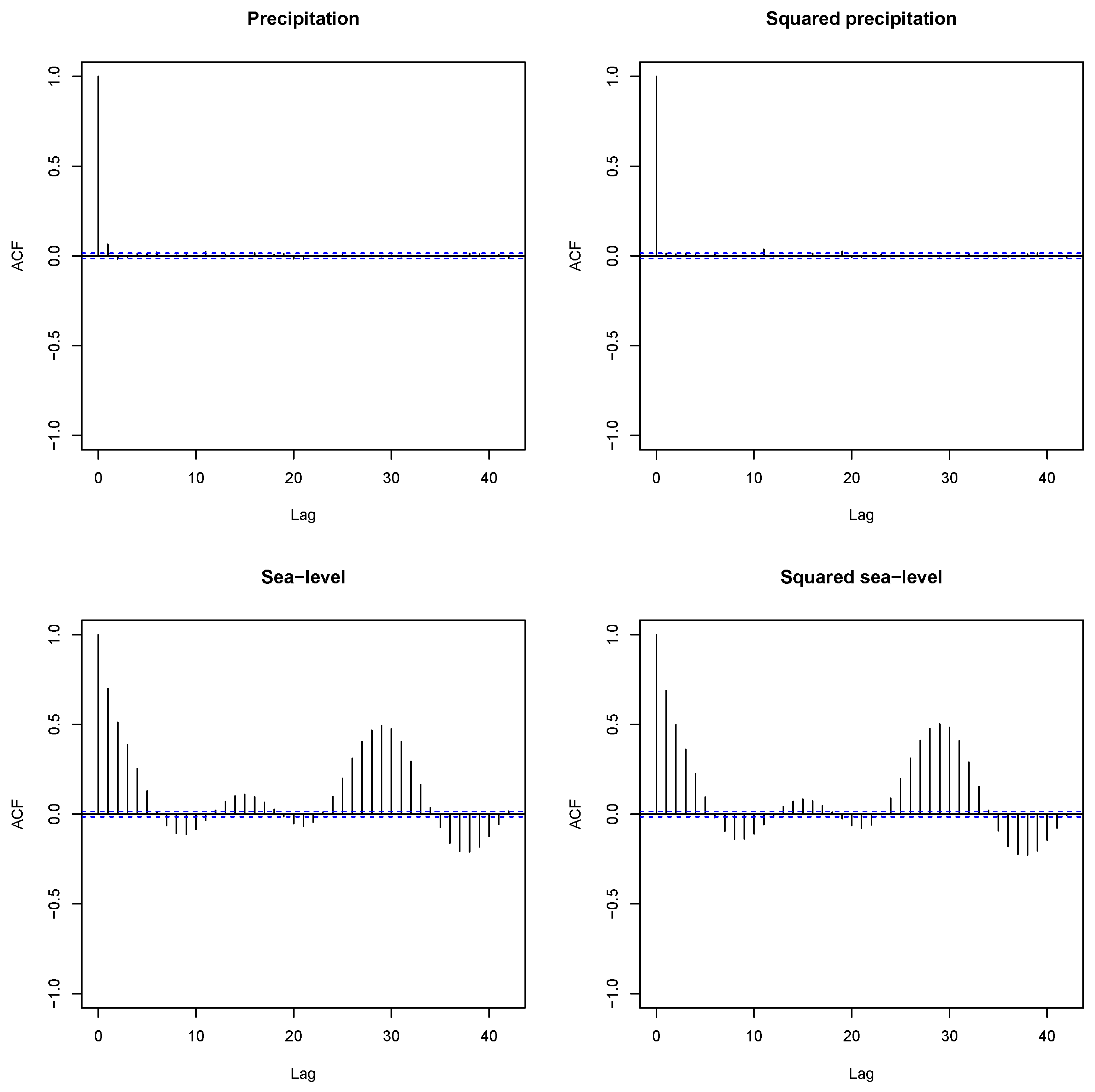
We investigated the temporal correlation in the data using the auto-correlation function (ACF). Figure 2 shows the ACF plots for precipitation, squared precipitation, daily-maximum sea level, and and squared daily-maximum sea level. The ACF precipitation and squared precipitation do not show any pattern indicating an absence of temporal correlation. The ACF of daily-maximum sea level and squared daily-maximum sea level show a presence of temporal correlation in the data. The Hurst exponent [31] is also estimated to measure long-range dependence in the time series, quantifying the series’ tendency to persist in a certain direction. The Hurst exponent H lies between 0 and 1, where $0<H<0.5$ indicates anti-persistent behavior, $H=0.5$ corresponds to random walk, and $0.5<H<1$ corresponds to persistent behavior). The value of the empirical Hurst exponent of 0.5805 indicates no persistent behavior in the precipitation data, while an empirical Hurst exponent of 0.7281 indicates the presence of moderate persistence in the daily maximum sea level data.

2.2. Univariate Extreme Value Analysis of Sea Level and Precipitation

We investigated the univariate extreme behavior by analyzing the daily maximum sea level and precipitation from 1970–2015 using the peaks over threshold (POT) by generalized Pareto distribution (GPD) approach [5,32]. The POT approach models observations that exceed a certain high threshold, say w. This consists of fitting a generalized Pareto (GP) distribution to the tail of the data that exceed a threshold w with a cumulative distribution function (c.d.f).

$$\begin{array}{c}\hfill F_w\left(y\right)=\left\{\begin{array}{cc}1-\left(1+\xi {\displaystyle \frac{y}{{\sigma }_w}}\right),\hfill & \xi \ne 0\hfill \\ 1-exp\left(-{\displaystyle \frac{y}{{\sigma }_w}}\right),\hfill & \xi =0,\hfill \end{array}\right.\end{array}$$

(1)

where $y>0$, ${\sigma }_w>0$, and $\xi \in \mathbb{R}$ (the real line). We implemented the POT method using the extrememix [33] R package, which employs a Bayesian framework to model each univariate data in order to estimate the GPD model parameters and threshold w. The maximum likelihood estimates of the GPD scale (${\widehat{\sigma }}_w$), shape ($\widehat{\xi }$), and threshold ($\widehat{w}$) for the sea level and precipitation data are shown in

Table 2. POT model estimates along with the standard errors based on the univariate extreme value analysis of daily maximum sea level and precipitation.

Variable	${\widehat{\mathit{\sigma }}}_{\mathit{w}}$	$\widehat{\mathit{\xi }}$	$\widehat{\mathit{w}}$
Sea level	$0.10$	$0.15$	$1.44$
Precipitation	$0.36$	$0.22$	$0.11$

.

Given the estimated GPD parameters, the return value, which is the value exceeded on average once every m years (return period), is computed as

$$z_m=\left\{\begin{array}{cc}w+{\displaystyle \frac{{\widehat{\sigma }}_w}{\widehat{\xi }}}[{\left(m{\widehat{\lambda }}_w\right)}^{\widehat{\xi }}-1],\hfill & \widehat{\xi }\ne 0\hfill \\ w+{\widehat{\sigma }}_{w}log\left(m{\widehat{\lambda }}_w\right),\hfill & \widehat{\xi }=0.\hfill \end{array}\right.$$

where ${\widehat{\lambda }}_w=P(Y>w)$. Figure 3 shows the return level plots for the sea level and precipitation data, with return values $z_m$ plotted across different values of return period m.

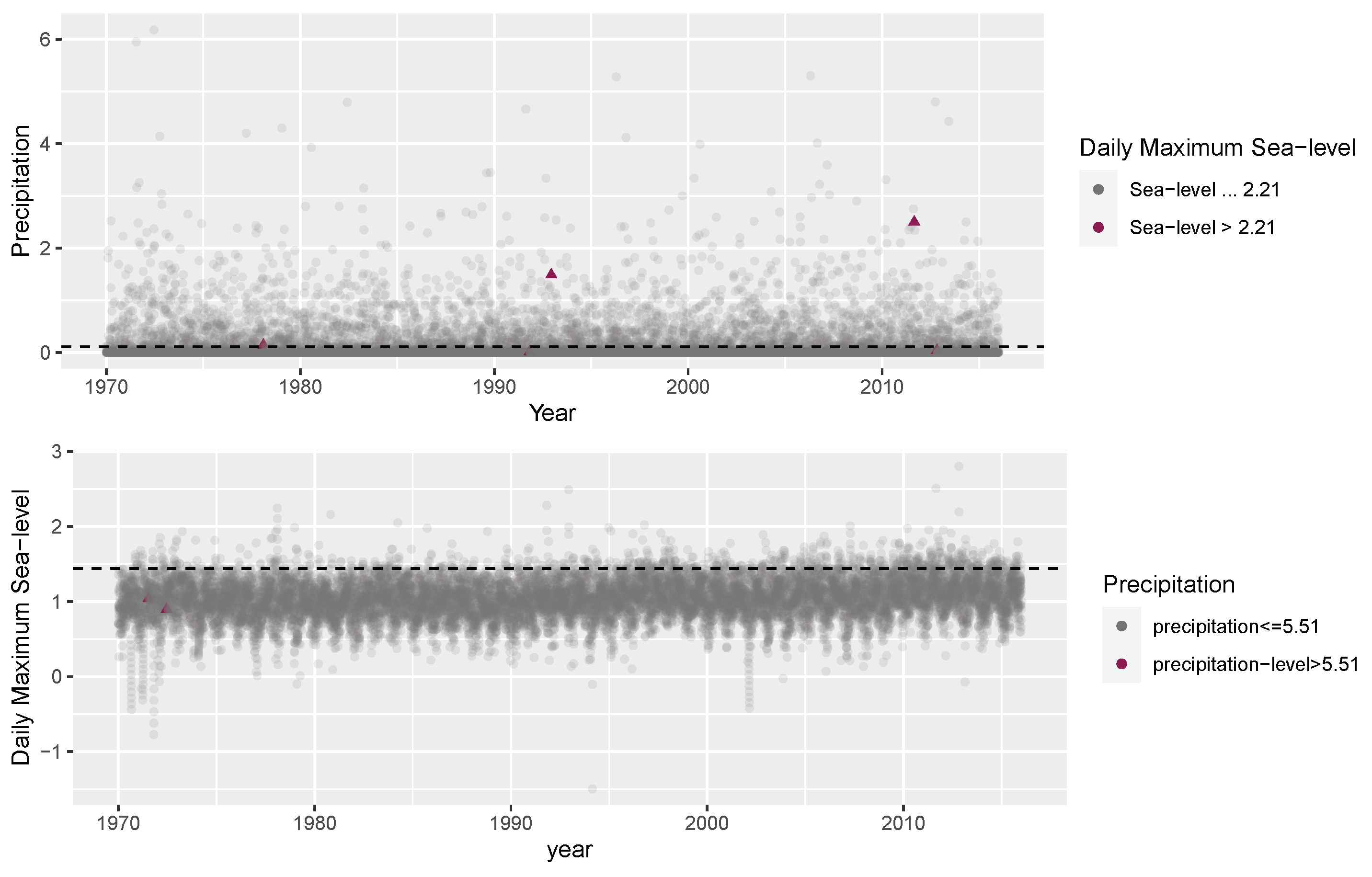
The return values for $m=10,50,100$ on daily maximum sea level and precipitation are shown in

Table 3. m-year return value estimates.

m-Year Return Value	Daily Maximum Sea Level	Precipitation
$m=10$	$2.21$	$5.51$
$m=50$	$2.60$	$8.54$
$m=100$	$2.79$	$10.22$

. We can leverage the m-year return value estimates of the daily maximum sea level (presented in Table 3) to examine precipitation behavior at time points where daily maximum sea level exceeds $z_m$. For instance, the first plot in Figure 4 shows the distribution of precipitation on days when the daily maximum sea level exceeds the 25-year return value. Similarly, the second plot in Figure 4 shows the distribution of daily maximum sea level on days when precipitation exceeds $z_m$. In Figure 4, we see that the days when the daily maximum sea level (or precipitation) exceeds the 10-year return value does correspond to higher values in the precipitation (or daily maximum sea level) data. Following the univariate exploration, we examine the empirical joint behavior of the two variables, described in Section 2.3.

2.3. Empirical Joint Behavior of Sea Level and Precipitation

It is important to study the joint behavior of daily maximum sea level and precipitations and investigate their dependence in order to characterize the likelihood of flooding resulting from both precipitation and coastal storm surge. This information can help design strategies for flood risk reduction due to sea level fluctuations and precipitation rates. We investigated the empirical joint dependence between the sea level and precipitation using Spearman’s rank correlation coefficient, a scatter plot, and a cross-correlation (CCF) plot. Spearman’s rank correlation coefficient [34] is a non-parametric measure of rank correlation that assesses the statistical dependence between the rankings of two variables and the degree to which the relationship between two variables is monotonic. Spearman’s rank correlation coefficient is estimated to be 0.1981 between precipitation and water level, indicating a weak positive monotonic relationship. The scatter plot shown in Figure 5 between the two variables does not show any linear trend. The cross-correlation plot shown in Figure 6 indicates the strength of the linear relationship between daily maximum sea level and precipitation at different lags. Figure 6 shows that the two variables have a maximum correlation at lag 0 with a correlation value of $0.18$. Thus, based on the empirical plots, the overall linear association between the two variables is weak.

In addition to the overall association, it is important to examine the co-occurrence of high precipitation at times of anomalously high water level in order to determine if the coastal project design needs to account for the potential consequences of extremely unlikely events due to the joint occurrence of high rainfall and high sea level. Figure 7 shows the empirical joint probability distribution function denoted by $P(X>x,Y>y)$ for the daily maximum sea level and precipitation data. The joint probability of high values of precipitation and rainfall is close to zero.

The dependence structure between two variables in the tail region can be evaluated using bivariate extreme value methods. A brief overview of various bivariate extreme value methods in the literature and the dependence measure obtained on the bivariate sea level and precipitation data based on each of the methods is described in Section 3.

3. Bivariate Extreme Value Analysis of Sea Level and Precipitation

In this section, we discuss different methods for modeling the joint behavior of two variables, including the bivariate threshold excess model, the copula-based approach, the maxima approach, and the L-comoments approach. A tutorial providing a practical guide on how to implement various bivariate extreme value approaches using R can be accessed from https://github.com/NamithaVionaPais/ accessed on 1 February 2024. Following this tutorial, a user can gain a deeper understanding of bivariate extreme value analysis and apply these methods to data of interest.

3.1. Bivariate Threshold Excess Model

Similar to the univariate POT by GPD approach discussed in Section 2.2, the goal of the bivariate threshold excess model is to estimate the joint distribution in the tail region. In the univariate case, the tail of the marginal distribution functions $F_X\left(x\right)$ and $F_Y\left(y\right)$ is approximated by a GPD distribution for suitable thresholds $w_x$ and $w_y$ with parameters $({\sigma }_{w_x},{\xi }_x)$ and $({\sigma }_{w_y},{\xi }_y)$, respectively. In the bivariate framework [5,35], the transformations

$$\tilde{X}=-(log\left\{1-{\xi }_x{\left[1+{\displaystyle \frac{{\xi }_x(X-w_x)}{{\sigma }_{w_x}}}\right]}^{-1/{\xi }_x}\right\}{)}^{-1}$$

and

$$\tilde{Y}=-(log\left\{1-{\xi }_y{\left[1+{\displaystyle \frac{{\xi }_y(Y-w_y)}{{\sigma }_{w_y}}}\right]}^{-1/{\xi }_y}\right\}{)}^{-1}$$

lead to variables $(\tilde{X},\tilde{Y})$ whose distribution function $\tilde{F}(x,y)$ has margins that are an approximately standard Fréchet distribution for $X>u_x$ and $Y>u_y$. Then, the joint distribution $\tilde{F}(x,y)$ is approximated as

$$\tilde{F}(x,y)\to G(x,y)=exp\{-V(x,y)\},$$

(2)

for $x>w_x,y>w_y$, where

$$V(x,y)=2{\int }_0^{1}max\left({\displaystyle \frac{\omega }{x}},{\displaystyle \frac{1-\omega }{y}}\right)dH\left(\omega \right),$$

(3)

and H is a distribution function on $[0,1]$ satisfying the mean constraint

$$\begin{array}{c}\hfill {\int }_0^1\omega dH\left(\omega \right)=1/2.\end{array}$$

(4)

There are a few choices of parametric families for H on $[0,1]$ whose mean is equal to $0.5$ for every value of the parameter. These include the logistic, bi-logistic, negative logistic, and Husler–Reiss families. The most popular choice is the logistic family defined by

$$\begin{array}{c}\hfill h\left(\omega \right)={\displaystyle \frac{1}{2}}({\alpha }^{-1}-1){\left\{\omega (1-\omega )\right\}}^{-1-1/\alpha }{\{{\omega }^{-1/\alpha }+{(1-\omega )}^{-1/\alpha }\}}^{\alpha -2},\end{array}$$

(5)

for $0<\omega <1$. The logistic family is popular due to the interpretation of the dependence between the variables using the parameter $\alpha$, where $\alpha \to 1$ corresponding to independent variables and $\alpha \to 0$ corresponding to perfectly dependent variables.

Given the choice of the parametric family H, the likelihood function (censored) is given by

$$\begin{array}{c}\hfill L(\theta \mid (x_1,y_1),\dots (x_n,y_n))=\prod _{i=1}^n\Psi (\theta \mid (x_i,y_i)),\end{array}$$

(6)

where

$$\Psi (\theta \mid (x,y))=\left\{\begin{array}{ccc}\frac{{\delta }^{2}F}{\delta x\delta y}{|}_{(x,y)},\hfill & \hfill & (x,y)\in [u_x,\infty )\times [u_y,\infty )\hfill \\ \frac{\delta F}{\delta x}{|}_{(x,u_y)},\hfill & \hfill & (x,y)\in [u_x,\infty )\times (-\infty ,u_y)\hfill \\ \frac{\delta F}{\delta y}{|}_{(u_x,y)},\hfill & \hfill & (x,y)\in (-\infty ,u_x)\times [u_y,\infty )\hfill \\ F(u_x,u_y),\hfill & \hfill & (x,y)\in (-\infty ,u_x)\times (-\infty ,u_y)\hfill \end{array}\right.$$

(7)

The censored likelihood treats the marginal observations below their thresholds as being censored at those thresholds. In R, there are several packages that can be used to conduct the bivariate threshold excess model, including evd, evir, POT, and extRemes. In the bivariate threshold excess model, we need to select appropriate thresholds $w_x$ and $w_y$ to evaluate the joint behavior in the tail region.

One method of selecting the threshold $u^{*}$ is to consider a function $r\left(z\right)$, where $r\left(z\right)=x_1\left(z_1\right)+x_2\left(z_2\right)$ and $x_j\left(z_j\right)={\displaystyle \frac{-1}{log{F}_j\left(z_j\right)}}$ for $j=1,2$, and $F_j$ is estimated empirically [36]. Then we can use a spectral measure plot, where integers $k=1,2,\dots n-1$ are plotted against $(k/n)r_{(n-k)}$. The largest value of k, denoted as $k_0$, for which $(k/n)r_{(n-k)}$ is close to 2, determines the pair of threshold values to be used. The R package evd provides the function bvtcplot for creating a bivariate threshold selection plot. Another way to select the threshold is to consider marginal distributions of POT modeled by a GPD approach that generates thresholds independently for each variable. Alternate threshold selection methods include the graphical diagnostic method [37], the probabilistic-based method [38], and the mixture method [39].

We fit the bivariate threshold excess model using the evd package to the precipitation and daily maximum sea level data by assuming a logistic family on H and a threshold selected using the bivariate threshold choice plot. The threshold estimated using this method is $0.19$ for precipitation and $1.29$ for the daily maximum sea level. The dependence parameter estimated is shown in the first row of

Table 4. Dependence parameter obtained from POT, the maxima approach, the copula method, and L-comoments.

Method	Dependence Parameter
POT	$0.8910$
Maxima approach	$0.7500$
L-comoments ${\tau }_2^{\left[12\right]}$	$0.3161$
L-comoments ${\tau }_2^{\left[21\right]}$	$0.2628$
Gaussian copula (Kendall’s $\tau$ )	$0.1738$

. The dependence parameter $\alpha$ from the POT approach being closer to 1 indicates a weak dependence between the daily maximum sea level and precipitation in the tail region. In particular, the value $\alpha \to 1$ indicates perfectly independent variables and $\alpha \to 0$ corresponds to perfectly dependent variables. In addition to the dependence parameter, we can also obtain the return value curves for probability levels $p=0.9,0.95,0.99$ shown in Figure 8a.

3.2. Maxima Approach

The maxima approach in bivariate extreme value analysis models the joint distribution of two random variables by focusing on their maxima over a defined block. We define ${\mathit{M}}_n^{*}=(M_{\tilde{x},n}^{*},M_{\tilde{y},n}^{*})=\left({\displaystyle \underset{i=1,2,\dots ,n}{max}}\left\{X_i\right\}/n,{\displaystyle \underset{i=1,2,\dots ,n}{max}}\left\{Y_i\right\}/n\right)$ as the scaled vector of componentwise maxima over a block size n. The goal of the maxima approach is to estimate the distribution of ${\mathit{M}}_n^{*}$ as $n\to \infty$. Following the standard univariate results of the block maxima approach, the marginal distribution of $M_{\tilde{x},n}^{*}$ and $M_{\tilde{y},n}^{*}$ is standard Fréchet. Then, following Theorem 8.1 in [5], the joint distribution function $P\{M_{\tilde{x},n}^{*}\le x,M_{\tilde{y},n}^{*}\le y\}$ is approximated as

$$\begin{array}{c}\hfill P\{M_{\tilde{x},n}^{*}\le x,M_{\tilde{y},n}^{*}\le y\}\stackrel{d}{\to }G(x,y),\end{array}$$

(8)

where G is a non-degenerate distribution function and has the form

$$\begin{array}{c}\hfill G(x,y)=exp\{-V(x,y\left)\right\},x>0,y>0\end{array}$$

(9)

where

$$V(x,y)=2{\int }_0^{1}max\left({\displaystyle \frac{\omega }{x}},{\displaystyle \frac{1-\omega }{y}}\right)dH\left(\omega \right),$$

(10)

and H is a distribution function on $[0,1]$ satisfying the mean constraint

$$\begin{array}{c}\hfill {\int }_0^1\omega dH\left(\omega \right)=1/2\end{array}$$

(11)

We fit the maxima approach using the evd package where the maximum is taken over six days, and we considered a (symmetric) logistic extreme value distribution to estimate the parameters of the joint distribution. The duration that a single storm system dominates the weather in the study area ranges between three and five days; consequently, a block size of six days ensures that all the extreme events are caused by independent events. The dependence parameter $\alpha$ from the maxima approach shown in the second row of Table 4 is closer to 1, indicating a weak dependence between the daily maximum sea level and precipitation over the block maxima of six days. In addition to the dependence parameter, we can obtain the return value curves for probability levels $p=0.9,0.95,0.99$ shown in Figure 8b.

3.3. L-Comoments—Multivariate Extensions of L-Moments

Multivariate L-moments, also known as L-comoments, extend the concept of L-moments to multivariate distributions. The L-comoment ratios [40] provide insights into the multivariate relationships, dependencies, and higher-order moments between the different components of the observed data. In the univariate setup, the $r^{th}$ population L-moment is defined as

$$\begin{array}{c}\hfill {\lambda }_r=r^{-1}\sum _{k=0}^{r-1}{(-1)}^k\left(\genfrac{}{}{0pt}{}{r-1}{k}\right)E\left(X_{r-k:r}\right),\end{array}$$

(12)

where $X_{k:n}$ represents the $k^{th}$ order statistic in a sample of size n.

Similarly in the bivariate setup, the $r^{th}$ population L-comoment of $X^{\left[1\right]}$ wrt $X^{\left[2\right]}$ is defined as

$$\begin{array}{c}\hfill {\lambda }_r^{\left[12\right]}=r^{-1}\sum _{k=0}^{r-1}{(-1)}^k\left(\genfrac{}{}{0pt}{}{r-1}{k}\right)E\left(X_{r-k:r}^{\left[12\right]}\right),\end{array}$$

(13)

where $X_{r-k:r}^{\left[12\right]}$ indicates the element of $\{X_1^{\left(1\right)},X_2^{\left(1\right)},\dots ,X_n^{\left(1\right)}\}$ that is paired with $X_{r:n}^{\left(2\right)}$ and $E\left(X_{r-k:r}^{\left[12\right]}\right)=nE(X_1^{\left(1\right)}\mid X_1^{\left(2\right)}=X_{r:n}^{\left(2\right)})$. An unbiased sample estimator for ${\lambda }_r^{\left[12\right]}$ [41] is given by

$$\begin{array}{c}\hfill {\widehat{\lambda }}_r^{\left[12\right]}={\displaystyle \frac{1}{n}}\sum _{j=1}^n{w}_{j:n}^{\left(r\right)}{x}_{j:n}^{\left[12\right]},\end{array}$$

(14)

where $x_{j:n}^{\left[12\right]}$ is the ordered sample, and the weights $w_{j:n}^{\left(r\right)}$ are computed as

$$\begin{array}{c}\hfill w_{j:n}^{\left(r\right)}=\sum _{i=1}^{minj-1,r-1}{(-1)}^{r-1-i}\left(\genfrac{}{}{0pt}{}{r-1}{i}\right)\left(\genfrac{}{}{0pt}{}{r-1+i}{i}\right)\left(\genfrac{}{}{0pt}{}{j-1}{i}\right)/\left(\genfrac{}{}{0pt}{}{n-1}{i}\right).\end{array}$$

(15)

Similar to ${\lambda }_r^{\left[12\right]}$, one can define the estimator for the $r^{th}$ L-comoment of $X^{\left[2\right]}$ with respect to $X^{\left[1\right]}$ denoted as ${\lambda }_r^{\left[21\right]}$. It should be noted that ${\lambda }_r^{\left[12\right]}$ and ${\lambda }_r^{\left[21\right]}$ are not necessarily symmetric. The L-comoment ratios defined as ${\tau }_r^{\left[12\right]}=\frac{{\lambda }_r^{\left[12\right]}}{{\lambda }_2^{\left[1\right]}}$ or ${\tau }_r^{\left[21\right]}=\frac{{\lambda }_r^{\left[21\right]}}{{\lambda }_2^{\left[2\right]}}$ for $r\ge 2$ are analogous to the univariate L-moment ratios, ${\tau }_r$. Specifically, when $r=2$, ${\tau }_2^{\left[12\right]}$ represents the L-correlation of $X^{\left[1\right]}$ with respect to $X^{\left[2\right]}$.

The lmomco package in R can be used to estimate the dependence measure, i.e., L-correlations ${\tau }_2^{\left[12\right]}$ and ${\tau }_2^{\left[21\right]}$. The L-comoments is fit to the bivariate precipitation and sea level data to estimate the dependence measure, i.e., L-correlations ${\tau }_r^{\left[12\right]}$ and ${\tau }_r^{\left[21\right]}$ shown in Row 3 and 4 of Table 4. These values indicate a weak association between the two variables.

3.4. Copula Approach

Copulas are a powerful tool for modeling the dependence between two or more variables. A bivariate copula is a function that links together univariate distribution functions of the two variables to model the joint bivariate distribution function. Sklar’s Theorem in [42] provides the mapping from the individual distribution functions $F\left(x\right),F\left(y\right)$ to the joint distribution function $F(x,y)$ as

$$F(x,y)=\mathit{C}\left(F\right(x),F(y\left)\right),$$

where $\mathit{C}$ is the copula function.

Table 5. Table describing different family of copulas and their association to Kendall’s $\tau$.

Copula	${\mathit{C}}_{\mathit{\alpha }}(\mathit{u},\mathit{v})$	Relation to Kendall’s $\mathit{\tau }$
Gumbel Copula	$exp\{-{[{(-lnu)}^{\alpha }+{(-lnv)}^{\alpha }]}^{{\displaystyle \frac{1}{\alpha }}}\}$	$1-{\displaystyle \frac{1}{\alpha }}$
Gaussian Copula	${\mathsf{\Phi }}_{\alpha }({\mathsf{\Phi }}^{-1}\left(u\right),{\mathsf{\Phi }}^{-1}\left(v\right))$	${\displaystyle \frac{2}{\pi }}arcsin\left(\alpha \right)$
Student t Copula	$t_{\alpha }(t^{-1}\left(u_1\right),t^{-1}\left(u_2\right))$	${\displaystyle \frac{2}{\pi }}arcsin\left(\alpha \right)$
Frank Copula	${\displaystyle \frac{1}{\alpha }}ln(1+{\displaystyle \frac{(e^{\alpha u}-1)(e^{\alpha v}-1)}{e^{\alpha }-1}})$	$1-{\displaystyle \frac{4}{\alpha }}\{D_1(-\alpha )-1\}$
Clayton Copula	$(u^{-\alpha }+v^{-\alpha }-1{)}^{-1/\alpha }$	${\displaystyle \frac{\alpha }{\alpha +2}}$

describes the different copulas and provides the relation between Kendall’s $\tau$ and the parameter values associated with the copula [43].

We fit the bivariate copula using the copula package in R to the bivariate daily maximum sea level and precipitation data. We fit various copulas using maximum likelihood estimation, and we chose the Gaussian copula as a suitable copula using the BIC criterion. The Kendall’s $\tau$ measure obtained from the Gaussian copula is shown in Row 5 of Table 4 and indicates a weak linear association between daily maximum sea level and precipitation.

Overall, the dependence measure obtained from various bivariate methods indicate a weak relationship in the bivariate daily maximum sea level and precipitation data. However, it is important to further examine the dependency after removing the periodic variations in the sea level data. Figure 9 shows a smoothed periodogram and auto-correlation function (ACF) plot of the hourly sea level data. These plots detect the presence of distinct periods, with the most prominent being $12.42065$, as shown in the periodogram. Therefore, it is crucial to further investigate the dependence once the influence of harmonics from hourly sea level data is removed. The results from the bivariate precipitation and daily maximum sea level after removing the effect of harmonics are presented in Section 4.

4. Dependence between Sea Level and Precipitation after Adjusting for Sea Level Harmonics

Tidal oscillations in ocean water level arise from the gravitational attraction between the earth, moon, and sun, and the centrifugal acceleration due to the rotation of earth around the center of mass of the earth–moon–sun system. The periods of the earth’s rotation and orbit around the sun, as well as the moon’s orbit, are reflected in the oscillations of the sea surface. Other more subtle effects, like the the oscillation of the axis of rotation of the earth, and the ellipticity of the orbits of the earth and moon add to the number of tidal frequencies, or tidal harmonics [44,45,46]. In shallow coastal areas, tidal oscillations are further complicated by nonlinear dynamic interactions that generate additional harmonic and sub-harmonic frequencies. More than a hundred harmonics can be detected, though most have a very small amplitude. The amplitude and phase of each frequency varies spatially, largely due to local bathymetric and coastal geometry effects, but once estimated from observations, accurate predictions can be made. By identifying and removing the effect of tidal harmonics in water level observations, one can further examine the dependence structure between the storm-forced sea level variations and precipitation.

To obtain the daily maximum sea level after removing the effect of harmonics, we investigated the behavior of the hourly sea level data to check for the presence of harmonics. We conducted a harmonic analysis on the hourly sea level data using the UTide Matlab (ver. R2021b) toolbox [47]. The unified tidal analysis can handle record times that are irregularly distributed and suitable for multi-year analyses. Once the harmonic analysis is conducted, we considered the daily maximum over the residuals from the harmonic analysis along with the precipitation as the input data for the bivariate extreme value analysis. The results from the bivariate precipitation and daily maximum sea level after removing the effect of harmonics is presented in

Table 6. Dependence parameter obtained from POT, the maxima approach, the copula method, and L-comoments.

Method	Dependence Parameter
POT	$0.7984$
Maxima approach	$0.7234$
L-comoments ${\tau }_2^{\left[12\right]}$	$0.5229$
L-comoments ${\tau }_2^{\left[21\right]}$	$0.3358$
Gaussian copula (Kendall’s $\tau$ )	$0.2900$

. We observed a stronger dependence structure between the bivariate sea level and precipitation data when the harmonic effects from the sea level data have been removed.

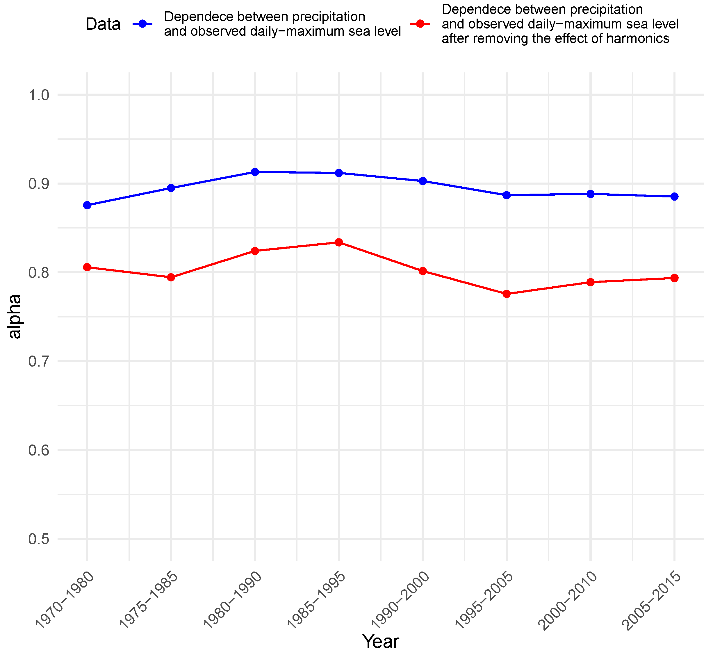
Since we have a long time series available (daily data from 1970–2016), we also assessed the temporal evolution of dependence between the precipitation and daily maximum sea level extremes with and without removing harmonics. To do this, we used the bivariate threshold excess model (outlined in Section 3.1) on a series of data subsets. Each subset represents bivariate data encompassed within a 10-year window. This moving window analysis is considered with a step size of five years. Figure 10 shows the temporal evolution of dependence, clearly showing an overall stronger dependence when we remove harmonic effects from the sea level data. The period from 1995 to 2005 shows the strongest dependence, with a value of 0.7757.

5. Discussion and Summary

This study presents the results of analyzing the dependence structure between sea level and precipitation extremes using bivariate data from Bridgeport, CT. We explored various bivariate extreme value methods, including the bivariate threshold excess model, the maxima approach, L-moments, and copulas. Our analysis shows no evidence that the occurrence of extreme values of high sea level and 24 h precipitation are correlated in the observational record at Bridgeport, CT, a station with long data records representative of coastal Connecticut. The largest surges occur in Southern New England when winds are from the east or northeast [48] due to the passage of extratropical cyclones in the colder months (November–April), or tropical cyclones in late summer. However, high precipitation rates are associated with winds from the south [49]. As both types of cyclones propagate across Southern New England, the winds from the northeast generally follow the conditions when precipitation is likely, and this may explain why the correlation is low. We further investigated the dependence structure after adjusting the effect of harmonics on the hourly sea level data to remove the periodic influences of tidal processes. These repeating patterns, while natural and significant, can obscure the underlying trends and anomalies crucial for understanding long-term sea level changes and their implications. We observed that the dependence structure between the daily maximum sea level and precipitation demonstrates a stronger dependence after adjusting for the effect of harmonics.

It is critical to note that, though the methods demonstrated here are applicable to other sites, the fact that the occurrence of extreme rain rates and coastal water levels is uncorrelated is a site-specific result. Since the character of precipitation statistics varies regionally, and tides and storm surges are sensitive to the geometry and bathymetry of the regional coastline, it seems likely that the results may apply across Southern New England. However, additional data analysis is necessary to assess that. In other parts of the world, the extremes may be much more correlated. The methods we used could also be applied to examine the relationship between extreme wave height and surge level. These may show high correlations at some sites.

The IPCC 2021 [50] concluded that it is “virtually certain” that global mean sea level will rise throughout the 21st century. They also report that for the eastern United States, there is high confidence in the predictions of an increase in the occurrence of high precipitation, and medium confidence that the wind speed during storms will also increase. However, the rate of change in extremes that we should anticipate is unclear. It is straightforward to assess the impact of a change in the mean sea level based on our results, and regional estimates of that are available. An analysis of the effect of global warming on the correlation between extreme winds and precipitation at the scales at which project information is required still needs to be conducted.

Future work could focus on investigating and applying extreme value methods to three or more variables. Extensions of the peaks-over-threshold approach [51], L-comoments [41], and the copula approach [52,53] in a multivariate framework have been developed. One could also investigate the dependence measure in a spatial framework by statistically modeling spatial extremes using max-stable processes [54], spatial copula [55], or Bayesian hierarchical models [56].

References

1. Donovan, B.; Horsburgh, K.; Ball, T.; Westbrook, G. Impacts of Climate Change on Coastal Flooding. MCCIP Sci. Rev. 2013, 2013, 211–218. [Google Scholar]
2. Kekeh, M.; Akpinar-Elci, M.; Allen, M.J. Sea Level Rise and Coastal Communities. In Extreme Weather Events and Human Health: International Case Studies; Springer: Berlin/Heidelberg, Germany, 2020; pp. 171–184. [Google Scholar]
3. Brown, S.; Nicholls, R.J.; Woodroffe, C.D.; Hanson, S.; Hinkel, J.; Kebede, A.S.; Neumann, B.; Vafeidis, A.T. Sea-Level Rise Impacts and Responses: A Global Perspective. In Coastal Hazards; Springer: Berlin/Heidelberg, Germany, 2013; pp. 117–149. [Google Scholar]
4. Jay, A.; Crimmins, A.; Avery, C.; Dahl, T.; Dodder, R.; Hamlington, B.; Lustig, A.; Marvel, K.; Méndez-Lazaro, P.; Osler, M.; et al. Ch. 1. Overview: Understanding risks, impacts, and responses. In Fifth National Climate Assessment; Crimmins, A., Avery, C., Easterling, D., Kunkel, K., Stewart, B., Maycock, T., Eds.; U.S. Global Change Research Program: Washington, DC, USA, 2023. [Google Scholar] [CrossRef]
5. Coles, S. An Introduction to Statistical Modeling of Extreme Values, 1st ed.; Springer: Berlin/Heidelberg, Germany, 2001. [Google Scholar]
6. Liu, C.; Jia, Y.; Onat, Y.; Cifuentes-Lorenzen, A.; Ilia, A.; McCardell, G.; Fake, T.; O’Donnell, J. Estimating the annual exceedance probability of water levels and wave heights from high resolution coupled wave-circulation models in long island sound. J. Mar. Sci. Eng. 2020, 8, 475. [Google Scholar] [CrossRef]
7. Pais, N.V.; Ravishanker, N.; O’Donnell, J.; Shaffer, E. Ensemble Hindcasting of Coastal Wave Heights. J. Mar. Sci. Eng. 2023, 11, 1110. [Google Scholar] [CrossRef]
8. Soukissian, T.H.; Tsalis, C. The effect of the generalized extreme value distribution parameter estimation methods in extreme wind speed prediction. Nat. Hazards 2015, 78, 1777–1809. [Google Scholar] [CrossRef]
9. Groisman, P.Y.; Karl, T.R.; Easterling, D.R.; Knight, R.W.; Jamason, P.F.; Hennessy, K.J.; Suppiah, R.; Page, C.M.; Wibig, J.; Fortuniak, K.; et al. Changes in the probability of heavy precipitation: Important indicators of climatic change. In Weather and Climate Extremes: Changes, Variations and a Perspective from the Insurance Industry; Springer: Berlin/Heidelberg, Germany, 1999; pp. 243–283. [Google Scholar]
10. Agana, N.; Sefidmazgi, M.G.; Homaifar, A. Analysis of extreme precipitation events. In Proceedings of the Fourth International Workshop on Climate Informatics, Boulder, CO, USA, 25–26 September 2014. [Google Scholar]
11. Botzen, W.; Van den Bergh, J.; Bouwer, L. Climate change and increased risk for the insurance sector: A global perspective and an assessment for the Netherlands. Nat. Hazards 2010, 52, 577–598. [Google Scholar] [CrossRef]
12. Lin-Ye, J.; Garcia-Leon, M.; Gracia, V.; Sanchez-Arcilla, A. A multivariate statistical model of extreme events: An application to the Catalan coast. Coast. Eng. 2016, 117, 138–156. [Google Scholar] [CrossRef]
13. Gudendorf, G.; Segers, J. Extreme-value Copulas. In Proceedings of the Copula Theory and Its Applications: Proceedings of the Workshop Held in Warsaw, Warsaw, Poland, 25–26 September 2009; Springer: Berlin/Heidelberg, Germany, 2010; pp. 127–145. [Google Scholar]
14. De Michele, C.; Salvadori, G.; Passoni, G.; Vezzoli, R. A multivariate model of sea storms using copulas. Coast. Eng. 2007, 54, 734–751. [Google Scholar] [CrossRef]
15. Li, F.; Zhou, J.; Liu, C. Statistical modelling of extreme storms using copulas: A comparison study. Coast. Eng. 2018, 142, 52–61. [Google Scholar] [CrossRef]
16. Li, F.; Van Gelder, P.; Ranasinghe, R.; Callaghan, D.; Jongejan, R. Probabilistic modelling of extreme storms along the Dutch coast. Coast. Eng. 2014, 86, 1–13. [Google Scholar] [CrossRef]
17. Salvadori, G.; De Michele, C. On the use of copulas in hydrology: Theory and practice. J. Hydrol. Eng. 2007, 12, 369–380. [Google Scholar] [CrossRef]
18. Renard, B.; Lang, M. Use of a Gaussian copula for multivariate extreme value analysis: Some case studies in hydrology. Adv. Water Resour. 2007, 30, 897–912. [Google Scholar] [CrossRef]
19. Favre, A.C.; El Adlouni, S.; Perreault, L.; Thiémonge, N.; Bobée, B. Multivariate hydrological frequency analysis using copulas. Water Resour. Res. 2004, 40, W01101. [Google Scholar] [CrossRef]
20. Corbella, S.; Stretch, D. Multivariate return periods of sea storms for coastal erosion risk assessment. Nat. Hazards Earth Syst. Sci. 2012, 12, 2699–2708. [Google Scholar] [CrossRef]
21. Wahl, T.; Bender, J.; Jensen, J. Copula functions as a useful tool for coastal engineers. In Proceedings of the 1st International Short Conference on Advances in Extreme Value Analysis and Application to Natural Hazards (EVAN 2013), Siegen, Germany, 18–20 September 2013; p. 56. [Google Scholar]
22. Lucey, J.T.; Gallien, T.W. Characterizing Multivariate Coastal Flooding Events in a Semi-arid Region: The Implications of Copula choice, Sampling, and Infrastructure. Nat. Hazards Earth Syst. Sci. 2022, 22, 2145–2167. [Google Scholar] [CrossRef]
23. Xu, H.; Xu, K.; Wang, T.; Xue, W. Investigating Flood risks of Rainfall and Storm Tides affected by the Parameter Estimation Coupling Bivariate Statistics and Hydrodynamic Models in the Coastal City. Int. J. Environ. Res. Public Health 2022, 19, 12592. [Google Scholar] [CrossRef]
24. Santos, V.M.; Casas-Prat, M.; Poschlod, B.; Ragno, E.; van den Hurk, B.; Hao, Z.; Kalmár, T.; Zhu, L.; Najafi, H. Multivariate Statistical Modelling of Extreme Coastal Water Levels and the Effect of Climate Variability: A case study in the Netherlands. Hydrol. Earth Syst. Sci. Discuss. 2020, 2020, 1–25. [Google Scholar]
25. Supper, H.; Irresberger, F.; Weiss, G. A Comparison of Tail Dependence Estimators. Eur. J. Oper. Res. 2020, 284, 728–742. [Google Scholar] [CrossRef]
26. Shyamalkumar, N.D.; Tao, S. On tail dependence matrices: The realization problem for parametric families. Extremes 2020, 23, 245–285. [Google Scholar] [CrossRef]
27. Gill, S.K.; Schultz, J.R. Tidal Datums and Their Applications; Oceanic and Atmospheric Administration: Silver Spring, MD, USA, 2001.
28. Menne, M.J.; Durre, I.; Vose, R.S.; Gleason, B.E.; Houston, T.G. An overview of the global historical climatology network-daily database. J. Atmos. Ocean. Technol. 2012, 29, 897–910. [Google Scholar] [CrossRef]
29. Libiseller, C.; Grimvall, A. Performance of partial Mann–Kendall tests for trend detection in the presence of covariates. Environmetrics Off. J. Int. Environmetrics Soc. 2002, 13, 71–84. [Google Scholar] [CrossRef]
30. Sen, P.K. Estimates of the regression coefficient based on Kendall’s tau. J. Am. Stat. Assoc. 1968, 63, 1379–1389. [Google Scholar] [CrossRef]
31. Hurst, H.E. Long-term storage capacity of reservoirs. Trans. Am. Soc. Civ. Eng. 1951, 116, 770–799. [Google Scholar] [CrossRef]
32. Caires, S. Extreme Value Analysis: Wave Data. JCOMM Technical Report No. 57. In Technical Report; World Meteorological Organization: Geneva, Switzerland, 2011. [Google Scholar]
33. Behrens, C.N.; Lopes, H.F.; Gamerman, D. Bayesian analysis of extreme events with threshold estimation. Stat. Model. 2004, 4, 227–244. [Google Scholar] [CrossRef]
34. Spearman, C. The proof and measurement of association between two things. In Studies in Individual Differences: The Search for Intelligence; Appleton-Century-Crofts: Colfax, NC, USA, 1961. [Google Scholar]
35. Borsos, A. Application of Bivariate Extreme Value models to describe the joint behavior of temporal and speed related surrogate measures of safety. Accid. Anal. Prev. 2021, 159, 106274. [Google Scholar] [CrossRef]
36. Beirlant, J.; Goegebeur, Y.; Segers, J.; Teugels, J.L. Statistics of Extremes: Theory and Applications; John Wiley & Sons: Hoboken, NJ, USA, 2006. [Google Scholar]
37. Sánchez-Arcilla, A.; Gomez Aguar, J.; Egozcue, J.J.; Ortego, M.; Galiatsatou, P.; Prinos, P. Extremes from scarce data: The role of Bayesian and scaling techniques in reducing uncertainty. J. Hydraul. Res. 2008, 46, 224–234. [Google Scholar] [CrossRef]
38. Goegebeur, Y.; Beirlant, J.; de Wet, T. Linking Pareto-tail kernel goodness-offit statistics with tail index at optimal threshold and second order estimation. Revstat-Stat. J. 2008, 6, 51–69. [Google Scholar]
39. Solari, S.; Losada, M. A unified statistical model for hydrological variables including the selection of threshold for the peak over threshold method. Water Resour. Res. 2012, 48, W10541. [Google Scholar] [CrossRef]
40. Asquith, W.H. Distributional Analysis with L-Moment Statistics Using the R Environment for Statistical Computing; CreateSpace: Scotts Valley, CA, USA, 2011. [Google Scholar]
41. Serfling, R.; Xiao, P. A contribution to multivariate L-moments: L-comoment matrices. J. Multivar. Anal. 2007, 98, 1765–1781. [Google Scholar] [CrossRef]
42. Sklar, M. Fonctions de répartition à n dimensions et leurs marges. In Annales de l’ISUP; HAL: Lyon, France, 1959; Volume 8, pp. 229–231. [Google Scholar]
43. Frees, E.W.; Valdez, E.A. Understanding Relationships using Copulas. N. Am. Actuar. J. 1998, 2, 1–25. [Google Scholar] [CrossRef]
44. Pugh, D.; Woodworth, P. Sea Level Science: Understanding Tides, Surges, Tsunamis and Mean Sea Level Changes; Cambridge University Press: Cambridge, UK, 2014. [Google Scholar]
45. Parker, B.B. Tidal Analysis and Prediction; Oceanic and Atmospheric Administration: Silver Spring, MD, USA, 2007.
46. Schureman, P. Manual of Harmonic Analysis and Prediction of Tides; Number 98; US Department of Commerce, Coast and Geodetic Survey: Corbin, VA, USA, 1994.
47. Codiga, D.L. Unified Tidal Analysis and Prediction Using the UTide Matlab Functions; University of Rhode Island: Narragansett, RI, USA, 2011. [Google Scholar]
48. Wong, K.C. Sea level variability in Long Island sound. Estuaries 1990, 13, 362–372. [Google Scholar] [CrossRef]
49. Agel, L.; Barlow, M.; Colby, F.; Binder, H.; Catto, J.L.; Hoell, A.; Cohen, J. Dynamical analysis of extreme precipitation in the US northeast based on large-scale meteorological patterns. Clim. Dyn. 2019, 52, 1739–1760. [Google Scholar] [CrossRef]
50. Arias, P.; Bellouin, N.; Coppola, E.; Jones, R.; Krinner, G.; Marotzke, J.; Naik, V.; Palmer, M.; Plattner, G.K.; Rogelj, J.; et al. Technical Summary. In Climate Change 2021: The Physical Science Basis. Contribution of Working Group I to the Sixth Assessment Report of the Intergovernmental Panel on Climate Change; Cambridge University Press: Cambridge, UK; New York, NY, USA, 2021; pp. 33–144. [Google Scholar] [CrossRef]
51. Rootzén, H.; Segers, J.; Wadsworth, J.L. Multivariate peaks over thresholds models. Extremes 2018, 21, 115–145. [Google Scholar] [CrossRef]
52. Griessenberger, F.; Junker, R.R.; Trutschnig, W. On a multivariate copula-based dependence measure and its estimation. Electron. J. Stat. 2022, 16, 2206–2251. [Google Scholar] [CrossRef]
53. Smith, M.S. Copula modelling of dependence in multivariate time series. Int. J. Forecast. 2015, 31, 815–833. [Google Scholar] [CrossRef]
54. Padoan, S.A.; Ribatet, M.; Sisson, S.A. Likelihood-based inference for max-stable processes. J. Am. Stat. Assoc. 2010, 105, 263–277. [Google Scholar] [CrossRef]
55. Davison, A.C.; Padoan, S.A.; Ribatet, M. Statistical modeling of spatial extremes. Statist. Sci. 2012, 27, 161–186. [Google Scholar] [CrossRef]
56. Banerjee, S.; Carlin, B.P.; Gelfand, A.E. Hierarchical Modeling and Analysis for Spatial Data; Chapman and Hall/CRC: Boca Raton, FL, USA, 2003. [Google Scholar]
Figure 1. Time series plots of the daily maximum sea level and precipitation data at Bridgeport, CT for the years 1970–2015. The color in the time series plot indicates different years.
Jmse 12 00519 g001
Figure 2. ACF plots of the precipitation, squared precipitation, daily maximum sea level, and squared daily maximum sea level data at Bridgeport, CT. The blue lines indicate values beyond which the autocorrelations are (statistically) significantly different from zero.
Jmse 12 00519 g002
Figure 3. Return level plots for daily maximum sea level and precipitation.
Jmse 12 00519 g003
Figure 4. Distribution of precipitation on days when the daily maximum sea level exceeds the 10-year return value, and the distribution of daily maximum sea level on days when precipitation exceeds the 10-year return value estimate.
Jmse 12 00519 g004
Figure 5. Scatter plot between precipitation and daily maximum sea level.
Jmse 12 00519 g005
Figure 6. CCF plot between precipitation and daily maximum sea level.
Jmse 12 00519 g006
Figure 7. Empirical joint probability distribution function plot.
Jmse 12 00519 g007
Figure 8. Return value curves for probability levels p = 0.9 , 0.95 , 0.99 using (a) the POT approach on original data, (b) the maxima approach on original data, (c) the POT approach after removing harmonic effects, and (d) the maxima approach after removing harmonic effects.
Jmse 12 00519 g008
Figure 9. Smoothed periodogram and ACF plot of the hourly sea level data.
Jmse 12 00519 g009
Figure 10. Temporal evolution of dependence from the bivariate threshold excess model between the precipitation and daily maximum sea level extremes with and without removing harmonics.
Jmse 12 00519 g010